DOI: 10.22075/JRCE.2017.11367.1186
journal homepage: http://civiljournal.semnan.ac.ir/
Hybrid Improved Dolphin Echolocation and Ant
Colony Optimization for Optimal Discrete Sizing of
Truss Structures
M. Arjmand1, M. Sheikhi Azqandi2 * and M. Delavar3 1. Department of Civil Engineering, Bozorgmehr University of Qaenat, Qaen, Iran 2. Department of Mechanical Engineering, Bozorgmehr University of Qaenat, Qaen, Iran 3. Department of Civil Engineering, Birjand University, Birjand, Iran
Corresponding author: [email protected]
ARTICLE INFO ABSTRACT
Article history:
Received: 17 May 2017 Accepted: 05 September 2017
This paper presents a robust hybrid improved dolphin echolocation and ant colony optimization algorithm (IDEACO) for optimizing the truss structures with discrete sizing variables. The dolphin echolocation (DE) is inspired by the navigation and hunting behavior of dolphins. An improved version of dolphin echolocation (IDE), as the main engine, is proposed and uses the positive attributes of ant colony optimization (ACO) to increase the efficiency of the IDE. Here, ACO is employed to improve the precision of the global optimization solution. In the proposed hybrid optimization method, the balance between exploration and exploitation process was the main factor to control the performance of the algorithm. IDEACO algorithm performance is tested on several problems of benchmarks discrete truss structure optimization. The results indicate the excellent performance of the proposed algorithm in optimum design and rate of convergence in comparison with other metaheuristic optimization methods, so IDEACO offers a good degree of competitiveness against other existing metaheuristic methods.
Keywords:
Hybrid Optimization Algorithm, Metaheuristic,
Discrete Variables, Dolphin Echolocation.
1. Introduction
The process of minimizing or maximizing an objective function is called optimization. In general, structural optimization is divided into three main types [1]. Sizing optimization, finding the area of each member of the structure. Shape (geometry) optimization, determining the coordinate nodes of the structure. Topology optimization was related to connectivity of structural
members. In most cases, the three-mentioned type optimization problem is investigated independently; however, in some problems sizing; shape and topology optimization was preformed simultaneously that is called multi modals optimization [2].
problems have studied with continuous design variables [3]. However, the accessibility of standard member sizes in the steel production sector proposes to select cross-sectional areas from an available list of discrete values. Optimization problems with discrete design variables are far more difficult to solve than problems with continuous [4].
Metaheuristic optimization methods are quite powerful and suitable for obtaining the solution to structural engineering optimization problems. The formulations of these methods are often inspired by either physical laws or natural phenomena. Meta-heuristic optimization methods consist of two phases: an exploration of the search region and exploitation of the best points found.
One of the main properties in extending an effective metaheuristic algorithm is to manage a suitable balance between exploration and exploitation [5-6].
Some of the popular meta-heuristic methods are such as genetic algorithms [7], simulated annealing optimization [8], ant colony optimization [9], particle swarm optimization [10], water cycle algorithm [11], min blast algorithm [12] and Time evolutionary optimization [13].
Each of the proposed optimization methods has specific characteristics. If the strengths and weaknesses of each method have been identified, they can be enhanced by combining two or more algorithms to reinforce the strengths and resolve the weaknesses of them. For this purpose, recently, the researchers have focused on the combination of optimization techniques. Some hybrid optimization algorithms are particle swarm optimizer, ant colony strategy and harmony search [14], charge system
search and particle swarm optimization [15], imperialist competitive and ant colony algorithm [16], water cycle and min blast algorithm [17], particle swarm optimization and convex approximation [18], colliding bodies optimization and particle swarm optimization [19], hybrid big bang crunch [20].
Dolphin echolocation is the newly meta-heuristic algorithm proposed by Kaveh and Farhoudi [21]. DE was mimicked from strategies applied by dolphins for their hunting process.
The main advantages of the dolphin echolocation algorithm are simple formulation and no essential parameter tuning. Trapping in local optima solution at the exploitation phase is one of the weaknesses of dolphin echolocation. In the present paper, for resolving this issue, at first a version of improved dolphin echolocation was proposed, and then it was combined with ant colony optimization. The efficiency of this hybrid approach is evaluated by solving a constrained classical benchmark.
2. Discrete Structural Optimization
Problems
2.1. Problem Formulation
In discrete sizing optimization of truss structures, the cost function is to minimize the total weight of the structure. The design variables are the cross-sectional area of the truss members. The optimal design must satisfy constraints such as stress and/or displacement on the structural elements and nodes, respectively.
𝑀𝑖𝑛𝑖𝑚𝑖𝑧𝑒: 𝑊(𝐴) = ∑ 𝜌𝑖 𝑁
𝑖=1
𝐴𝑖𝐿𝑖
𝑆𝑢𝑏𝑗𝑒𝑐𝑡𝑡𝑜:
{
𝜎𝑗𝑚𝑖𝑛≤ 𝜎𝑗≤ 𝜎𝑗𝑚𝑎𝑥, 𝑗 = 1,2, … , 𝑁
𝛿𝑘𝑚𝑖𝑛 ≤ 𝛿𝑘≤ 𝛿𝑘𝑚𝑎𝑥, 𝑘 = 1,2, … , 𝑀
𝐴𝑟𝜖{𝑺}, 𝑟 = 1,2, … , 𝑁
𝑺 = {𝑠1, 𝑠2, … , 𝑠𝑝}
(1)
Where W is the total weight of the structure.
𝜌𝑖, 𝐴𝑖 and 𝐿𝑖 are the structural weight, material density, cross-sectional area, and length of the ith member, respectively. N and M are the numbers of elements and nodes of truss structure respectively
𝜎𝑖is stress in ith member and 𝛿𝑖 is nodal displacement in the ith node. The superscript max and min denote the maximum and minimum limits. Each cross-sectional area must be selected from a discrete set S of p available cross-sections according to production standards.
2.2. Constraint Handling
The most common strategy in the heuristic methods to handle constrains is to apply penalty functions [25]. In this method, a constrained optimization problem was converted into an unconstrained one by multiplying a coefficient penalty by cost function based upon the value of constraint violation appears as a problem. For that reason, the pseudo cost function should be transformed into Eq. 2.
𝑊𝑝(𝐴) = [(1 + 𝜖(∑ 𝑀𝑎𝑥{0, 𝑐𝑖(𝐴)})) 𝑘
𝑖=1
2
] 𝑊(𝐴)
𝑐𝑖(𝐴) =
𝑔𝑖(𝐴)
𝑔𝑖𝑎𝑙𝑙 − 1
(2)
Where 𝑊𝑝is pseudo cost function. 𝜖 is
constant-coefficient depending on each problem. k, 𝑔𝑖(𝐴) and 𝑔𝑖𝑎𝑙𝑙 are the number of
constraints, ith constraint function consist of
stress or/and nodal displacement and allowable values of constraint, respectively.
3. Improved Dolphin Echolocation
and Ant Colony Optimization
3.1. Dolphin Echolocation Optimization
Dolphin echolocation algorithm is a new robust, and efficient Metaheuristic algorithm for solving structural optimization problems. DE is used as a simple formulation and doesn’t need extensive mathematical computations and parameter tuning. It is widely applied to various fields of optimization problems. The flowchart of the DE algorithm was illustrated in Figure 1. It can be referred to [21] for more details about this algorithm.
3.2. Ant Colony Optimization
Ant colony optimization (ACO) is a metaheuristic optimization method that was originated by Dorigo et al. [9]. The inspiring origin of this algorithm is the behavior of real ant colonies. At first, ants explore the surrounding environment of their nest randomly. On the move, ants spatter pheromone trail on the land. As soon as an ant finds a food source, it appraises the quality and the quantity of the food and carries some of them to the nest. While moving to the nest, the amount of pheromone that an ant spatters on the land can depend on the quality and quantity of the food. The pheromone instructs other ants to the food origin. It has been shown in that the indirect communication between the ants by pheromone enable them to find the shortest paths between their nest and food sources. These abilities of real ant colonies are exploited in artificial ant colonies for solving engineering problems [24]. It can be referred to [5] for more details about ACO.
3.3. Hybrid Improved Dolphin Echolocation and ant Colony Optimization
In this section, at first an improved version of the DE was proposed, and then a hybrid optimization algorithm was presented using improved dolphin echolocation and ant colony optimization. IDE optimization was introduced, which has been improved to get the best convergence and more reliable, optimal designs, especially in the final iterations and explore best results than previous studies.
IDEACO is a new hybrid improved dolphin’s echolocation and ant colony optimization algorithm. This algorithm applies to improved dolphin’s echolocation for exploration of feasible space, while
ant colony optimization is used as the exploitation of the best design.
The main steps of IDEACO for discrete optimization are summarized as follows:
Step 1. Create the alternative matrix
First, the entire search space is considered to the matrix A. The elements of this matrix consist of the value of allowable that can be assigned to design variables as follows Eq. 3.
𝐴(𝑚,𝑛𝑣𝑎𝑟)
=
[
𝐴1,1 𝐴1,2 ⋯
𝐴2,1 𝐴2,2 ⋯
⋮ ⋮ ⋱
𝐴1,𝑗 ⋯ 𝐴1,nvar
𝐴2,𝑗 ⋯ 𝐴2,nvar
⋮ ⋱ ⋮
𝐴𝑖,1 𝐴𝑖,2 ⋯
⋮ ⋮ ⋱
𝐴𝑚,1 𝐴𝑚,2 ⋯
𝐴𝑖,𝑗 ⋯ 𝐴𝑖,nvar
⋮ ⋱ ⋮
𝐴𝑚,𝑗 ⋯ 𝐴𝑚,nvar]
(3)
Where m and nvar are the number of
alternative and design variables, respectively. Elements of the matrix on each column are sorted from less to more.
Step 2. Create initial population
To start the optimization algorithm, matrix L is a candidate representing a matrix of the initial population with size (npop×nvar), which was produced randomly from matrix A as follows:
for j=1 to the number of design variables for i=1 to the number of population L(i,j) = A(randi(m), j);
end end
𝐿 =
[
𝐿1,1 𝐿1,2 ⋯
𝐿2,1 𝐿2,2 ⋯
⋮ ⋮ ⋯
𝐿1,𝑗 ⋯ 𝐿1,𝑛𝑣𝑎𝑟 𝐿2,𝑗 ⋯ 𝐿2,𝑛𝑣𝑎𝑟
⋮ ⋯ ⋮
𝐿𝑖,1 𝐿𝑖,2 ⋯
⋮ ⋮ ⋯
𝐿𝑛𝑃𝑜𝑝,1 𝐿𝑛𝑃𝑜𝑝,2 ⋯
𝐿𝑖,𝑗 ⋯ 𝐿𝑖,𝑛𝑣𝑎𝑟
⋮ ⋯ ⋮
𝐿𝑛𝑃𝑜𝑝,𝑗 ⋯ 𝐿𝑛𝑃𝑜𝑝,𝑛𝑣𝑎𝑟] (4)
Where npop is the number of population.
Step 3. Calculate the fitness of each population
hands, by decreasing the objective function (f(x)), the fitness (𝐹𝑖𝑡𝑛𝑒𝑠𝑠) must be increased. In this paper, fitness is specified as Eq. 5.
𝐹𝑖𝑡𝑛𝑒𝑠𝑠 = 𝛽
𝑓(𝑥) (5)
Where f(x) is an objective function, 𝛽 is constant-coefficient that is depended upon the type of problem that has value 10e3 in this paper.
Step 4. Sort the matrix L
The rows of matrix L based upon the fitness was sorted descending that is called SL. The fitness array of SL is SFitness as follows:
[SFitness, indF ] = sort(Fitness,1,'descend'); for j =1 to the number of design variables for i=1 to the number of population SL(i,j)=L(indF(i),j);
end end
Step 5. Calculate the effective radius
The fitness of each member’s matrix SL is distributed by radius (Ri) of them. The value of Ri depends upon the radius of the main loop (RM), number of iteration (𝐼𝑡𝑒𝑟 and
𝐼𝑡𝑒𝑟𝑚𝑎𝑥) and the place of each member on matrix SL, (𝑖) as Eq. 6. to Eq. 7.
𝑅𝑖= [𝑅𝑀− (𝑅𝑀− 1) (
𝑖 𝑛𝑃𝑜𝑝
)] , 𝑖 = 1, … , 𝑛𝑝𝑜𝑝 (6)
Where i denotes to each member of the matrix SL. RM is determined by Eq. 5.
𝑅𝑀 = [𝑅𝑚𝑎𝑥− (𝑅𝑚𝑎𝑥− 𝑅𝑚𝑖𝑛) (
𝐼𝑡𝑒𝑟 𝐼𝑡𝑒𝑟𝑚𝑎𝑥
)] (7)
Where Rmax, Rmin, Iter, and Itermax are the maximum and minimum of RM, the number of iteration in optimization procedure and the maximum number of iteration, respectively. Rmax, Rmin was selected according to the size of the search space. In this paper, the values of Rmax and Rmin are considered ¼ to ¾ of the number of alternative matrices and 2 or more than it.
Step 6. Calculate the accumulative fitness
After the calculation of Ri, the members of the matrix
SL found from matrix A and then accumulative fitness (AF) is calculated as follows (Eq. 8.):
𝐴𝐹(𝑎 + 𝑘, 𝑗) = 𝜑 (𝑅𝑖− 𝑎𝑏𝑠(𝑘) 𝑅𝑖
) 𝑆𝐹𝑖𝑡𝑛𝑒𝑠𝑠(𝑖)
+ 𝐴𝐹(𝑎 + 𝑘, 𝑗)
(8)
Where 𝜑 is calculated by Eq. 9.
𝜑 = 1
𝑖2 (9)
for i=1 to the number of population for j =1 to the number of design variables
find the place of SL(i,j) in jth column matrix A and called a
for k=-Ri to Ri
calculate AF (a+k, j) by Eq. 8. end
end end
By increasing the amount of i, the fitness of each population of the matrix SL is decreased. Parameter 𝜑increases this effect.
Accumulative fitness was distributed linearly. Figure 2 shows the distribution and their overlaps and reflects on the lower and upper bound of the design’s variables as follows:
Fig. 2. the distribution of accumulated fitness [22].
for j=1 to the number of design variables for i=1 to the number of population a=find(A(:,j)==SL(i,j));
%Calculate the radius of each member of the matrixSL Ri=Max(floor(RM-(RM-1)*i/npop),1);
for k=-Ri to Ri
if a+k<1 S=abs(a+k)+1; else if a+k>size(A,1) S=2*size(A,1)-(a+k)+1; else
end
AF(S,j)=(1/Ri)*(1/i2)*(Ri
-abs(k))*(SFitness(i))+AF(S,j); end
end end
Step 7: Obtain the best answers and create BestL matrix
The best solutions obtained, until now, is saved in BestL matrix. Matrix rows of BestL are sorted based on their fitness. The top rows of this matrix have a bigger fitness, so the first row of this matrix is the best optimal designs among the other rows. BestF is the array of the fitness of the matrix BestL.
BestL is a memory which saves some historically best design and can improve the algorithm performance, such as higher rate convergence without increasing the computational cost [23].
Step 8. Calculate the effective parameters for increasing accumulative fitness on BestL
In this step, by using the properties of ant colony optimization on continuous variables [24], the accumulative fitness of members in BestL is increased. For this purpose, parameter ω is defined as Eq. 10.
𝜔𝑖= (
1 𝑞 √2𝜋2 𝑒
−(𝑖−1)2
2𝑞2 ) , 𝑖 = 1, … , 𝑛
𝑝𝑜𝑝 (10)
Where i is each member of the population. q is defined as Eq. 11.
𝑞 = 𝐾 (1 − ( 𝐼𝑡𝑒𝑟 𝐼𝑡𝑒𝑟𝑚𝑎𝑥)
𝑃𝑜𝑤
) + 𝜀 (11)
Where K made more uniform, the amount of q and calculated by Eq. 10. Pow is dependent on the problem that has a value between 0.1 and 2. Pow and constant parameter 𝜀 are 0.4 and 1e-6, respectively.
𝐾 =
𝑓𝑖𝑡𝑛𝑒𝑠𝑠 𝑜𝑓 𝑏𝑒𝑠𝑡 𝑠𝑜𝑙𝑢𝑡𝑖𝑜𝑛 𝑖𝑛 𝑎𝑙𝑙 𝑖𝑡𝑒𝑟𝑎𝑡𝑖𝑜𝑛𝑠 𝑓𝑖𝑡𝑛𝑒𝑠𝑠 𝑜𝑓 𝑏𝑒𝑠𝑡 𝑠𝑜𝑙𝑢𝑡𝑖𝑜𝑛 𝑖𝑛 𝑐𝑢𝑟𝑟𝑒𝑛𝑡 𝑖𝑡𝑒𝑟𝑎𝑡𝑖𝑜𝑛
(12)
Step 9. Calculate the enhance probability of BestL in accumulative fitness matrix
The values of members in the accumulative fitness matrix are increased based on BestL as follows:
for j=1 to the number of population for i=1 to the number of design variables RS=Rand-selection in jth column of BestL X=find a row of RS in matrix A
Calculate AF (X, j) by Eq. 13. end
end
𝐴𝐹(𝑋, 𝑗) = (𝐴𝐹(𝑋, 𝑗) +𝐵𝑒𝑠𝑡𝐹(𝑅𝑆)
𝑅𝑆 ) 𝑁 (13)
Where N is calculated from Eq. 12.
𝑁 = 1 + 𝜔 (14)
In equations 10 to 14, by increasing coefficient i, factors 𝜔 and N will increase.
In Eq. 13, 𝐵𝑒𝑠𝑡𝐹(𝑅𝑆)
𝑅𝑆 prevents the members of
the matrix AF is zero. In addition, this term led to the algorithm can be escaped from the local minimum optimal.
Step 10. Calculate the probability of each member of matrix A
The probability of each member matrix A is calculated according to the accumulative fitness matrix by Eq. 15.
𝑃𝑖,𝑗=
𝐴𝐹𝑖,𝑗
∑ 𝐴𝐹𝑖,𝑗 𝑛𝐴𝑙𝑡 𝑖=1
, 𝑗 = 1,2, … . , 𝑛𝑣𝑎𝑟,
𝑖 = 1,2, … , 𝑛𝐴𝑙𝑡
(15)
Step 11. Rearrange the matrixL
The new matrix L is created by roulette wheel according to matrix P, as follows:
for i=1 to the number of design variables for j=1 to the number of population r=rand;
C(:,j)=(P(:,j))/(sum(P(:,j))); C(:,j)=cumsum(C(:,j)); F=find(C(:,j)>=r,1,'first'); L(i,j)=A((F),j);
Steps 3 to 11 are repeated as many times as stop criteria is satisfied.
The flowchart of IDEACO is shown in Figure3. In this flowchart, the blue step is obtained from ant colony optimization.
In main steps mentioned about IDEACO, steps 4, 7 and 9 are added, and steps 5, 6 and 10 included modified effective radius, accumulative fitness, and probability of selection, are improved compared to algorithm DE optimization.
Fig. 3. The flowchart of IDEACO algorithm.
4. Design Examples
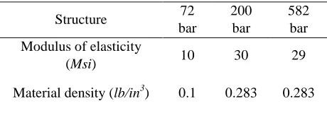
The performance of the proposed meta-heuristic algorithm was evaluated by solving three weight minimization benchmark truss structures with 72, 200, and 582 bars, including discrete variables. The material
density and modulus of elasticity of the problems are given in Table 1.
The results obtained by IDEACO are compared with those of some other popular meta-heuristic methods, presented recently in the literature. These methods are selected among various metaheuristic for evaluation considering their high computational efficiency, quality of optimal solution, and superiority of performance of the proposed method.
Table 1. Main properties of benchmark truss structures.
Structure 72
bar
200 bar
582 bar Modulus of elasticity
(Msi) 10 30 29
Material density (lb/in3) 0.1 0.283 0.283
4.1. 72-Bar Spatial Truss Structure
The layout of 72bar spatial truss structure depicted in Figure 4. This example has been investigated in [3,4,10,14,21,26]. The members of this structure are categorized in16 groups as follows:
(1) A1- A4, (2) A5- A12, (3) A13- A16, (4) A17- A18, (5) A19- A22, (6) A23- A30, (7) A31- A34, (8) A35- A36, (9) A37- A40, (10) A41- A48, (11) A49- A52, (12) A53- A54, (13) A55- A58, (14) A59- A66, (15) A67- A70, (16) A71- A72.
Two optimization cases were implemented; the discrete design variables of the cross-sectional area in both cases can be selected from the following:
Case (ii): The discrete design variables are selected from the available cross-sectional areas of the AISC code, listed in Table 2.
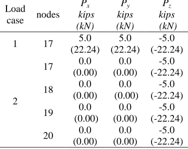
In Table 3; the loading condition of 72 bar truss structure is presented. The maximum tension or compression stress applied in members must not exceed ±25ksi (±172.38MPa). The displacement limitation of nodes is±0.25 in (6.35mm) in all coordinate directions.
The results of 72 bar truss structure are shown in Tables 4 and 5 for case (i) and case (ii) respectively.In Table 4, it can be illustrated in Case (i) the best solution is achieved using IDEACO that is better than GA, HS, and HPSO. Although it is the same as DHPACO, DE, and HHS.
Table 5 shows that in Case (ii), the results obtained using IDEACO is better than previously published works such as GA, DHPSACO, and DE.
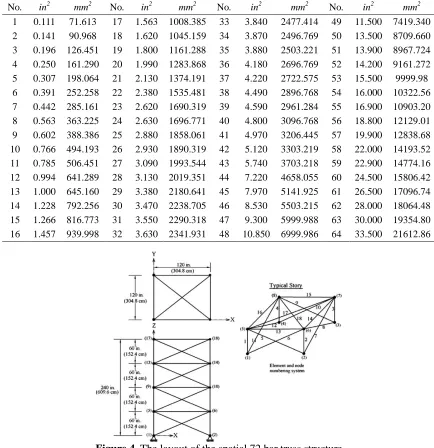
Table 2. The available cross-sectional areas for 72 bar truss structure (case (ii)). mm2 in2 No. mm2 in2 No. mm2 in2 No. mm2 in2 No. 7419.340 11.500 49 2477.414 3.840 33 1008.385 1.563 17 71.613 0.111 1 8709.660 13.500 50 2496.769 3.870 34 1045.159 1.620 18 90.968 0.141 2 8967.724 13.900 51 2503.221 3.880 35 1161.288 1.800 19 126.451 0.196 3 9161.272 14.200 52 2696.769 4.180 36 1283.868 1.990 20 161.290 0.250 4 9999.98 15.500 53 2722.575 4.220 37 1374.191 2.130 21 198.064 0.307 5 10322.56 16.000 54 2896.768 4.490 38 1535.481 2.380 22 252.258 0.391 6 10903.20 16.900 55 2961.284 4.590 39 1690.319 2.620 23 285.161 0.442 7 12129.01 18.800 56 3096.768 4.800 40 1696.771 2.630 24 363.225 0.563 8 12838.68 19.900 57 3206.445 4.970 41 1858.061 2.880 25 388.386 0.602 9 14193.52 22.000 58 3303.219 5.120 42 1890.319 2.930 26 494.193 0.766 10 14774.16 22.900 59 3703.218 5.740 43 1993.544 3.090 27 506.451 0.785 11 15806.42 24.500 60 4658.055 7.220 44 2019.351 3.130 28 641.289 0.994 12 17096.74 26.500 61 5141.925 7.970 45 2180.641 3.380 29 645.160 1.000 13 18064.48 28.000 62 5503.215 8.530 46 2238.705 3.470 30 792.256 1.228 14 19354.80 30.000 63 5999.988 9.300 47 2290.318 3.550 31 816.773 1.266 15 21612.86 33.500 64 6999.986 10.850 48 2341.931 3.630 32 939.998 1.457 16
Fig. 5. Convergence curves of the spatial 72 bar truss structure for case (i).
Fig. 6. Convergence curves of the spatial 72 bar truss structure for case (ii).
Table 3. Loading condition for 72 bar truss structure Pz
kips (kN) Py
kips (kN) Px
kips (kN)
nodes Load
case
-5.0 (-22.24) 5.0
(22.24) 5.0
(22.24) 17
1
-5.0 (-22.24) 0.0
(0.00) 0.0
(0.00) 17
2
-5.0 (-22.24) 0.0
(0.00) 0.0
(0.00) 18
-5.0 (-22.24) 0.0
(0.00) 0.0
(0.00) 19
-5.0 (-22.24) 0.0
(0.00) 0.0
(0.00) 20
Table 4. Comparison of IDEACO results with literature for the 72-bar truss structure (case (i)).
Element Group GA
[26]
HS
[4] HPSO [10]
DHPSACO [14]
DE [21]
HHS
[3] IDEACO
1 1.5 1.9 2.1 1.9 2 1.9 2
2 0.7 0.5 0.6 0.5 0.5 0.5 0.5
3 0.1 0.1 0.1 0.1 0.1 0.1 0.1
4 0.1 0.1 0.1 0.1 0.1 0.1 0.1
5 1.3 1.4 1.4 1.3 1.3 1.3 1.3
6 0.5 0.6 0.5 0.5 0.5 0.5 0.5
7 0.2 0.1 0.1 0.1 0.1 0.1 0.1
8 0.1 0.1 0.1 0.1 0.1 0.1 0.1
9 0.5 0.6 0.5 0.6 0.5 0.6 0.5
10 0.5 0.5 0.5 0.5 0.5 0.5 0.5
11 0.1 0.1 0.1 0.1 0.1 0.1 0.1
12 0.2 0.1 0.1 0.1 0.1 0.1 0.1
13 0.2 0.2 0.2 0.2 0.2 0.2 0.2
14 0.5 0.5 0.5 0.6 0.6 0.6 0.6
15 0.5 0.4 0.3 0.4 0.4 0.4 0.4
16 0.7 0.6 0.7 0.6 0.6 0.6 0.6
Best (lb) 400.66 387.94 388.94 385.54 385.54 385.54 385.54
Average (lb) 386.040 386.096
Stdev (lb) 1.155 0.6774
Table 5. Comparison of IDEACO results with literature for the 72-bar truss structure (case (ii)) Element
Group
GA [26]
DHPSACO [14]
DE
[21] IDEACO
1 0.196 1.8 2.13 1.99
2 0.602 0.442 0.442 0.563
3 0.307 0.141 0.111 0.111
4 0.766 0.111 0.111 0.111
5 0.391 1.228 1.457 1.228
6 0.391 0.563 0.563 0.442
7 0.141 0.111 0.111 0.111
8 0.111 0.111 0.111 0.111
9 1.8 0.563 0.442 0.563
10 0.602 0.563 0.563 0.563
11 0.141 0.111 0.111 0.111
12 0.307 0.25 0.111 0.111
13 1.563 0.196 0.196 0.196
14 0.766 0.563 0.563 0.563
15 0.141 0.442 0.307 0.391
16 0.111 0.563 0.563 0.563
Best (lb) 427.203 393.38 391.329 389.33
Average (lb) 390.31
Stdev (lb) 1.010
No. of analyses 10000
Figures 5 and 6 show the comparison of convergence curves for 72 bar truss structure at case (i) and case (ii) respectively.
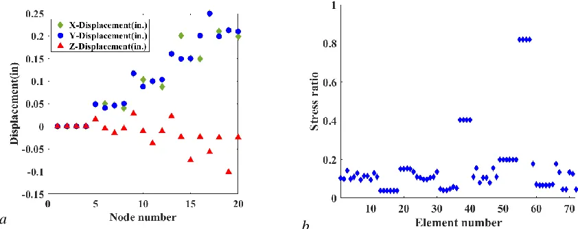
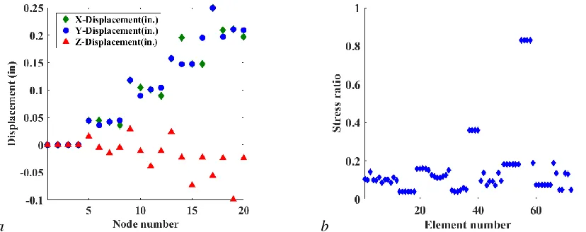
In Figures 7 and 8, the comparison of the allowable and existing constraints such as
stress ratio ( 𝜎𝑖
𝜎𝑖𝑎𝑙𝑙) for 72 bar truss structure
was shown by using IDEACO for case (i) and case (ii) respectively.
a b
a b
Fig. 8. Comparison of the allowable and existing constraints for 72 bar truss structure, case (ii): a) Displacement in all coordinate direction, b) stress ratio.
4.2. 200 Bar Planar Truss Structure
The third example considered throughout this paper is the 200-bar planar truss structure shown in Figure 9. This structure is investigated as a large-scale, size optimization problem in some recent papers [3, 27, 28, 29]. The stress limitation on members is ±10 ksi (±68.95MPa).
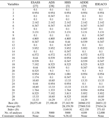
In this structure, the members are divided into 29 groups that described in Table 6. The discrete design variables of the cross-sectional area in both cases can be selected from the following:
0.1, 0.347, 0.44, 0.539, 0.954, 1.081, 1.174, 1.333, 1.488, 1.764, 2.142, 2.697, 2.8, 3.131, 3.565, 3.813, 4.805, 5.952, 6.572, 7.192, 8.525, 9.3, 10.85, 13.33, 14.29, 17.17, 19.18, 23.68, 28.08, 33.7 (in).
This structure was subjected to three loading conditions presented in Table 7.
Table 8 presents the statistical results obtained by the IDEACO algorithm and the other optimization methods.
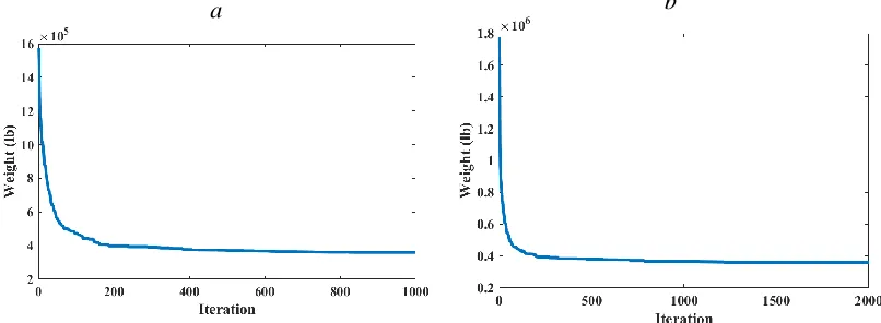
It is obvious; that IDEACO reached the superior results compared to other methods, in best, average and standard deviation which are 26831.22, 27634.24 and 371.03lb respectively, in over 12000 numbers of analyses. Figure10 depicts the convergence curves of 200 bar truss structure.
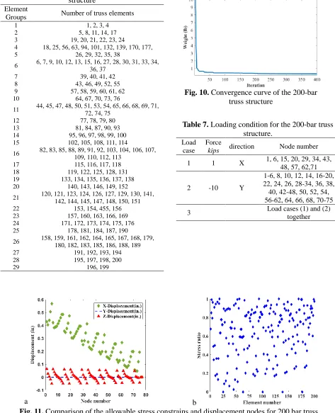
In Figure11, for 200 bar truss structure, the comparison of the allowable stress constraints for elements and displacement of nodes were shown by using IDEACO.
Table 6. The design variables in the 200 bar truss structure
Number of truss elements Element
Groups
1, 2, 3, 4 1
5, 8, 11, 14, 17 2
19, 20, 21, 22, 23, 24 3
18, 25, 56, 63, 94, 101, 132, 139, 170, 177, 4
26, 29, 32, 35, 38 5
6, 7, 9, 10, 12, 13, 15, 16, 27, 28, 30, 31, 33, 34, 36, 37
6
39, 40, 41, 42 7
43, 46, 49, 52, 55 8
57, 58, 59, 60, 61, 62 9
64, 67, 70, 73, 76 10
44, 45, 47, 48, 50, 51, 53, 54, 65, 66, 68, 69, 71, 72, 74, 75
11
77, 78, 79, 80 12
81, 84, 87, 90, 93 13
95, 96, 97, 98, 99, 100 14
102, 105, 108, 111, 114 15
82, 83, 85, 88, 89, 91, 92, 103, 104, 106, 107, 109, 110, 112, 113
16
115, 116, 117, 118 17
119, 122, 125, 128, 131 18
133, 134, 135, 136, 137, 138 19
140, 143, 146, 149, 152 20
120, 121, 123, 124, 126, 127, 129, 130, 141, 142, 144, 145, 147, 148, 150, 151 21
153, 154, 455, 156 22
157, 160, 163, 166, 169 23
171, 172, 173, 174, 175, 176 24
178, 181, 184, 187, 190 25
158, 159, 161, 162, 164, 165, 167, 168, 179, 180, 182, 183, 185, 186, 188, 189 26
191, 192, 193, 194 27
195, 197, 198, 200 28
196, 199 29
Fig. 10. Convergence curve of the 200-bar truss structure
Table 7. Loading condition for the 200-bar truss structure.
Node number direction
Force
kips
Load case
1, 6, 15, 20, 29, 34, 43, 48, 57, 62,71 X
1 1
1-6, 8, 10, 12, 14, 16-20, 22, 24, 26, 28-34, 36, 38, 40, 42-48, 50, 52, 54, 56-62, 64, 66, 68, 70-75 Y
-10 2
Load cases (1) and (2) together 3
a b
Table 8. Comparison of IDEACO results with literature for the 200-bar truss structure
Variables ESASS
[27]
ADS [28]
HHS [3]
ADDE
[29] IDEACO
1 0.1 0.1 0.1 0.1 0.1
2 0.954 0.954 0.954 0.954 0.954
3 0.1 0.347 0.1 0.1 0.1
4 0.1 0.1 0.1 0.1 0.1
5 2.142 2.142 2.142 2.142 2.142
6 0.347 0.347 0.347 0.347 0.347
7 0.1 0.1 0.1 0.347 0.1
8 3.131 3.131 3.131 3.131 3.131
9 0.1 0.1 0.1 0.1 0.347
10 4.805 4.805 4.805 4.805 4.805
11 0.347 0.44 0.44 0.539 0.347
12 0.1 0.1 0.347 0.1 0.1
13 5.952 5.952 5.952 5.952 5.952
14 0.1 0.1 0.347 0.1 0.1
15 6.572 6.572 6.572 6.572 6.572
16 0.44 0.539 0.954 0.440 0.539
17 0.539 0.1 0.347 0.539 0.347
18 7.192 8.525 8.525 8.525 8.525
19 0.44 0.539 0.1 0.347 0.44
20 8.525 9.3 9.3 9.3 9.3
21 0.954 0.954 1.081 0.954 0.954
22 1.174 0.1 0.347 0.1 0.1
23 10.85 10.85 13.33 13.33 13.33
24 0.44 0.954 0.954 0.1 0.1
25 10.85 13.33 13.33 13.33 13.33
26 1.764 1.333 1.764 0.954 0.954
27 8.525 7.192 3.813 5.952 5.952
28 13.33 10.85 8.525 10.85 10.85
29 13.33 14.29 17.17 14.29 14.29
Best (lb) 28,075.49 27,190.49 27,163.59 26960.152 26831.22
Average (lb) 28,159.59 27969.510 27634.24
Stdev (lb) 1149.91 422.130 371.03
No. of analyses 11,156 5000 5000 6189 12,000
Constraint violation None None %36.42 None None
4.3. 582 Bar Planar Truss Structure
In Figure 12, the layout of 582bar spatial truss structure was presented. In this structure, the members are divided into 32 groups, as showed in Figure 12. This example has been investigated in [14, 21, 30, 31].
The discrete design variables of the cross-sectional area can be selected from 140 economic standard steel W-shape profile list based on the area and radius of gyration properties. The lower and upper bounds on cross-sectional areas of all elements can be
taken as between 39.74 and 1378.09 cm2 (6.16 and 215 in2).
This tower structure was subject to a single load case, the lateral loads of 5 kN (1.12 kips) and 30 kN (6.74 kips) applied in both x and y directions and in the z-direction at all nodes, respectively. The nodal displacement of nodes must not exceed 3.15 in (80 mm).The stress limitations of the members are considering, according to ASD-AISC as Eq. 16.
{𝜎𝑖
𝑇= 0.6𝐹 𝑦𝜎𝑖> 0
𝜎𝑖𝐶𝜎𝑖< 0
Where𝜎𝑖𝐶can be computed according to the slenderness ratio as Eqs. 17 and 18.
Fig. 12. The layout of the 582-bar spatial truss structure.
𝜎𝑖𝐶=
{ (1−𝜆𝑖2
2𝐶𝑖2) 𝐹𝑦
(5 3+
3𝜆𝑖 8𝐶𝑐−
𝜆𝑖3 8𝐶𝑐3)
𝜆𝑖< 𝐶𝑐
12𝜋2𝐸
23𝜆2𝑖
𝜆𝑖≥ 𝐶𝑐
(17)
𝐶𝑐 = √
2𝜋2𝐸
𝐹𝑦
(18)
Where E, 𝜆and 𝐹𝑦are the modulus of
elasticity, the slenderness ratio (λi = kiLi⁄ri)
and the yield stress (248 MPa (36ksi)) according to ASD-AISD respectively. The slenderness ratio divides the elastic and inelastic buckling regions by Cc.Li is the slenderness ratio, ri, and kiare radius of gyration and effective length factor, respectively.
The slenderness ratio must not exceed 300 and 200 for tension and compression members, respectively. If for compression members, the slenderness ratio was more than 200, the value of stress in these members should be less than the value
calculated by12𝜋
2𝐸
23𝜆𝑖2 .
This tower structure is analyzed for two different cases as follows.
case (i): maximum number of iteration in the optimization process is considered 1000.
case (ii): maximum number of iteration in the optimization process is considered 2000.
The optimization results of 582 bar truss structure are shown in Table 9. The results obtained by IDEACO are the superiors compared with other methods, in best, average, worst, standard deviation, and number of analysis in both cases.
a b
a b
Fig. 14. Comparison of the allowable stress constrains and displacement nodes for 582 bar truss structure, a) Displacement in all coordinate direction, b) stress ratio.
Table9. Comparison of IDEACO results with literature for the 582-bar truss structure.
Case (i) Case (ii)
Variables PSO
[30]
ABC [31]
DHPSACO [14]
DE
[21] IDEACO
ABC [31]
DE
[21] IDEACO
1 W8×21 W8×22 W8×24 W8×21 W8×21 W8×22 W8×21 W8×21
2 W12×79 W12×97 W12×72 W12×96 W14×90 W10×78 W27×94 W14×90
3 W8×24 W8×25 W8×28 W8×24 W8×024 W8×25 W8×24 W8×24
4 W10×60 W12×59 W12×58 W12×58 W10×60 W14×62 W12×58 W14×61
5 W8×24 W8×24 W8×24 W8×24 W8×24 W8×24 W8×24 W8×24
6 W8×21 W8×21 W8×24 W8×21 W8×21 W8×21 W8×21 W8×21
7 W14×48 W12×46 W10×49 W12×45 W10×49 W12×51 W12×50 W14×48
8 W8×24 W8×24 W8×24 W8×24 W8×24 W8×24 W8×24 W8×24
9 W8×21 W8×21 W8×24 W8×21 W8×21 W8×21 W8×21 W8×21
10 W10×45 W12×46 W12×40 W12×45 W14×43 W10×50 W12×45 W10×45
11 W8×24 W8×22 W12×30 W8×21 W8×21 W8×25 W8×21 W8×21
12 W10×68 W12×66 W12×72 W12×65 W16×67 W10×69 W12×72 W16×67
13 W14×74 W10×77 W18×76 W10×77 W18×76 W18×77 W14×74 W14×74
14 W14×48 W10×49 W10×49 W10×49 W10×45 W14×49 W12×50 W10×45
15 W18×76 W14×83 W14×82 W14×82 W14×74 W10×78 W10×68 W18×76
16 W8×31 W8×32 W8×31 W8×31 W8×31 W8×32 W8×31 W8×31
17 W16×67 W12×53 W14×61 W10×60 W16×67 W21×62 W14×61 W16×67
18 W8×24 W8×24 W8×24 W8×24 W10×22 W8×24 W8×24 W10×22
19 W8×21 W8×21 W8×21 W8×21 W8×21 W8×21 W8×21 W8×21
20 W8×40 W16×36 W12×40 W12×45 W14×43 W14×43 W14×43 W14×43
21 W8×24 W8×24 W8×24 W8×21 W8×21 W8×24 W8×21 W8×21
22 W8×21 W10×22 W14×22 W8×21 W8×21 W8×21 W8×21 W8×21
23 W10×22 W10×22 W8×31 W10×22 W8×24 W8×24 W6×25 W8×24
24 W8×24 W6×25 W8×28 W8×21 W8×21 W8×24 W8×21 W8×21
25 W8×21 W8×21 W8×21 W8×21 W8×21 W8×21 W8×21 W8×21
26 W8×21 W8×21 W8×21 W8×21 W8×21 W8×21 W8×21 W8×21
27 W8×24 W8×24 W8×24 W8×21 W8×21 W8×24 W8×21 W8×21
28 W8×21 W8×21 W8×28 W8×21 W8×21 W8×21 W8×21 W8×21
29 W8×24 W8×22 W16×36 W8×21 W8×21 W8×21 W8×21 W8×21
30 W8×21 W10×23 W8×24 W8×21 W8×21 W8×21 W8×21 W8×21
31 W8×21 W8×25 W8×21 W8×21 W8×21 W8×24 W8×21 W8×21
32 W8×24 W6×26 W8×24 W8×21 W8×21 W8×24 W8×21 W8×21
Best (lb) 363795.7 368484.1 380982.7 360367.8 357933.4 365906.3 360143.3 357906.6
Average (lb) 365124.9 370178.6 364404.7 359357.6 366088.4 362207.1 358830.8
Worst (lb) 370159.1 373530.3 371922.1 361499.0 369162.2 367512.2 360534.2
Stdev (lb) 1176.40 1133.24
No. of
In case (i), the best design in IDEACO algorithm was 1.64%, 2.95%, 6.44%, and 0.68% lighter than PSO, ABC, DHPSACO, and DE respectively. In case (ii), the best design in IDEACO algorithm was 2.24% and 0.63% lighter than ABC and DE respectively.
Figure 13 depicts the convergence curve of 582 bar spatial truss structure in both cases.
In Figure 14, for 582 bar truss structure, the comparison of the allowable stress constraints for elements and displacement of nodes was shown by using IDEACO.
5. Conclusion
In this paper, a new hybrid optimization algorithm was presented, including dolphin echolocation and ant colony optimization. This algorithm can be applied for discrete sizing optimization problems such as truss structures. At first, the DE was improved as called IDE, and then it is hybridized with ant colony optimization algorithm to use solution benchmark structural optimization problems. The performance and efficiency of IDEACO were tested extensively using four benchmark truss structure optimization problems. The comparison of the numerical result received by IDEACO and other optimization methods are presented. These results verify the efficiency, effectiveness, and robustness of the proposed method.
The IDEACO algorithm yielded better results than optimization methods applied for comparison in convergence capability and optimum design. Almost in all design problems, the proposed algorithm reached a result that is better than or similar to literature and needed much fewer structural analyses. So, hybridization of the IDE and ACO not only may lead to a balance between exploitation and exploration but also improve
convergences to optimum design. IDEACO is the desired method for solving complex problems, and the hybrid method is surely an issue to be studied in future researches.
REFERENCES
[1] Hare, W., Nutini, J., Tesfamariam, S. (2013). “A survey of non-gradient optimization methods in structural engineering.” Advances in Engineering Software, Vol. 59, pp. 19–28.
[2] Leandro Fleck Fadel Miguel, L. F. F., Rafael Holdorf Lopez, R. H., Miguel, L. F. F. (2013). “Multimodal size, shape, and topology optimisation of truss structures using the Firefly algorithm.” Advances in Engineering Software, Vol. 56, pp. 23–37. [3] Min-Yuan Cheng, M. Y., Prayogo, D. Yu-Wei W., Lukito, M. M., (2016). “A Hybrid Harmony Search algorithm for discrete sizing optimization of truss structure.” Automation in Construction, Vol. 69, pp. 21–33.
[4] Lee, K. S., Geem, Z. W., Lee, S. H., Bae, K. W., (2005). “The harmony search heuristic algorithm for discrete structural optimization.” Engineering Optimization, Vol. 37, Issue 7, pp. 663–684.
[5] Ghoddosian, A., Sheikhi, M., (2013). “Metaheuristic optimization methods in engineering.” Semnan University Press. [6] Kaveh, A., Mahdavi, V. R., (2015). “A hybrid
CBO–PSO algorithm for optimal design of truss structures with dynamic constraints.” Applied Soft Computing, Vol. 34, pp. 260– 273.
[7] Rajeev, S., Krishnamoorthy, C. S. (1992). “Discrete optimization of structures using genetic algorithms.” Journal of Structural Engineering, Vol. 118, Issue 5, pp. 1233-1250.
Methods in Engineering, Vol. 38, Issue 16, pp. 2753-2773.
[9] Camp, C. V., Bichon, B. J., (2004). “Design of space trusses using ant colony optimization.” Engineering Optimization, Vol. 130, Issue 5, pp. 741-751.
[10] Li, L. J., Huang, Z. B., Liu, F., (2009). “A heuristic particle swarm optimization method for truss structures with discrete variables.” Computer Structures., Vol. 87, Issue 7, pp. 435-443.
[11] Eskandar, H., Sadollah, A., Bahreininejad, A., Hamdi, M., (2012). “Water cycle algorithm – A novel metaheuristic optimization method for solving constrained engineering optimization problems.” Computers Structures, Vol. 110, pp. 151–166.
[12] Sadollah, A., Bahreininejad, A., Eskandar, H., Hamdi, M., (2012). “Mine blast algorithm for optimization of truss structures with discrete variables.” Computers Structures, Vol. 102, pp. 49– 63.
[13] Sheikhi, M., Delavar, M., Arjmand, M., (2016). “Time evolutionary optimization: A new meta-heuristic optimization algorithm.” Proceedings of the 4th International Congress on Civil Engineering, Architecture and Urban Development, Shahid Beheshti University, Tehran, Iran.
[14] Kaveh, A., Talatahari, S., (2009). “Particle swarm optimizer, ant colony strategy and harmony search scheme hybridized for optimization of truss structures.” Computer Structures, Vol. 87, pp. 267-283.
[15] Kaveh, A., Talatahari, S., (2012). “A hybrid CSS and PSO algorithm for optimal design of structures.” Structural Engineering and Mechanics, Vol. 42, Issue 6, pp.783-797. [16] Sheikhi, M., Ghoddosian, A., (2013). “A
hybrid imperialist competitive ant colony algorithm for optimum geometry design of frame structures, Structural Engineering and Mechanics.” Vol. 46, Issue 3, pp. 403-416.
[17] Sadollah, A., Eskandar, H., Bahreininejad, A., Kim, J. H., (2015). “Water cycle, mine
blast and improved mine blast algorithms for discrete sizing optimization of truss structures.” Computers Structures, Vol. 149, pp. 1–16.
[18] Shojaee, S., Arjomand, M., Khatibinia, M., (2013). “A hybrid algorithm for sizing and layout optimization of truss structures combining discrete PSO and convex approximation,” International Journal ofOptimization in Civil Engineering, Vol 3, Issue 1, pp. 57-83.
[19] Kaveh, A., Mahdavi, V. R., (2015). “A hybrid CBO–PSO algorithm for optimal design of truss structures with dynamic constraints.” Applied Soft Computing, Vol. 34, pp. 260–273.
[20] Lotfi, H., Ghoddosian, A., (2015). “Size and Shape Optimization of Two-Dimensional Trusses Using Hybrid Big Bang-Big Crunch Algorithm.” International journal of mechatronics, electrical and computer technology, Vol. 5, Issue 14, PP. 1987-1998.
[21] Kaveh, A., Farhoudi, N., (2013). “A new optimization method: Dolphin echolocation.” Advances in Engineering Software, Vol. 59, pp. 53–70.
[22] Kaveh, A., Hosseini, P., (2014). “A simplified dolphin echolocation optimization method for optimum design of trusses.” International Journal of Optimization in Civil Engineering, Vol. 4, Issue 3, pp. 381-397.
[23] Kaveh, A., IlchiGhazaan, M., (2014). “Enhanced colliding bodies optimization for design problems with continuous and discrete.”Advances in Engineering Software, Vol. 77, pp. 66–75.
[24] Socha, K., Blum, Ch., (2007). “An ant colony optimization algorithm for continuous optimization: application to feed-forward neural network training.” Neural Computing and Applications, Vol. 16, pp. 235-247.
Methods in Applied Mechanics and Engineering, Vol.191, pp. 1245–1287. [26] Wu, S. J, Chow, P. T. (1995). “Steady-state
genetic algorithms for discrete optimization of trusses.” Computer Structure, Vol. 56, pp. 979–91.
[27] Azad, S. K., Hasançebi, O., (2014). “An elitist self-adaptive step-size search for structural design optimization.” Applied Soft Computing, Vol. 19, pp. 226-235. [28] Azad, S. K., Hasançebi, O., (2015).
“Discrete sizing optimization of steel trusses under multiple displacement constraints and load cases using guided stochastic search technique.” Structural and Multidisciplinary Optimization, Vol. 52, Issue 2, pp. 383-404.
[29] Pham, A. H., (2016). “Discrete optimal sizing of truss using adaptive directional differential evolution.” Advances in Computational Design, Vol. 1, Issue 3, pp. 275-296.
[30] Hasancebi, O., Carbas, S., Dogan, E., Erdal F., Saka M. P. (2009). “Performance evaluation of metaheuristic search techniques in the optimum design of real size pin jointed structures.” Computer Structures, Vol. 87, Issue 5, pp.284–302. [31] Sonmez, M., (2011). “Discrete optimum
![Fig. 1. The flowchart of dolphin echolocation [21].](https://thumb-us.123doks.com/thumbv2/123dok_us/8957776.1867144/3.612.315.522.364.645/fig-flowchart-dolphin-echolocation.webp)
![Fig. 2. the distribution of accumulated fitness [22].](https://thumb-us.123doks.com/thumbv2/123dok_us/8957776.1867144/5.612.330.528.448.578/fig-distribution-accumulated-fitness.webp)