* Corresponding author Tel: +989125909976. E-mail address: [email protected] (M. M. Tahernejad).
Journal Homepage: ijmge.ut.ac.ir
Analyzing the effect of ore grade uncertainty in open pit mine planning; a
case study of the Rezvan iron mine, Iran
Mohammad Mehdi Tahernejad
a, *, Reza Khalokakaie
a, Mohammad Ataei
aaFaculty of Mining, Petroleum and Geophysics Engineering, Shahrood University of Technology, Shahrood, Iran
ABSTRACT
Due to uncertain nature of grade in ore deposits, considering uncertainty is inevitable in geological modeling of resources and mine planning. In other words, uncertainty in grade of mineralized materials is one of the most significant parameters that need attention in mine planning. In this paper, a comparative procedure utilizing Sequential Gaussian Simulation (SGS) and traditional Ordinary Kriging (OK) was applied in an iron ore mine, and the influence of ore grade uncertainty in mine planning was investigated. It was observed that the grade distribution resulted from the SGS is almost identical to that of the real exploration data as compared to the OK method. In addition, uncertainties including ore grade of deposit would significantly affect the technical and financial aspects of the plans. The comparison shows that the simulation-based ultimate pits exhibit less risk in deviating from quantity and quality targets than the traditional approaches based on a single orebody model obtained by the OK method. Using the SGS method, there was an increase in the value of the net present value of mine plans. Keywords : Grade estimation, Mine planning, Ordinary Kriging, Sequential Gaussian simulation, Ore grade uncertainty
1.
Introduction
Open pit mining is an extractive activity prepared for the purpose of exploitation of economically valuable minerals or materials from the earth as the largest source of metals and minerals. Ultimate pit limit determination is the most important part of mine planning that defines the limits of the ore deposit up to which it is economically feasible to mine [1]. It establishes the tonnages of mineable reserves, ore and waste and the location of other surface facilities such as ore stockpiles and waste dumps [2]. Open pit mine planning is determining the parts of a deposit to be mined annually to maximize the total net present value (NPV) of the mining project [1]. Optimizing the production scheduling is a process that deals with the management of cash flows in the order of hundreds of millions of dollars and is heavily impacted by uncertainty in the ore and waste forecasted to be produced from a pit in both valuations and operation [3]. Uncertainty about the spatial distribution of ore grade can cause deviations from production targets [4, 5]. This is largely due to the propagation of errors in understanding the orebodies throughout the chain of mining [6].
In traditional approaches, an orebody model containing the deposit features such as ore grades was used for mine planning. The main drawback of estimation techniques is that they are unable to reproduce the in-situ variability of the deposit grades as inferred from the available data [6]. The Uncertainty that caused by the single estimated value of a block cannot represent the possible in situ grade variations between the sampled points [1]. Geostatistical estimation methods, such as Kriging, have long been used to model the spatial distribution of grades of interest within the mining blocks representing a deposit. In the conventional Kriging grade modeling, undesirable underestimating and/or overestimating due to smoothing effect may occur. Ordinary Kriging, one of the most reliable local estimation methods, correspondingly suffers from the smoothing effect because of simply the averaging nature of the Kriging algorithm. Kriging estimates do not
reproduce the sample histogram because of reduced variance of the smoothing effect. In the OK estimation process, low values are overestimated and high values are underestimated [7]. To overcome the drawbacks of the conventional method and especially to consider the uncertainty during an ore grade estimation, some methods such as the conditional simulation may be useful. The conditional simulation technique uses geostatistical parameters to construct the number of grade distribution realizations with equal probability [8].
The significance of the ore grade uncertainty in open-pit mining has received significant attention in recent years and it is well acknowledged in the literature. Initially, Ravenscroft [9] discussed the risk analysis in mine planning based on the orebody realizations. In addition, conditional simulation is used to integrate the grade uncertainty in various related aspects of open pit mining such as mine planning [10, 11]. Dimitrakopoulos and Ramazan [12] suggested a methodology that was based on the probabilities of ore grades being above the cutoffs. To calculate the mentioned probabilities, they used a simulation method to make realizations of the orebody. Godoy and Dimitrakopoulos [13] generated the production schedules for all realizations of the orebody and then combined the mining sequences in order to produce a single schedule. Ramazan and Dimitrakopoulos [14] as well as Menabde and Froyland [15] used the simulated orebodies to calculate the extraction probability of each block in a given period. Dimitrakopoulos et al. [16] applied the conditional simulation and showed a remarkable deviation from the project targets that may cause in planning with a single ore body model. Dimitrakopoulos et al. [17] proposed a new approach in which different deposit simulations were compared, and the best one was selected. They used conditional simulations to obtain the candidate plans based on several orebody models. Ramazan and Dimitrakopoulos [18] engaged the integrated conditional simulation and stochastic integer programming for the NPV maximization. Furthermore, Whittle and Bozorgebrahimi [19] used the conditional simulations to generate the so-called Hybrid Pits. Godoy and Dimitrakopoulos [20] presented a set of procedures that would enable mine-planning engineers to carry
out a series of analyses, which could be used to evaluate the sensitivity of pit designs to the grade uncertainty. Dimitrakopoulos [6] proposed a new mine planning paradigm employing the sequential simulation approach to simulate pertinent attributes of mineral deposits. An extended mathematical framework was provided that allowed direct integration of orebody uncertainty to mine design, production planning, and valuation of mining projects and operations. Goodfellow and Dimitrakopoulos [21] used geological simulations with the simulated annealing algorithm to modify an initial design to minimize the variability of the material that is sent to each destination. Gholamnejad and Moosavi [22] incorporates the geological uncertainty within the orebody that was developed with a new binary integer-programming model for long-term production scheduling. Ramazan and Dimitrakopoulos [1] developed and applied a new stochastic integer-programming model to a gold deposit in Australia. They used multiple conditionally simulated orebody models for optimizing the annual production schedules in open pit mines. Other studies in the literature are regarding the application of conditional simulation [4, 23-25].
In this paper, in order to demonstrate the impact of the ore grade uncertainty and the relative effects on planning results in iron ore mines, a case study of the Rezvan iron ore mine was provided in the paper. Therefore, a geological block model was constructed for the Rezvan iron ore mine and was implemented in the geostatistical analysis. Thereafter, considering economic block model, the open pit parameters including average grade, mineable ore, waste tonnage, and net present value (NPV) were determined for both SGS and OK methods. In this way, this paper quantified the ore grade uncertainty in ultimate pit determination and mine planning. Moreover, the advantages of utilizing SGS method over the conventional OK method in grade estimation and mine planning in uncertain condition were investigated in iron ore mines.
2.
SGS background
A set of equally probable models of the deposit can be used as an input for an optimization mine design. The models present the actual and unknown spatial distribution of grades [6]. SGS is a variogram-based simulation procedure and a special case that takes advantage of convenient properties of Gaussian random functions [26]. SGS is a widely used algorithm for modeling reservoir properties. Conditional simulations of orebodies utilizing SGS method are identified as a standard tool to model this kind of uncertainty [4, 5, 10, 24]. Unlike the Kriging method, conditional simulation generates the grade models that do not suffer from the smoothing effect, and therefore, can be utilized for investigating the intrinsic uncertainty related to the estimated ore grades. The SGS algorithm uses the sequential simulation formalism to simulate a Gaussian random function. Let Y(u) be a multivariate Gaussian random function with a zero mean value, unit variance, and a given variogram model γ(h). Realizations of Y(u) can be generated by the following algorithm [26]:
1. Define a random path visiting each node of the grid 2. for each node u along the path do
3. Get the conditioning data consisting of neighboring original hard data (n) and previously simulated values
4. Estimate the local conditional cumulative distribution function (ccdf) as a Gaussian distribution with mean given by kriging and variance by the kriging variance
5. Draw a value from that Gaussian ccdf and add the simulated value to the dataset
6. end for
7. Repeat for another realization
3.
Case study
The Rezvan iron ore deposit located in a mountainous region is situated 75 km north of Bandar Abbas, in the Hormozgan Province of Iran, between 56°07′E longitude and 27°40′N latitude with an average altitude of 1,000 m above the sea level. This region has a dry climate with
moderate to warm temperature. In this paper, part of the deposit that has sufficient exploration data was considered as the study area.
3.1.Data preparation
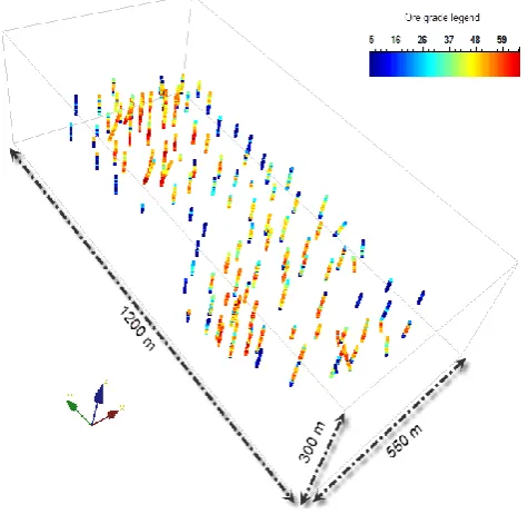
The data used in geostatistical modeling were obtained from 125 vertical exploration boreholes with azimuths of 0–355° and dips of 70– 90° drilled over the mining area shown in Fig. 1. The holes were drilled in a semi-regular pattern in a 550 meters (E–W) by 1200 meters (N–S) area with about 50 meters spacing between the adjacent drill holes. The information includes 3483 powder samples. The total length of the drill holes is 6966 meters.
Fig. 1. Spatial locations of boreholes samples (“x” and “y” directions indicate Easting and Northing respectively).
3.2.Statistical analysis of input data
In order to start the geostatistical analysis, it is necessary to perform a preliminary statistical analysis including compositing, recognizing the outlier data, finding out the trends, and if necessary, conversion of abnormal to normal distributions. The Dorfel test was performed to distinguish the outlier data, which showed no outliers in the input data. Moreover, no specific trend for the grade was distinguished. Before calculating the variogram, it needs to examine both the spatial distribution of sampling sites and the cumulative distribution of the measurements to assess any need to modify the original data [28]. Based on Fig. 1, it seems that the boreholes are not located on a regular grid. To avoid the effects of preferential sampling and further biased results of the predictive models, the data were de-clustered and the output file used to transform the data into a normal distribution, for input to variogram analysis, OK and SGS process. The frequency distribution of grade of samples was checked for evaluation of Gaussian behavior. Fig. 2 shows the histogram of samples grade and statistical parameters of the distributions are given in Table 1. Fig. 2 showed that the data did not exactly possess a Gaussian distribution. Therefore, the ore grade distribution in this work was transformed into normal scores by targeting a Gaussian distribution with mean 0 and variance 1. However, the values of the attributes were transformed back to the original space during the simulations by targeting the original distribution.
3.3.Spatial correlation analyses using variograms
spatial correlation analyses. SGeMS implements several geostatistics algorithms for modeling of the phenomenon that exhibit the space distributions [26]. Variogram analysis, which allows for examination of whether the data are correlated with distance, was applied on the ore grade. If a spatial correlation emerges in the dataset, directional variograms should start from low values and increase up to the variance of the sample data. The knowledge of spatial correlations and ranges over which such correlations are observed, along with the knowledge of the mean of the data, are also taken into consideration when estimating the spatial distribution of parameters and their uncertainty [29]. The semivariogram, γ(h), measures the average dissimilarity between two regionalized variable; for example between the values of a parameter (x) at location u and location u+h. Assuming stationarity, the semivariogram γ(Z(u), Z(u+h)) depends on a lag vector h: γ(h). Thus, the experimental semivariogram is computed by [26]:
h N
2
h u Z u Z h 2N
1 h γ
(1)
Fig. 2. Ore grade frequency distribution and the probability of samples data.
Table 1. Statistical parameters of the samples data.
No. of samples
Average grade (%)
Std (%)
Min (%)
Max (%)
Kurtosis Skewness
3483 44.97 10.31 15.01 64.98 0.32 -0.88
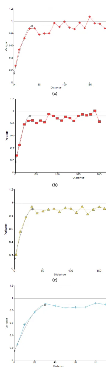
In this equation, z(u) is the value of the parameter at location u and N(h) is the number of data pairs separated by vector h. Trying various lag distance base on borehole collar spacing, it was found that a lag of 30 meters gives the best fit for spherical model applicable. Fig. 3 illustrates four selected directional experimental variograms of normal scores of samples data. Observing the obtained variograms, an anisotropy was detected. Specifications of the spherical models are given in Table 2.
In this section, the cross-validation method was used to evaluate the validation of the fitted variogram models. Fig. 4 represents the correlation plot of actual and estimated values in the cross-validation test. An acceptable match between the actual and estimated values with the correlation coefficient equal to 0.84 can be seen from this plot. Fig. 5 shows the frequency distribution plot for the difference of actual and estimated values. It can be seen from the plot that the difference of actual and estimated values have almost normal distribution with a mean value equal to -0.173. It can be conclude from this plots that the variogram models are sufficiently valid in the estimation and simulation processes. The selected parameters for Kriging is mentioned in Table 3.
(a)
(b)
(c)
(d)
Fig. 3. Directional variograms of normal scores of samples data ((a), (b) and (c) illustrate the horizontal direction at azimuth 0°, 45° and 90° respectively, and (d)
Table 2. Specifications of the spherical models fitted on directional variograms. Model Nugget
(%2) (%Sill 2) Azimuth (degree) (degree) Dip Rang (m)
Spherical 0.15 0.75 0 0 38
45 0 35
90 0 33
135 0 35
- 90 30
Fig. 4. Correlation plot of actual and estimated values in the cross-validation test.
Fig. 5. Frequency distribution chart for the difference of actual and estimated values in the cross-validation test.
Table 3. Optimum parameters for ordinary kriging.
Range-1 (m)
Range-2 (m)
Range-3 (m)
Minimum number of points used for
estimation
Maximum number of points used for
estimation
38 33 30 48 5
3.4.Geostatistical modeling and simulation
3.4.1.Kriging implementation
Kriging is a group of geostatistical techniques to interpolate the value of a random field at an unobserved location from the observations of its value at nearby locations. In Kriging, an estimated grade of a block within an orebody model generates a weighted average of the surrounded samples while the actual grade is unknown. Depending on the mean value specification, linear Kriging is divided into simple Kriging when the mean value of data is known, ordinary Kriging when the mean is unknown but constant, and universal Kriging when the mean is an unknown linear combination of the known functions. OK is widely used because it is statistically the best linear unbiased estimator [30]. In this paper, OK was performed to assign a grade to each block.
Block dimensions of 2×2×2 meters were selected. It is small enough for comparing the statistics and spatial statistics of input data and the estimated results and is also large enough to not complicate the calculations. The OK method applied and the statistical parameters of ore grade distribution of estimated geological block model was obtained asError! Reference source not found.. As anticipated, due to the smoothing effect of Kriging, the standard deviation is decreased as compared to the samples data.
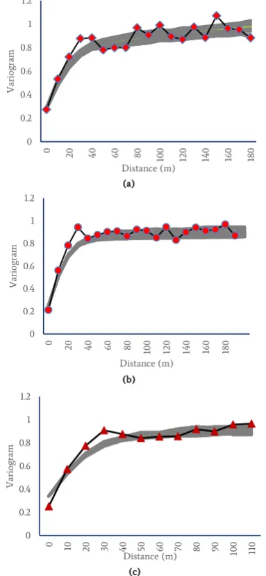
Fig. 6. The comparison of statistical parameters of samples data (horizontal line) and all realizations.
(a)
(b)
(c)
Fig. 7. Comparison between variograms of real data and realizations ((a) and (b) illustrate the horizontal direction at azimuth 0° and 90° respectively and (c) at
vertical direction).
0 0.2 0.4 0.6 0.8 1 1.2
0 20 40 60 80
10
0
120 140 160 180
Va
ri
og
ra
m
Distance (m)
0 0.2 0.4 0.6 0.8 1 1.2
0 20 40 60 80
10
0
120 140 160 180
Va
ri
og
ra
m
Distance (m)
0 0.2 0.4 0.6 0.8 1 1.2
0 10 20 30 40 50 60 70 80 90
10
0
11
0
Va
ri
og
ra
m
Ore grade histogram plot for input sample data and a random realization of SGS and for OK are presented in Fig. 8. It can be apperceived from these plots that due to the smoothing effect, the variance of the Kriging estimations is less than variance existed in the original data and simulated realizations. Comparison of the
distributions from the realizations with the samples data shows that the histograms of individual realizations are very similar to the samples data and they have generated watchfully the cumulative probability distribution of the original data.
(a) (b) (c)
Fig. 8. Ore grade histogram plot, (a) for input sample data, (b) one random realization of SGS and (c) for OK.
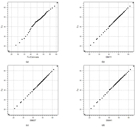
In addition, to compare the statistical parameters, Q–Q plots were prepared for the estimated model and individual realizations versus the samples data (Fig. 9). The Q–Q plot analysis procedure in this work gave
acceptable linear trends (located on the 45-degree line) between samples data and realizations. On the other hand, it can be seen that the OK method has a deviation from the mentioned trend line.
(a) (b)
(c) (d)
3.5.Determining ultimate pit in case of OK and SGS
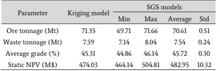
The process of open pit mine planning begins with the identification of ultimate limit of open pit mine. The available quality and quantity of ore are then defined within the ultimate pit limit, and this supply of material is represented in terms of grade-tonnage curves [32]. In this step of the study, considering the parameters given in Table 4, the economic block values were prepared for each grade model created by the Kriging and SGS methods. Utilizing the Lerches and Grossman (LG) algorithm [30], an ultimate pit for each case was recognized (Fig. 10), and the parameters including ore tonnage, waste tonnage, average grade, and NPV were calculated for each pit (Fig. 11).
Table 4. Required information in making an economic block model.
Parameter Quantity Unit
Ore Production 3 Million ton/ year
Overall pit slope 50 Degree
Density 0.038*Fe+1.86 ton/m3
Cut-off Grade 15 %
Recovery 90 %
Dilution 5 %
Ore mining cost 6 $/m3
Waste mining cost 4 $/m3
Crushing cost 1 $/ton
Discount rate 15 %
Product price 74 $/ton
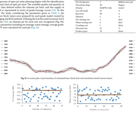
Fig. 10. A section plan of pit boundary of estimated-base (thick line) and simulation-based (narrow lines).
Fig. 11. Pit parameters obtained from kriging method (horizontal bar) and conditional simulations (points). Fig. 12 shows a comparison of grade-tonnage curves of the OK-based
pit and the simulation-based pits. Given the grade-tonnage curves and the economic parameters such as the price of metal, the operating costs, recovery, and the discount rate, the cutoff grade identifies the amount of ore and waste within the ultimate pit limit. Table 5 presents the details of final pits for both the conventional OK and the SGS method. Table 5 and Fig. 11 indicate that the pits resulted from OK gives more ore recovery as compared to the pit obtained from the SGS method. Nevertheless, a higher ore recovery cannot be considered merely as the economic index for selecting the optimum pit. In practice, the final decision is made according to the attainable NPV [5, 6, 34-37]. From NPV point of view, a large percentage of pits resulted from conditional simulation provide a higher NPV as compared to the OK-based pit.
Table 5. Details of final pits of both the conventional kriging method and the conditional simulations.
Parameter Kriging model SGS models
Min Max Average Std Ore tonnage (Mt) 71.35 69.71 71.66 70.61 0.51
Waste tonnage (Mt) 7.59 7.14 8.04 7.54 0.24
Average grade (%) 45.31 44.86 46.14 45.72 0.30 Static NPV (M$) 474.03 464.14 504.81 482.95 10.32
4.
Discussion and conclusions
This paper quantifies the ore grade uncertainty in ultimate pit determination and mine planning. In this study, the advantages of utilizing the SGS method over the conventional OK method in grade estimation and mine planning in uncertain condition was investigated in the Rezvan iron ore mine. An estimated orebody of an iron ore deposit was created using the OK method. Furthermore, by implementing the SGS method, 50 realizations of orebody were generated, and 30 realizations that proved high conformity of the simulation grade distribution to input data were selected. Through utilizing the LG algorithm, the ultimate pit for each case was recognized and the parameters including ore tonnage, waste tonnage, average grade, and NPV, were calculated for each pit. The obtained results were analyzed and the impact of ore grade uncertainty in open pit mine planning was identified.
From NPV point of view, a large percentage of pits based on SGS method, provide a higher NPV as compared to the OK-based pit. The OK-based pit shows more mineable ore and consequently lower stripping ratio as compared to the SGS-based pits. The results approved that using the OK-based planning can generate misleading outputs. This led to unrealistic optimism in mine planning and it could cause disappointing results. The smoothing effect generates unrealistic expectations of NPV and the stripping ratio in the mine’s design, along with ore production planning, pit limits and so on.
It can be understood from the achieved results that the traditional Kriging methods that are based on a single orebody model assumed to be the actual deposit in the ground being mined, the SGS-based model accounts for the uncertainty in the mineral supply from the deposit. In this regard, it can be concluded that these simulation methods are useful in quantitatively evaluating the uncertainty of economic and operational consequences of ultimate pit design and planning of open pit mines. Distributions of the ore grade in each of realizations can be used to analyze the data statistically for variances and to evaluate the uncertainty associated with various values in a probabilistic sense. The simulation methods can be used to improve the mine design of a mining project by considering the spatial distributions of ore grade and their uncertainty. The SGS method is more suited for these applications compared to the OK method. Subsequently, the resulting data can probabilistically assess the uncertainty. Application of the SGS method leads to substantially lower potential deviation from the production targets, which is reduced risk. In fact, the results obtained from the analysis have shown that which method can be used to develop the mining strategies that are less risk in relation to grade uncertainty. It is considered that if the main objective is providing a correct assessment of confidence intervals or a correct modeling of spatial continuity, then the simulation is the appropriate tool. The case study shows that multiple equally probable models of a deposit enable mine planners to assess the sensitivity of pit design and long-term production scheduling to ore grade uncertainty, and enable mine planners to produce more realistic mine designs.
Acknowledgments
The authors would like to acknowledge the valuable comments of the reviewers.
REFRENCES
[1] Ramazan, S., & Dimitrakopoulos, R. (2013). Production scheduling with uncertain supply: a new solution to the open pit mining problem. Optimization and Engineering, 14(2), 361-380. doi:10.1007/s11081-012-9186-2
[2] Chatterjee, S., Sethi, M., & Asad, M. (2016). Production phase and ultimate pit limit design under commodity price uncertainty. European Journal of Operational Research, 248(2), 658-667. doi:10.1016/j.ejor.2015.07.012
[3] Leite, A., & Dimitrakopoulos, R. (2014). Stochastic optimization of mine production scheduling with uncertain ore/metal/waste supply. Int. J. of Mining Science and Technology, 24(6), 755-762. doi:10.1016/j.ijmst.2014.10.004 [4] Benndorf, J., & Dimitrakopoulos, R. (2013). Stochastic
Long-Term Production Scheduling of Iron Ore Deposits Integrating Joint Multi-Element Geological Uncertainty. Journal of Mining Science, 49(1), 68–81.
[5] Gilani, S., & Sattarvand, J. (2016). Integrating geological uncertainty in long-term open pit mine production planning by ant colony optimization. Computers & Geosciences, 87(1), 31-40. doi:10.1016/j.cageo.2015.11.008
[6] Dimitrakopoulos, R. (2011). Stochastic optimization for strategic mine planning: A decade of developments. Journal of Mining Science, 47(2), 138–150.
[7] Rezaee, H., Asghari, O., & Yamamoto, J. (2011). On the reduction of the ordinary kriging smoothing effect. Journal of Mining & Environment, 2(2), 102-117.
[8] Deustech, C. V., & Journel, A. G. (1998). GSLIB: geostatistical software library and user’s guide. 2nd edn. Oxford University Press, New York.
[9] Ravenscroft, P. (1992). Risk analysis for mine scheduling by conditional simulation. Transactions of the Institution of Mining and Metallurgy. Section A. Mining Technology 101, A104–A108.
[10] Dimitrakopoulos, R. (1998). Conditional simulation algorithms for modelling orebody uncertainty in open pitoptimisation. Int J Min Reclamat Environ, 12, 173–179. [11] Smith, M., & Dimitrakopoulos, R. (1999). The influence of
deposit uncertainty on mine production scheduling. Int J Min Reclamat Environ, 173–178.
[12] Dimitrakopoulos, R., & Ramazan, S. (2004). Uncertainty-based production scheduling in open pit mining. transactions Society for Mining Metallurgy and Exploration, 106-112. [13] Godoy, M., & Dimitrakopoulos, R. (2004). Managing risk and
waste mining in long-term production scheduling of open-pit mines. transactions, 43-50.
[14] Ramazan, S., & Dimitrakopoulos, R. (2004). Traditional and New MIP Models for Production Scheduling with in-situ Grade Variability. International Journal Of Surface Mining, 18(2), 85-98.
[15] Menabde, M., & Froyland, G. (2004). Mining schedule optimisation for conditionally simulated orebodies. proceeding of the international symposium on ore body modelling and strategic mine planing, 347-352.
[16] Dimitrakopoulos, R., Farrelly, C., & Godoy, M. (2002). Moving forward from traditional optimization: grade uncertainty and risk effects in open-pit design. Trans. Instn Min. Metall, 82-88.
[18] Ramazan, S., & Dimitrakopoulos, R. (2007). Stochastic Optimisation of Long-Term Production Scheduling for Open Pit Mines With a New Integer Programming Formulation. Orebody Modelling and Strategic Mine Planning, 359-365. [19] Whittle, D., & Bozorgebrahimi, A. (2007). Hybrid pits-linking
conditional simulation and lerchs-grossmann through set theory. Orebody Modelling and Strategic Mine Planning, Spectrum Series, 323-328.
[20] Godoy, M., & Dimitrakopoulos, R. (2011). A risk quantification framework for strategic mine planning: Method and application. Journal of Mining Science, 47(2), 235-246.
[21] Goodfellow, R., & Dimitrakopoulos, R. (2012). Algorithmic integration of geological uncertainty in pushback designs for complex multiprocess open pit mines. Mining Technology, 1-12.
[22] Gholamnejad, J., & Moosavi, E. (2012). A new mathematical programming model for long-term production scheduling considering geological uncertainty. The Journal of The Southern African Institute of Mining and Metallurgy, 12(1), 77-81.
[23] Magri, E., Gonzalez, M., Couble, A., & Emery, X. (2003). The influence of conditional bias in optimum ultimate pit planning. APCOM 2003, South African Institute of Mining and Metallurgy, 429-436.
[24] Leite, A., & Dimitrakopoulos, R. (2007). A stochastic optimization model for open pit mine planning: application and risk analysis at acopper deposit. Transactions of the Institutions of Mining and Metallurgy, Section A: Mining Technology, 116, 109–118.
[25] Asghari, O., Soltani, F., & Bakhshandeh Amnieh, H. (2009). The comparison between sequential gaussian simulation (SGS) of Choghart ore deposit and geostatistical estimation through ordinary kriging. Aust J Basic Appl Sci, 3(1), 330–341. [26] Remy, N., Boucher, A., & Wu, J. (2009). Applied Geostatistics with SGeMS, A User's Guide. Cambridge University Press, Cambridge, United Kingdom, 264 pp.
[27] Dimitrakopoulos, R., & Luo, X. (2004). Generalized Sequential Gaussian Simulation on Group Size ν and Screen-Effect Approximations for Large Field Simulations. Mathematical Geology, 36(5), 567-591.
[28] Olea, A. O. (2006). A six-step practical approach to
semivariogram modeling. Stoch Environ Res Risk Assess, 20, 307–318. doi:10.1007/s00477-005-0026-1
[29] Karacan, C. O., Olea, R. A., & Goodman, G. (2012). Geostatistical modeling of the gas emission zone and its in-place gas content for Pittsburgh-seam mines using sequential Gaussian simulation. International Journal of Coal Geology, 90, 50-71. doi:10.1016/j.coal.2011.10.010
[30] Peng, X., Wanga, K., & Li, Q. (2014). A new power mapping method based on ordinary kriging and determination of optimal detector location strategy. Annals of Nuclear Energy, 68, 118–123.
[31] Rocha, M. M., & Yamamoto, J. K. (2000). Comparison Between Kriging Variance and Interpolation Variance as Uncertainty Measurements in the Capanema Iron Mine, State of Minas Gerais—Brazil. Natural Resources Research, 9(3), 223-235.
[32] Asad, M. W., & Dimitrakopoulos, R. (2012). Optimal production scale of open pit mining operations with uncertain metal supply and long-term stockpiles. Resources Policy, 37, 81-89. doi:10.1016/j.resourpol.2011.12.002
[33] Lerchs, H., & Grossmann, I. (1965). Optimum design of open-pit mines. Canadian Institute of Mining, Metallurgy and Petroleum Bulletin,, 58(1), 17−24.
[34] Chicoisne, R., Espinoza, D., Goycoolea, M., Moreno, E., & Rubio, E. (2012). A New Algorithm for the Open-Pit Mine production scheduling problem. Journal of Operations Research, 60(3), 517-528. doi:10.1287/opre.1120.1050 [35] Choudhury, S., & Chatterjee, S. (2014). Pit optimisation and
life of mine scheduling for a tenement in the Central African Copperbelt. Int. J. of Mining, Reclamation and Environment, 28(3), 200-213. doi:10.1080/17480930.2013.811802
[36] Aminul Haque, M., Topal, E., & Lilford, E. (2016). Estimation of Mining Project Values Through Real Option Valuation Using a Combination of Hedging Strategy and a Mean Reversion Commodity Price. Natural Resources Research, 1-13. doi:10.1007/s11053-016-9294-3