Open pit limit optimization using dijkstra’s algorithm

* Corresponding author. E-mail address: [email protected] (R. Rafiee).

Journal Homepage: ijmge.ut.ac.ir

Open pit limit optimization using dijkstra’s algorithm

Mehdi Najafi

_{, Ramin Rafiee}

_{, Seyed Mohammad Esmaiel Jalali}

a_{Department of Mining and Metallurgical Eng., Yazd University, Yazd, Iran}

b_{Faculty of Mining Engineering, Petroleum and Geophysics, Shahrood University of Technology, Iran}

A

B

S

T

R

A

C

T

In open-pit mine planning, the design of the most profitable ultimate pit limit is a prerequisite to developing a feasible mining sequence. Currently, the design of an ultimate pit is achieved through a computer program in most mining companies. The extraction of minerals in open mining methods needs a lot of capital investment, which may take several decades. Before the extraction, the pit limit, which influences the stripping ratio, damp locations, ore processing site and access routes, should be designed. So far, a large number of algorithms have been developed to optimize the pit limits. These algorithms are categorized into two groups: heuristic and rigorous. In this paper, a new approach is presented to optimize the pit limit based on Dijkstra’s algorithm which is based on mathematical relations. This algorithm was implemented on a 2D economic graph model and can find the true optimal solution. The results were compared with those from the dynamic programming (DP) algorithm. This algorithm showed to have less time complexity compared to the dynamic programming algorithm and to be easier to write dynamic computer programs.

Keywords : Graph Theory, Open Pit, Dijkstra’s Algorithm, Optimization, Dynamic Programing

1.

Introduction

Pit limit optimization has always been an essential issue for mine designers for economic reasons. Powerful computers developed during recent decades have assisted mining engineers in applying more accurate and complicated algorithms to the problem [1]. In recent years, open-pit areas have been optimized by making revenue block models and performing model-related optimization algorithms.

Many researchers have studied the ultimate pit limit optimization. Lerchs and Grossmann proposed a dynamic programming approach for two-dimensional final pit limit optimization [2]. Underwood and Tolwinski presented a mathematical programming for solving the same problem. They developed a network flow algorithm based on the dual to solve the ultimate pit problem [3]. Khalookakei et al. (2000) proposed a windows program for optimal open pit design with variable slope angles [4]. Askarinasab proposed an intelligent 3D interactive open pit based on the floating cone methods [5]. Sayadi et al. (2011) used a new artificial neural method to open-pit optimization [6]. kakaei et al. (2012) introduced a new algorithm for optimum open pit design based on the floating cone method [7].

Until now, many algorithms have been presented to determine the final open pit area of mines. The main purpose of these algorithms was finding a set of blocks to maximize the profit by extracting the blocks. These algorithms can be divided into two groups:

A: Heuristic algorithms

Heuristic algorithms refer to algorithms not supported by mathematical logic such as floating or moving cone method [8], floating cone II method [9], modified floating cone II methods [10], floating cone method III [7], Korobov algorithm [11], corrected form of the Korobov algorithm [12], genetic algorithm [13] and Network optimization [14]. However, these algorithms fail to guarantee the true

optimal solution, but they can usually reach the optimal point. These algorithms are fast and straightforward in their concept, computer coding, and implementation [15].

B: Rigorous algorithm

These algorithms, such as dynamic programming [2], are mathematically supported and take into account the area of hypothesized technical and economic constraints. Rigorous algorithms are generally able to guarantee the true optimal pit limits.

Regardless of being rigorous or heuristic, all of these algorithms define certain limits for the pit to be mined. The validity of the solution, indeed, depends on the validity of the type of algorithm used.

This paper aims to optimize the pit limits area using Dijkstra’s algorithm. Since Dijkstra’s algorithm is based on graph theory, the theory was used for simulation of block models. Then, 2D revenue block models of open pit area were explained and then the results of accuracy and performance were compared with the results of the dynamic programming algorithm.

2.

Graph theory

Conceptually, a graph is formed with vertices and edges connecting the vertices. However, in a formal definition, a graph is a pair of sets (V, E), where V is the set of vertices and E is the set of edges formed by pairs of vertices. E is a multiset; in other words, its elements can occur more than once so that every element has a multiplicity. Often, we label the vertices with letters. As an example, the graph depicted in Fig. 1 has vertex set V= {a, b, c, d, e, f} and edge set E = {(a, b), (b, c), (c, d), (c, e), (d, e), (e, f)} [16].

A subject that has many applications in a graph is the exploration of the shortest or longest path from one vertex to another vertex. Such a path should be a straightforward path. Finding the shortest or longest path is an optimization problem that the optimum value may be either

Article History:

a minimum or a maximum value.In the shortest path, the minimum length is an optimal solution value [16].

Fig. 1. An example of graph [16].

The optimization problem of open-pit mining using the graph model is the maximization of economic profit and the optimal path shows the maximum economic value of the extraction area.

3.

Dijkstra’s algorithm

Dijkstra's algorithm (or Dijkstra's Shortest Path First algorithm, SPF algorithm) is an algorithm for finding the shortest paths between nodes in a graph, which may represent, for example, road networks. It was conceived by the computer scientist Edsger W. Dijkstra in 1956 and was published three years later [17, 18]. For a given source node in a graph, the algorithm finds the shortest path between that node and the others. It can also be used for finding the shortest paths from a single node to a single destination node by stopping the algorithm once the shortest path to the destination node has been determined. Two sets are maintained in Dijkstra's algorithm; one set contains vertices included in the shortest path tree, the other set includes vertices not yet included in the shortest path tree. At every step of the algorithm, a vertex that is in the other set (the set of not yet included) and has a minimum distance from the source is found. Fig. 2 shows the detailed steps used in Dijkstra’s algorithm to find the shortest path from a single source vertex to all

other vertices [18]. These steps are as follows:

Step 1- Mark Vertex 1 as the source vertex. Assign a cost zero to Vertex 1.

Step 2- For each of the unvisited neighbors (Vertex 2, Vertex 3 and Vertex 4), calculate the minimum cost as min (current cost of vertex under consideration, the sum of the cost of vertex 1 and connecting edge). Mark Vertex 1 as visited, in the diagram we border it black.

Step 3- Choose the unvisited vertex with minimum cost (vertex 4) and consider all its unvisited neighbors (Vertex 5 and Vertex 6) and calculate the minimum cost for both of them.

Step 4- Choose the unvisited vertex with minimum cost (vertex 2 or vertex 5, here we chose vertex 2) and consider all its unvisited neighbors (Vertex 3 and Vertex 5) and calculate the minimum cost for both of them. Now, the current cost of Vertex 3 is [4] and the sum of the cost of Vertex 2 and the cost of edge (2,3) is 3 + 4 = [7]. The minimum of 4, 7 is 4. Hence, the cost of vertex 3 will not change. By the same argument, the cost of vertex 5 will not change. We mark vertex 2 as visited, and all costs remain the same.

Step 5- Choose the unvisited vertex with minimum cost (vertex 5) and consider all its unvisited neighbors (Vertex 3 and Vertex 6) and calculate the minimum cost for both of them. Now, the current cost of Vertex 3 is [4], and the sum of the cost of Vertex 5 and the cost of edge (5,3) is 3 + 6 = [9]. The minimum of 4, 9 is 4. Hence the cost of vertex 3 will not change. Now, the current cost of Vertex 6 is [6] and the sum of the cost of Vertex 5 and the cost of edge (3,6) is 3 + 2 = [5]. The minimum of 6, 5 is 45. Hence the cost of vertex 6 changes to 5.

Step 6- Choose the unvisited vertex with the minimum cost (vertex 3) and consider all its unvisited neighbors (none). Then mark it visited. Step 7- Choose the unvisited vertex with the minimum cost (vertex 6) and consider all its unvisited neighbors (none). then mark it visited.

a b

c d

e f

a b

c d

e f

a b

c d

Fig. 2. Computing the shortest paths using Dijkstra’s algorithm [18]. The performance of Dijkstra’s algorithm compared to mathematical

logic algorithms are relatively good and acceptable. Time complexity was used for investigating the performance of algorithms. In Dijkstra’s algorithm, the time complexity is n2 _{and is estimated according to}

Equation 1 [18].



 

 









_{ }

2 3 4 ...

1 2

... 2 1

2

TC n n n

n n

n



      

 

    (1)

where, n is the number of vertexes.

However, Dijkstra’s algorithm is usually used for finding the shortest path in a graph model. In this paper, Dijkstra’s algorithm was used to compute the longest path (maximum economic value) in the graph model by applying some corrections to the algorithm procedure. Since there is no loop in each probable path and the graph contains only a simple path in the simulated graph model, this goal can be obtained.

4.

Pit Limit Optimization

Since common optimization criteria are based on the maximum benefit achievement, revenue block models are used for determining the optimal area in most algorithms. In order to build a block model of the mining area, the deposit and a part of surrounding rocks of the mine were considered as a large block containing the whole mineralized areas. Then, the blocks were divided into smaller parts and the estimated grade was assigned to the blocks. In this way, the 2D conventional economic block model was built based on the economic data and the mining method [19]. The flow chart of calculating the limit of the open-pit area using Dijkstra’s algorithm is shown in Fig. 3.

Fig. 3. The flow chart of calculating the limit of the open-pit area using Dijkstra’s algorithm.

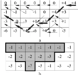
In order to illustrate the application of Dijkstra’s algorithm to optimize open-pit mining, a two-dimensional economic block model was created as shown in Fig. 4-a and also the cumulative revenue block model, as shown in Fig. 4-b. In this model, the economic value of each block is equal to the economic value of block plus the total economic

value of the blocks which are placed on top of the block. In this block model (Fig. 4-b), the blocks had the same size and the final slope of the open pit was considered 1:1 (45 degrees). The purpose of open-pit mining optimization is the maximization of the economic value of the extraction area. In open-pit mining, the length of the optimal path shows the value of the maximum extraction area.

a: Primary revenue block model -1 +1 -1 -1 -1 -1 -1 -2 -2 +3 -2 -2 +2 -2 -3 -3 +1 -3 +7 -3 -3 -1 +1 -1 -1 -1 -1 -1 -3 -1 +2 -3 -3 +1 -3 -6 -4 +3 -6 +4 -2 -6

b: Cumulative revenue block model Fig. 4. 2D revenue block model.

The two-dimensional revenue block model was used to build the ore graph model. The overall geometry and all paths in the graph model are based on the revenue block model and are defined by considering the technical and geometrical limitations of the extraction method. In order to develop the graph model based on the revenue block model, every corner of the blocks was considered as a vertex of the graph and the lines of blocks were considered as crests. In fact, each crest indicates a relationship between a block and other ones, which are located at the back and front of the block. Accordingly, the weight of each crest shows the cumulative economic value of the blocks that are placed on top of the crest. Fig. 5 shows a block of revenue block model and a part of the corresponding simulated graph. In this graph model, if the crest has upward concavity and the center of the block is placed on the top, it can be concluded that the economic value of the block is considered in the calculation of crest weight (crest Y2 in Fig. 5). It is clear that in this stage,

the weight of this crest and the horizontal crest, which connect the V2

and V3 vertices, are equal.

Fig. 5. Simulated block using the graph model.

In this study, the following assumptions are considered to simulate the block model using the graph model as shown in Fig. 4:

B: In order to show the connection between the blocks, three crests are drowned from each block to the others in the next column. One crest is connected to the block on the top row and the other one is connected to the next block on the same row and the final crest is connected to the block on the bottom row. Using this model, the limitation of open-pit mining is simulated when the final slop is considered 1:1.

C: In the graph model, the value of each crest represents the cumulative economic value of blocks that are placed above it. D: In this model, the value of each vertex is related to the previous

vertex. Fig. 6 shows how to assign value to each vertex in the graph by using the value of the previous vertex. For this purpose, the value of three previous vertices of each vertex in the previous column (top vertex, vertex in the same row, and the bottom vertex) are summed with the value of crests that entered to the vertex. The maximum calculated number is selected as the value of the vertex (Fig. 6-A). If the values of the two crests are the same, both crests are selected (Fig. 6-B). A graph is created using the block model with a cumulative value and by the valuation of the existing crests. In the next step, the value of each vertex that represents the economic value of the corresponding pit can be calculated.

Fig. 6. Valuation of each vertex in the simulated graph of the block model. The block model in Fig. 4 was simulated as a weighted graph and solved using Dijkstra’s algorithm. The weighted graph is shown in Fig. 7. The crests used for the valuation of vertices are depicted as continuous lines and the other ones are shown as dashed lines.

Fig. 7. Block model simulated using Dijkstra’s algorithm.

According to Dijkstra’s algorithm, the largest number in the last column is selected to determine the optimal area (Fig. 7). The optimal open pit mining area can be achieved by following the vertices which lead to the chosen crest. Nodes with the largest value represent the maximum economic value of the open-pit mining area. In this example, the obtained optimal value was equal to +4 units. In Fig. 7, the bold vertices show the maximum economic value corresponding to the optimal pit limit. The optimal area of mining on the block model is shown in Fig. 8 which was adjusted based on the results of Fig. 7.

Fig. 8. Optimal block model limit using Dijkstra’s algorithm.

4.1.Validity of the solution example

The dynamic programming (DP) algorithm was used for the validation of the proposed algorithm. The DP algorithm is one of the most popular methods in operation research to find the optimal solution in optimization problems [2]. For the first time, Lerchs and Grossmann used a dynamic programming method to design final open-pit mines in the two-dimensional state [2]. In order to validate the results of Dijkstra’s algorithm, the dynamic programming algorithm was performed on the example presented in Fig. 4. As shown in Fig. 9, the result of the dynamic programming was the same as those obtained from Dijkstra’s algorithm. It should be noted that the mainlimitation of Dijkstra's algorithmis that it cannot provide proper results for the graphs having negative weighed edges when used for the shortest path. However, in this research, it was used to compute the longest path (maximum economic value) in the graph model by applying some corrections to the algorithm procedure. Therefore, this limitation was resolved.

Fig. 9. The solution of 2D economic block model using the DP approach.

5.

Conclusion

Dijkstra and dynamic programming algorithms are often used for solving optimization problems. Dijkstra’s algorithm, in comparison with the dynamic programming algorithm, offers a simpler procedure and efficient solution. However, in dynamic programming, a dynamic character is used to divide the sample into smaller samples. In Dijkstra’s algorithm, however, the samples are not divided into smaller samples.

Both algorithms provide a two-dimensional optimal pit limit but since time complexity of dynamic programming algorithm is higher than that of Dijkstra's algorithm, it is better to use Dijkstra’s algorithm for determining the optimal pit limit..

REFERENCES

[1] Jalali S, Ataee-Pour M, Shahriar K (2006): Pit Limit Optimization Using Stochastic Process. CIM Bulletin 99, 1-11 [2] Lerchs H, Grossmann IF (1965): Optimum design of open pit

mines. Mining Bull 58, 47-54

[3] Underwood R, Tolwinski B (1998): A mathematical programming viewpoint for solving the ultimate pit problem. European Journal of Operational Research 107, 96-107 [4] Khalokakaie R, Dowd P, Fowell R (2000): A Windows

program for optimal open pit design with variable slope angles. International Journal of Surface Mining, Reclamation and Environment 14, 261-275

[5] Askarinasab H 2006: Intelligent 3D interactive open pit planning and optimization, Ph. D. Dissertation, Department of Civil and Enviromental Engineering, Edmonton, Alberta, Canada).

optimization in 3D using a new artificial neural network. Archives of Mining Sciences 56, 389-403

[7] Kakaie R (2012): A new algorithm for optimum open pit design: Floating cone method III. Journal of Mining and environment 2, 118-125

[8] Carlson TR, Erickson JD, O’Brain D, Pana MT (1966): Computer techniques in mine planning. Mining Engineering 18, 53-56

[9] Hochbaum DS, Chen A (2000): Performance analysis and best implementations of old and new algorithms for the open-pit mining problem. Operations Research 48, 894-914

[10] Khalokakaie R (2006): Optimum open pit design with modified moving cone II methods. Journal of engineering in Tehran university 4, 297-307

[11] David M, Dowd P, Korobov S (1974): Forecasting departure from planning in open pit design and grade control, 12th APCOM Symposium Colorado School of Mines, pp. F131-F153 [12] DowdPA O (1993): Open pitoptimization part1: The extraction pitdesign. Transactions of The Institution of mining and metallurgy 102, A95

[13] Denby B, Schofield D (1994): Open-pit design and scheduling

by use of genetic algorithms. Transactions of the Institution of Mining and Metallurgy. Section A. Mining Industry 103 [14] Khodayari AA (2013): A New Algorithm for Determining

Ultimate Pit Limits Based on Network Optimization. International Journal of Mining and Geo-Engineering 47, 129-137

[15] Kim Y (1978): Ultimate pit limit design methodologies using computer models—The state of the art. Mining engineering 30, 1454-1459

[16] Neapolitan R (2014): Foundations of Algorithms. Jones & Bartlett Learning

[17] Black P (2005): Greedy algorithm. Dictionary of Algorithms and Data Structures (online), US National Institute of Standards and Technology, February 2005

[18] Cormen TH, Leiserson CE, Rivest RL, Stein C (2001): Greedy algorithms. Introduction to algorithms 1, 329-355