www.geosci-instrum-method-data-syst.net/5/521/2016/ doi:10.5194/gi-5-521-2016
© Author(s) 2016. CC Attribution 3.0 License.
Optimized merging of search coil and fluxgate data for MMS
David Fischer1,5, Werner Magnes1, Christian Hagen1, Ivan Dors2, Mark W. Chutter2, Jerry Needell2, Roy B. Torbert2, Olivier Le Contel3, Robert J. Strangeway4, Gernot Kubin5, Aris Valavanoglou1, Ferdinand Plaschke1,
Rumi Nakamura1, Laurent Mirioni3, Christopher T. Russell4, Hannes K. Leinweber4, Kenneth R. Bromund6, Guan Le6, Lawrence Kepko6, Brian J. Anderson7, James A. Slavin8, and Wolfgang Baumjohann1
1Space Research Institute, Austrian Academy of Sciences, Graz, Austria
2Space Plasma/Magnetospheric Physics, University of New Hampshire, Durham, USA
3Laboratoire de Physique des Plasmas – UMR7648, CNRS/École Polytechnique/UPMC/Univ. Paris Sud/Obs. de Paris,
Paris, France
4Institute of Geophysics and Planetary Physics, University of California, Los Angeles, USA
5Signal Processing and Speech Communication Laboratory, Graz University of Technology, Graz, Austria 6Goddard Space Flight Center, NASA, Greenbelt, USA
7Applied Physics Laboratory, John Hopkins University, Laurel, USA
8Climate and Space Sciences and Engineering, University of Michigan, Ann Arbor, USA
Correspondence to:David Fischer ([email protected])
Received: 14 April 2016 – Published in Geosci. Instrum. Method. Data Syst. Discuss.: 6 June 2016 Revised: 19 September 2016 – Accepted: 30 September 2016 – Published: 17 November 2016
Abstract. The Magnetospheric Multiscale mission (MMS) targets the characterization of fine-scale current structures in the Earth’s tail and magnetopause. The high speed of these structures, when traversing one of the MMS spacecraft, cre-ates magnetic field signatures that cross the sensitive fre-quency bands of both search coil and fluxgate magnetome-ters. Higher data quality for analysis of these events can be achieved by combining data from both instrument types and using the frequency bands with best sensitivity and signal-to-noise ratio from both sensors. This can be achieved by a model-based frequency compensation approach which re-quires the precise knowledge of instrument gain and phase properties. We discuss relevant aspects of the instrument de-sign and the ground calibration activities, describe the model development and explain the application on in-flight data. Fi-nally, we show the precision of this method by comparison of in-flight data. It confirms unity gain and a time difference of less than 100 µs between the different magnetometer in-struments.
1 Introduction
The MMS mission (Magnetospheric Multiscale; Burch et al., 2015) is comprised of four satellites that are used to measure plasma processes in the Earth’s magnetosphere. The main mission target is the exploration of magnetic reconnection. To support measurements down to electron scales, the satel-lites are flying in a tight formation with distances down to 10 km. One of the main measurement quantities used to char-acterize plasma processes is the magnetic field. It is measured by three instruments which are part of the MMS FIELDS suite (Torbert et al., 2014): the analog fluxgate magnetome-ter (AFG), the digital fluxgate magnetomemagnetome-ter (DFG) and the search coil magnetometer (SCM). As the measured plasma structures can have speeds from 10 to 1000 km s−1, high measurement accuracy in both magnetic field magnitude and timing is required over a wide frequency range, e.g., to cal-culate speed and direction of a front crossing the tetrahedron satellite configuration.
frequen-cies and correspond to a low pass with low filter order and a corner frequency around 30 Hz. Therefore, fluxgate data are typically used for scientific analysis without any compensa-tion of the frequency-dependent gain and phase characteris-tics.
The search coil magnetometer is suitable for measuring much higher frequencies, but its sensitivity at lower frequen-cies is limited by the underlying induction principle. Its fre-quency response represents a transfer function of higher or-der and requires compensation based on ground calibration measurements (Le Contel et al., 2014).
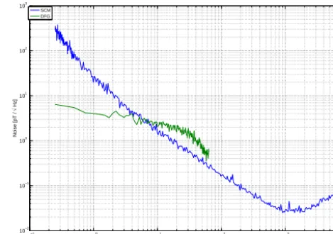
A noise floor comparison, which partly reflects the fre-quency response, is shown in Fig. 1. The plot compares the digital output of the DFG with the analog output from the SCM. The frequency range of equal noise floor is between 3 and 6 Hz, although this may vary across different instru-ment impleinstru-mentations. With the wide frequency range of plasma events mentioned above, it is desirable to have a com-mon merged product that combines the best data of both in-struments, i.e., all available frequency bands with lowest pos-sible noise floor. This is particularly useful for observations of electron diffusion regions and thin current sheets which feature signatures in the frequency range from 0.5 to 20 Hz (Torbert et al., 2014).
A similar approach was already used on magnetic field data from the Cluster and Themis missions, but in both cases it was based on limited on-ground frequency response calibration and usage of in-flight data for calibration. The SCM frequency characteristics were in principle known (Cornilleau-Wehrlin et al., 1997; Roux et al., 2008), but the knowledge of absolute time was limited. The knowledge of the frequency response of the fluxgates (Balogh et al., 1997; Auster et al., 2008) was limited to discrete frequency points in amplitude and low accuracy on end-to-end phase and tim-ing information. Mergtim-ing for data analysis was therefore only possible using this limited data and in-flight compar-ison (Alexandrova et al., 2004). Furthermore, comparative calibration of the SCMs was done by matching to fluxgate data at very low frequencies, which are not influenced by the fluxgate low pass characteristic (Robert et al., 2014).
Only the precise knowledge of the magnitude and phase response of both instrument types allows for accurate merg-ing of the respective data, keepmerg-ing intact phase and gain re-lations between different frequency components of the ob-served magnetic signatures. Therefore the shape of the sig-natures is preserved in the merged data product, as higher frequency components of steeper slopes stay phase aligned. Hence, the merged data are well suited for the analysis of internal fine structures of magnetic signatures as well as for high precision determinations of dipolarization front speed and direction by multi-spacecraft timing analysis. In addi-tion, the comparative calibration of gain and alignment be-tween SCM and AFG/DFG is massively improved in flight. Without the precise knowledge of their frequency responses either data with low signal-to-noise ratio (SNR) from the
10−1
100
101
102
103
104
10−2
10−1
100
101
102
103
Frequency [Hz]
Noise [pT /
√
Hz]
SCM DFG
Figure 1.Comparison of search coil (SCM) and fluxgate (DFG)
noise floor.
SCM (i.e., at the satellite spin frequency) or data with lit-tle phase knowledge from the fluxgate magnetometers have to be used for comparative calibration. This results in align-ment errors and inaccurate gain factors. With this knowledge, data from the complete common frequency band can be used and areas with good SNR can be selected.
The MMS FIELDS team invested significant efforts in in-strument design and test to ensure that end-to-end timing and frequency response information is already available from on-ground calibration. Design efforts include a common master clock and synchronization, which enables sampling of SCM, AFG and DFG with constant phase relation, as well as high precision time stamping. The target of these efforts was to reach an absolute time tagging accuracy of 100 µs across the full bandwidth despite the heterogeneous architecture of the instruments. This required common clocks and synchroniza-tion, as instruments are sampled by different means. AFG and DFG are sampled by their own electronics, whereas the SCM is sampled by the digital signal processing unit (DSP; Ergun et al., 2016). In both cases, depending on downlink data rate, digital filters for sample rate conversion are also applied, which also needs to be taken into account for time tagging.
2 Approach
Characterization of an unknown system is done by using known input signals, measuring the system response and cre-ating a model using both signals. For magnetometers the in-put signal has to be a magnetic field stimulus and the system response is the digital measurement result. Since both instru-ment types can be considered as linear and time-invariant for the case of a merged data product, it is possible to describe them with a model based on finite (FIR) or infinite impulse response filters (IIR). A suitable magnetic field stimulus can, for example, be created by a solenoid coil system. Ampli-tude and phase of the magnetic field are linked to the applied current.
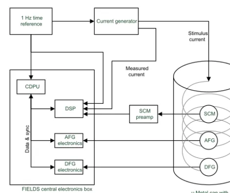
2.1 On-ground calibration and measurement setup Figure 2 shows a block diagram of the setup used for the fre-quency response calibration. All magnetic field sensors of the FIELDS instrument suite were placed in a mu-metal can and the stimulus signal was applied using a current generator and a solenoid coil. AFG and DFG were digitized by the respec-tive front-end electronics, while SCM signals first passed through a preamplifier and were then sampled by the DSP unit. The data streams were then processed by the FIELDS central data processing unit (CDPU).
The current generator and the CDPU were synchronized by a common 1 Hz time reference clock. All data recorded within FIELDS were time stamped relative to this reference. Furthermore all instruments within FIELDS were synchro-nized using common master and synchronization clocks. A more detailed description of this mechanism is available in the FIELDS instrument paper (Torbert et al., 2014).
The current generator that was constructed for this test is able to drive an arbitrary waveform current. It is generated by an internal digital signal generator. This signal genera-tor is operated at a sampling frequency of 4096 Hz, which is synchronized to the reference. This sampling clock is derived from a 67 MHz master clock internal to the current generator, but instead of using a fixed divider, additional clock cycles are added (or subtracted) as required to keep it synchronous to the 1 Hz time reference. These added clock cycles must be considered as artificial jitter, which in principle creates addi-tional noise in the stimulus signal. The maximum amplitude of this noise can be calculated by using the maximum possi-ble signal change within the maximum jitter time. For a jitter of 15 ns and a maximum signal frequency of 1024 Hz this results in an SNR of approximately 80 dB, which was suffi-ciently low for this purpose. As every real current source will produce small differences between desired and achieved cur-rent, an additional current measurement was mandatory. A comparison of the generated current and the 1 Hz time refer-ence signals shows a time deviation in the sub-microsecond range.
1 Hz time reference
SCM preamp
DFG electronics
AFG electronics
Current generator
DSP
Stimulus current
SCM
AFG
DFG
μ-Metal can with solenoid coil FIELDS central electronics box
CDPU
D
at
a
&
sy
n
c
Measured current
Figure 2.Test setup for instrument frequency response
measure-ments.
The current stimulus was driven through a solenoid coil in a mu-metal shielding, which attenuates external fields dur-ing the measurement. The influence of this coil/can system is minimal in the frequency range of interest from DC to 512 Hz; therefore the generated field could still be consid-ered as proportional to the measured current.
The stimulus waveforms used for testing need to cover the whole frequency range of interest. Commonly used test sig-nals for identifying unknown frequency responses are dis-crete frequency sines (using interpolation in between), sine sweeps and noise signals. Discrete and sweep sine signals have the advantage that the signal frequency for any given time is known and therefore all signals with different fre-quencies can be removed by bandpass filtering. However, longer measurement times are needed to excite all frequen-cies. Noise measurements excite all frequencies within a short period of time, but this method is sensitive to all ad-ditional noise sources within the analyzed frequency band. However, any uncorrelated noise can be reduced by longer measurements and averaging.
0 10 20 30 40 50 60 10−1
100
Gain
0 10 20 30 40 50 60
7.5 8 8.5 9 9.5 10 10.5 11 11.5 12
Frequency [Hz]
Phase delay [ms]
DFG Y AFG Y Sine DFG Y Sine AFG Y
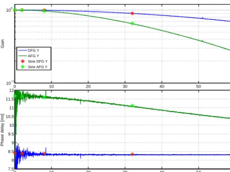
Figure 3.Frequency response of AFG and DFG measured with FFT
estimation method and sine signals. FFT length is 4096; overlap is 1023; rectangular window; data duration of 5 min.
In addition to the internal measurement of the current gen-erator, a voltage fully representative to the current stimulus was connected to a DSP voltage channel. This way, the cur-rent was also recorded synchronously to the FIELDS clock and so it could be used in later stages without the need for fur-ther resampling or time shifting. Additionally, this resulted in faster data transfer and easier data formatting.
2.2 Results of on-ground calibration
Using data from the first test, which was the digitizing of the time reference signals, it was possible to measure the delay introduced in sampling and time stamping of the DSP voltage channels by comparing the sampled waveform of the refer-ence clock and its time stamp. As the 1 Hz time referrefer-ence is giving the reference for the beginning of a full second, the clock edge within the sampled waveform should ideally be time stamped with this second. The measured deviation from the expected delay was less than 7 µs.
The results of the second test based on the sine signals delivered a highly accurate measurement of gain and phase at discrete frequencies and an initial approximation of the frequency response, for both the magnetic field instruments and the current measurement via the DSP voltage channel.
These first two tests showed that the DSP voltage channels had sufficiently flat frequency response and that the knowl-edge on timing accuracy was better than 1 µs. The later noise tests were therefore conducted using the current measure-ments of the DSP channels, as this resulted in reduced ef-fort in calculations. The additional delay of these channels was accounted for in all further tests. For verification pur-poses, both the sine and time reference measurements were included in all further test series to ensure that no changes occurred in the setup.
100
101
102
103
10−3 10−2
10−1
100
Gain
SCM Y SCM sine Y
100 101 102 103
−300 −200 −100 0 100 200
Phase [deg]
Frequency [Hz]
Figure 4.Frequency response of SCM measured with FFT
esti-mation method and sine signals. FFT length is 32 768; overlap is 32 767; rectangular window; data duration of 5 min.
The resulting data of the third test with applied noise sig-nals were used to create an initial estimate of the full in-strument frequency responses. This estimate can be found by dividing the fast Fourier transform (FFT) of stimulus and instrument measurements, which is the frequency domain equivalent of deconvolution.
Unfortunately, this method is not necessarily delivering an estimate that is fully representative for the system. The FFT method implies that a single transform window only contains the convolution of the transfer function and a stimulus. In re-ality the beginning of each FFT window contains a part of the response to previous stimulus data and a part of the re-sponse to the current stimulus is truncated. In addition, noise and distortion within the window are also considered as part of the frequency response. The problem of previous as well as truncated response data can be minimized by choosing a sufficiently large FFT length and by using windowing, over-lapping and averaging. The problem of measurement noise is more complicated. Although normal noise can be reduced by averaging, this is not the case for systematic distortion like powerline tones (50/60 Hz and harmonics). In this case the resulting estimate would have a changed frequency re-sponse at the respective frequencies. The FFT-based estimate can therefore not be used as a model.
slightly different characteristic due to the differences in ana-log elements.
Figure 4 shows the lower end of the expected SCM band-pass characteristic, which also matches the reference mea-surements taken by the SCM team in Chambon-la-Forêt (Le Contel et al., 2014). The frequency response for higher frequencies was not measured, as this was not required for the merged 1024 Hz data product.
The absolute timing of the FFT estimates was calculated by adding the delays of the DSP voltage channels known from the first two tests. A comparison between FFT estimate with added delay and the sine measurements, which do not include the current measurement via the DSP channel, shows good agreement and is therefore verifying the correct han-dling of delays in the DSP voltage channels.
2.3 Model development
The SCM model was chosen according to a theoretical model from the SCM team (Le Contel et al., 2014, Appendix A). As parts of the frequency transfer function of this model are far above the frequency band of interest, the model was reduced to a second-order IIR filter-based model and a fractional sam-ple Lagrange delay. Equation (1) shows the continuous time representation of the filter, which was converted to discrete time using the bilinear transform.
h(s)=
Gω1
1s
1 ω2s
1 ω1s+1
1 ω2s+1
(1)
The IIR model was then optimized to fit the measurement results in frequency domain, using a complex least mean square error fit (Eq. 2).
ω1,2=arg minE
n
HFFT(f )−F T h z, ω1,2 2
o
(2) Inversion of this optimized model is not directly possible, as it is not minimum phase (Oppenheim et al., 1999) – which means that the inverted model is unstable and has poles out-side of the unit circle. This is also visible by the differentiat-ing feature of the SCM. If this feature would be inverted, the resulting integrator would produce infinite values even with small DC inputs. As the lower parts of the spectrum are not used in the later merged product, it is possible to design a similar IIR transfer function with nonzero DC gain and min-imum phase property by just adding a small additional coef-ficient, thus changing the original numerator polynomial to have all poles within the unit circle. The resulting inverse model is a low shelving filter with a DC gain of 220 dB, which is close to the unmodified model for all frequencies above 0.1 Hz.
The main contributor to the frequency response of the DFG is the digital averaging filter used for the DFG internal downsampling (Magnes et al., 2003). Also, this filter cannot be considered as minimum phase and does not allow direct
0 20 40 60 80 100 120
−0.3 −0.2 −0.1 0 0.1 0.2 0.3 0.4
n
h [n]
MMS1 AFG axis 1
0 20 40 60 80 100 120
−0.6 −0.4 −0.2 0 0.2 0.4
n
h [n]
MMS1 DFG axis 1
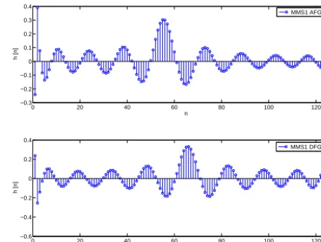
Figure 5.Exemplary impulse response of fluxgate compensation
filter model.
inversion. However, since only the spectral part below 64 Hz is used in the final 1024 Hz product, the properties of an in-version filter are irrelevant above these frequencies. This fact leaves some degrees of freedom for an optimization solution. The basic model in this case is a 128th-order FIR model that was derived using a Wiener–Hopf solution (Haykin, 2002). This method delivers a model that converts the input stimu-lus to a model output signal which tracks the real instrument measurements with minimum mean square error.
For the DFG this principle was inverted by exchanging in-put and outin-put, thus creating an inverse model that can di-rectly be applied on instrument data to reconstruct the “orig-inal” magnetic field data. Additionally, the instrument mea-surement data are compensated for the delay before model-ing, as otherwise the model would have to resemble both de-lay and frequency response of the instrument. Keeping these delays within the model would in principle only cause a shift of the model coefficients by adding zero coefficients at the beginning. This addition would increase the filter order that is used for optimization and instead of keeping these coef-ficients at zero, an optimal solution would try to model just the instrument noise to get to a minimum error. Introducing a time shift is therefore reducing model order and is avoiding coefficients that just model the noise.
The same approach, although with different delay com-pensation, was used on the AFG data. In this case the charac-teristic part of the filter is the analog low pass of the feed-back regulation loop, which also introduces non-constant group delay. The respective modeling process of each instru-ment was applied individually to each of the instruinstru-ment axes. An exemplary impulse response of the compensation filter model for AFG and DFG is presented in Fig. 5.
differ-0 50 100 150 200 250 300 350 400 450 500 0.9
1 1.1 1.2 1.3 1.4 1.5 1.6
Gain ratio
Δ FFT
Δ Reference
0 50 100 150 200 250 300 350 400 450 500 −0.1
−0.05 0 0.05 0.1
Δ
d
e
la
y
[
m
s
]
Frequency [Hz]
Figure 6.Gain ratio and delay difference between SCM frequency
response model and FFT estimate as well as analog reference cali-bration.
0 10 20 30 40 50 60
0.95 1 1.05
Gain ratio
0 10 20 30 40 50 60
−0.1 −0.05 0 0.05 0.1
Δ
de
la
y
[
m
s
]
Frequency [Hz]
Δ FFT
Figure 7.Gain ratio and delay difference between AFG frequency
response model and FFT.
ences between FFT-based results, model response and refer-ence calibration (Le Contel et al., 2014). The SCM model comparison in Fig. 6 shows the presence of powerline noise as peaks in amplitude and phase, both in the FFT (60 Hz) and the reference (50 Hz) measurements. These peaks are absent in the models and are therefore visible as differences in the comparison. The constant delay between reference and FFT as well as model measurements is due to the fact that the SCM reference calibration was only done using the analog sensor output and does not include all digital delays intro-duced by sampling.
Data from DFG and AFG presented in Figs. 7 and 8 show a very good match between model and FFT-based frequency response measurement results and, for DFG, also with the theoretical values of the digital averaging filter. The remain-ing delay variation of around 20 µs is well below the 100 µs
0 10 20 30 40 50 60
0.95 1 1.05
Gain ratio
0 10 20 30 40 50 60
−0.1 −0.05 0 0.05 0.1
Δ
de
la
y
[
m
s
]
Frequency [Hz]
Δ FFT
Δ Theory
Figure 8.Gain ratio and delay difference between DFG frequency
response model and FFT estimate as well as theoretical digital filter response.
goal. It is caused by the limited length FIR implementation, which could be corrected by a filter of higher order – but this has disadvantages, as shown in the next paragraphs.
The last step of model creation was to normalize the mod-els to the results of regular on-ground gain calibration of the instrument teams. For the fluxgates this was done by setting the DC gain to one, so DC calibration would be unchanged. For the SCM it was done by matching the gains of model and on-ground reference calibration around 1 kHz.
The filter-based instrument models require an initial filter settling time that is dependent on the filter impulse response length. Data from this period need to be removed from the final data product and therefore produce a data gap. This is of special concern for MMS high sampling rate data, as only short data bursts are transmitted and a loss of many data points cannot be tolerated. Some of this could be mitigated by prefilling with data from lower sampling frequencies, but this process is complex, as multiple frequency response com-pensation is involved. The best solution is therefore the use of limited length filter functions.
IIR filter was used as SCM model. A replacement by an FIR model is planned in the future.
Data from both instruments are merged with a crossover filter that is weighting different spectral parts of the instru-ments according to their properties. An optimum crossover filter set would weigh the different frequency components of the signal based on a comparison of instrument sensitiv-ity, noise floor and possible distortion. These weights can be considered as filter function with variations in frequency do-main. A transform of a filter function with high variability will result in a high-order filter function, which will again cause data loss due to filter settling. We therefore chose to implement a windowed FIR low and high pass filter based on the sinc function, which is simply using DFG/AFG data up to 4 Hz and SCM data above. The sinc function also pro-vides the advantage that design of the respective complemen-tary filter is a simple subtraction from the Dirac delta. This means the sum of the two filters is unity gain. Furthermore, comparison to unfiltered signals is simple due to its constant group delay property.
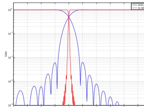
Here the window length also has to be matched to an acceptable data loss due to filter settling. With larger win-dow size stopband attenuation increases, passband ripple de-creases and the crossover characteristic has a steeper slope. Figure 9 shows an example of two filter sets with different window lengths and the resulting differences in attenuation and crossover slope. For initial merging and comparison the 16 385 point filter was used, but in later mission phases with shorter data bursts this will be changed to 2049 points or less, depending on available burst data length.
3 Application
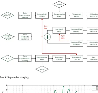
The final process of merging, which is suitable for automated application, is shown in the data flow diagram in Fig. 10. Apart from the already discussed crossover filters and model-based frequency response compensation, a few more blocks are present in this diagram. The uncalibrated data files from all instruments (called L1A data according to MMS defini-tion) are passed through a block that handles fragmentation, as data files can have gaps and contiguous data can be dis-tributed over several files.
The resampling block includes antialiasing filters and con-verts the different data products to the final product rate of 1024 Hz. The first remaining sample in the decimated data product of SCM is selected by looking for the closest neigh-bor in the fluxgate data, thus minimizing the time distance between those samples. This reduces the amount of time shift needed to synchronize the data to a common sample time ba-sis.
The blocks for timestamp updates and fractional delays are two separate parts of a common mechanism. Fractional de-lays (less than a sampling period) are required to align data to a common time basis and to compensate absolute time
de-0 1 2 3 4 5 6 7 8 9 10
10−4 10−3
10−2
10−1
100
Frequency [Hz]
Gain
2049 points 16 385 points
Figure 9.Frequency response of two merging filters with different
filter lengths.
lays. A pure fractional time shift can be achieved by inter-polation, but this would require infinite data. All realizable methods use limited time interpolation which affects gain and phase at higher frequencies.
In the time stamp update block only the time stamp is corrected by the known delays, while in the fractional de-lay block the fluxgate data are interpolated to the time line of the search coil data. This way all time shifts are applied with a single fractional delay filter and the influence on gain and phase is minimized. This shift was implemented as La-grange filter and its overall spectral influence is minimal, as the higher frequency parts of the fluxgate spectrum are not used in the final merged data product.
Resample @ 1024 Hz
Compensation filter Data
Fragmentation Handling
Calibration @1024 Hz
Coordinate transform Timestamp
update
+
Finalcoordinate transforms
Compensation filter
Timestamp update
Resample @ 1024 Hz Data
fragmentation handling
Gain calibration Coordinate transform Crossover filter
highpass Model
Model Merged
product AFG/DFG
SCM
Sync
data Crossover filter
lowpass Fractional
delay
Sync data
Figure 10.Data flow block diagram for merging.
59 59.5 60 60.5 61 61.5 62
−4 −2 0 2 4
BX
[nT]
2015−08−15 12:55:xx Time [s]
DFG SCM
Figure 11.Comparison of MMS 3 frequency compensated data of DFG and SCM in time domain with band limitation from 4 to 64 Hz.
After merging, the data are finally transformed to the target coordinate system, i.e., geocentric solar ecliptic or magneto-spheric.
4 Evaluation
The merged data of about 2 months were used for evaluation of the data product, as tracking of small-scale differences in time, alignment and gain required statistics on high rate burst data, which were not available at all times due to operational constraints.
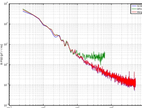
A first time domain comparison (Fig. 11) in the band from 4 to 64 Hz shows good visual agreement between compen-sated data from SCM and DFG. A power spectral analysis (Fig. 12) shows the improved sensitivity of the merged prod-uct for higher frequencies. For lower frequencies the spec-trum is dominated by the natural signal, as burst data are only available in regions of scientific interest that show field ac-tivity. This is in fact even the case for the higher part of the spectrum that also exceeds the noise floor of the SCM.
A more accurate analysis of the quality of the compen-sation models can be achieved by comparing relative gain and phase between compensated SCM and DFG data. The re-sult of this comparison is shown in Fig. 13. The calculations for these figures were done by dividing the FFT spectra of the individual axes, which should ideally result in unity gain and zero phase for a system with perfect frequency response compensation. Data were analyzed using FFT windows with a length of 2048 points and averaging over 10 min. Only data sets with relevant amplitudes in the frequency range 10– 64 Hz were taken into account, i.e., sets that have more than 10 000 points above a 100 pT magnetic field threshold with an average of at least 150 pT.
The gain plot in Fig. 13 shows a gain factor that is close to unity up to at least 30 Hz. A clear interpretation above this frequency is difficult, as the noise increases massively. This is due to the low amplitudes of natural signals in this fre-quency range. These signals barely exceed the noise floor of the fluxgate, thus resulting in a poor SNR.
10−1 100 101 102 103 10−2
10−1
100 101
102
103
Frequency [Hz]
B PSD [pT /
√
Hz]
SCM DFG Merged
Figure 12.PSD comparison of SCM and DFG on MMS1 during a
quiet field period on 20 September 2015, 06:33:31 UTC.
quality of timing determination is in this case better, as a tim-ing error would result in a linear phase trend. For comparison purposes the time accuracy goal of 100 µs was converted to linear phase trends and added to the plots. Comparing this limit to the measurement result shows no linear trends in this order of magnitude and verifies that time stamping accuracy is definitely better than 100 µs in the investigated frequency band.
In addition to timing, alignment and gain were also com-pared by minimizing the differences between DFG and SCM measurements using linear combination of the different axes with a 3×3 alignment matrix. The result showed that the angle mismatch between DFG and SCM was in the order of 0.5 to 1◦. This fits well to the expected differences, as SCM initial calibration assumes perfect orthogonality and align-ment, while fluxgate data have full alignment and orthogo-nality calibration in place. The result of these comparison will be added to the SCM calibration flow in the near future.
5 Conclusion
The common effort of the MMS FIELDS team allowed us to create frequency response models for the FIELDS mag-netic field instruments that are based on full end-to-end on-ground calibration. Using these models, good agreement be-tween data from search coil and fluxgate magnetometers was achieved and data could be merged to a common product with a timing precision better than 100 µs. Furthermore, the developed methods are suitable for automated processing.
With the frequency response compensated data, alignment and gain corrections for the search coil were also gener-ated by comparison with the in-flight calibrgener-ated fluxgate data. The resulting merged magnetometer provides a new basis for analysis of scientific events which contain frequencies ranges that are spread across two instruments.
10 15 20 25 30 35 40 45 50 55 60 −20
−15 −10 −5 0 5 10 15 20
Phase difference [degree]
Frequency [Hz]
100 us phase equivalent
10 15 20 25 30 35 40 45 50 55 60 0.7
0.8 0.9 1 1.1 1.2
Gain ratio
Figure 13.Comparison of gain and phase for MMS 1 SCM and
DFG data.
6 Data availability
MMS inflight data are available at the MMS science data cen-ter at https://lasp.colorado.edu/mms/sdc/. Data are partially subject to export control or access restrictions. Access can be requested at the University of New Hampshire (ground cali-bration) or at the MMS Science Data Center (inflight data).
Acknowledgements. The dedication and expertise of the
Magneto-spheric Multiscale (MMS) development and operations teams are greatly appreciated. Work at JHU/APL, UCLA, UNH and SwRI was supported by NASA contract number NNG04EB99C. The French involvement (SCM) on MMS is supported by CNES and CNRS.
We acknowledge the use of burst L1A data from digital and analog fluxgate magnetometers and search coil magnetome-ters. The data are stored at the MMS Science Data Center https://lasp.colorado.edu/mms/sdc/ and are publicly available. The Austrian part of the development, operation and calibration of the DFG was financially supported by rolling grant of the Austrian Academy of Sciences and the Austrian Space Applications Pro-gramme with the contract number FFG/ASAP-844377.
Edited by: V. Korepanov
References
Alexandrova, O., Mangeney, A., Maksimovic, M., Lacombe, C., Cornilleau-Wehrlin, N., Lucek, E. A., Décréau, P. M. E., Bosqued, J.-M., Travnicek, P., and Fazakerley, A. N.: Cluster ob-servations of finite amplitude Alfvén waves and small-scale mag-netic filaments downstream of a quasi-perpendicular shock, J. Geophys. Res., 109, A05207, doi:10.1029/2003JA010056, 2004. Auster, H. U., Glassmeier, K. H., Magnes, W., Aydogar, O., Baumjohann, W., Constantinescu, D., Fischer, D., Fornacon, K. H., Georgescu, E., Harvey, P., Hillenmaier, O., Kroth, R., Lud-lam, M., Narita, Y., Nakamura, R., Okrafka, K., Plaschke, F., Richter, I., Schwarzl, H., Stoll, B., Valavanoglou, A., and Wiede-mann, M.: The THEMIS Fluxgate Magnetometer, Space Sci. Rev., 141, 235–264, doi:10.1007/s11214-008-9365-9, 2008. Balogh, A., Dunlop, M. W., Cowley, S. W. H., Southwood, D.
J., Thomlinson, J. G., Glassmeier, K. H., Musmann, G., Lühr, H., Buchert, S., Acuña, M. H., Fairfield, D. H., Slavin, J. A., Riedler, W., Schwingenschuh, K., and Kivelson, M. G.: The Cluster Magnetic Field Investigation, Space Sci. Rev., 79, 65– 91, doi:10.1023/A:1004970907748, 1997.
Burch, J. L, Moore, T. E., Torbert, R. B., and Giles, B. L.: Magneto-spheric Multiscale Overview and Science Objectives, Space Sci. Rev., 199, 5–21, doi:10.1007/s11214-015-0164-9, 2015. Cornilleau-Wehrlin, N., Chauveau, P., Louis, S., Meyer, A., Nappa,
J. M., Perraut, S., Rezeau, L., Robert, P., Roux, A., De Villedary, C., De Conchy, Y., Friel, L., Harvey, C. C., Hubert, D., Lacombe, C., Manning, R., Wouters, F., Lefeuvre, F., Parrot, M., Pinçon, J. L., Poirier, B., Kofman, W., and Louarn, P.: The Cluster Spatio-Temporal Analysis of Field Fluctuations (STAFF) Experiment, Space Sci. Rev., 79, 107–136, doi:10.1023/A:1004979209565, 1997.
Ergun, R. E., Tucker, S., Westfall, J., Goodrich, K. A., Malaspina, D. M., Summers, D., Wallace, J., Karlsson, M., Mack, J., Bren-nan, N., Pyke, B., Withnell, P., Torbert, R., Macri, J., Rau, D., Dors, I., Needell, J., Lindqvist, P.-A., Olsson, G., and Cully, C. M.: The Axial Double Probe and Fields Signal Process-ing for the MMS Mission, Space Sci. Rev., 199, 167–188, doi:10.1007/s11214-014-0115-x, 2016.
Haykin, S.: Adaptive Filter Theory, 4th Edn., Prentice Hall, Upper Saddle River, NJ, USA, 2002.
Le Contel, O., Leroy, P., Roux, A., Coillot, C., Alison, D., Bouab-dellah, A., Mirioni, L., Meslier, L., Galic, A., Vassal, M. C., Tor-bert, R. B., Needell, J., Rau, D., Dors, I., Ergun, R. E., West-fall, J., Summers, D., Wallace, J., Magnes, W., Valavanoglou, A., Olsson, G., Chutter, M., Macri, J., Myers, S., Turco, S., Nolin, J., Bodet, D., Rowe, K., Tanguy, M., and de la Porte, B.: The Search Coil Magnetometer for MMS, Space Sci. Rev., 199, 257– 282, doi:10.1007/s11214-014-0096-9, 2014.
Magnes, W., Pierce, D., Valavanoglou, A., Means, J., Baumjo-hann, W., Russell, C. T., Schwingenschuh, K., and Graber, G.: A sigma delta fluxgate magnetometer for space applications, Meas. Sci. Technol., 14, 1003–1012, doi:10.1088/0957-0233/14/7/314, 2003.
Oppenheim, A. V., Schafer, R. W., and Buck, J. R.: Discrete Time Signal Processing, 2nd Edn., Prentice Hall, Upper Saddle River, NJ, USA, 1999.
Robert, P., Cornilleau-Wehrlin, N., Piberne, R., de Conchy, Y., La-combe, C., Bouzid, V., Grison, B., Alison, D., and Canu, P.: CLUSTER-STAFF search coil magnetometer calibration – com-parisons with FGM, Geosci. Instrum. Method. Data Syst., 3, 153–177, doi:10.5194/gi-3-153-2014, 2014.
Roux, A., Le Contel, O., Coillot, C., Bouabdellah, A., de la Porte, B., Alison, D., Ruocco, S., and Vassal, M. C.: The Search Coil Magnetometer for THEMIS, Space Sci. Rev., 141, 265–275, doi:10.1007/s11214-008-9455-8, 2008.
Russell, C. T., Anderson, B. J., Baumjohann, W., Bromund, K. R., Dearborn, D., Fischer, D., Le, G., Leinweber, H. K., Leneman, D., Magnes, W., Means, J. D., Moldwin, M. B., Nakamura, R., Pierce, D., Plaschke, F., Rowe, K. M., Slavin, J. A., Strange-way, R. J., Torbert, R., Hagen, C., Jernej, I., Valavanoglou, A., and Richter, I.: The Magnetospheric Multiscale Magnetometers, Space Sci. Rev., 199, 189–256, doi:10.1007/s11214-014-0057-3, 2014.