Assessment of wavelet-based spatial verification by means of
a stochastic precipitation model (wv_verif v0.1.0)
Sebastian Buschow, Jakiw Pidstrigach, and Petra Friederichs Institute of Geosciences, University of Bonn, Bonn, Germany
Correspondence:Sebastian Buschow ([email protected]) Received: 4 April 2019 – Discussion started: 24 April 2019
Revised: 27 June 2019 – Accepted: 5 July 2019 – Published: 5 August 2019
Abstract. The quality of precipitation forecasts is difficult to evaluate objectively because images with disjointed fea-tures surrounded by zero intensities cannot easily be com-pared pixel by pixel: any displacement between observed and predicted fields is punished twice, generally leading to better marks for coarser models. To answer the question of whether a highly resolved model truly delivers an improved representation of precipitation processes, alternative tools are thus needed. Wavelet transformations can be used to summa-rize high-dimensional data in a few numbers which charac-terize the field’s texture. A comparison of the transformed fields judges models solely based on their ability to predict spatial structures. The fidelity of the forecast’s overall pat-tern is thus investigated separately from potential errors in feature location. This study introduces several new wavelet-based structure scores for the verification of deterministic as well as ensemble predictions. Their properties are rigorously tested in an idealized setting: a recently developed stochastic model for precipitation extremes generates realistic pairs of synthetic observations and forecasts with prespecified spatial correlations. The wavelet scores are found to react sensitively to differences in structural properties, meaning that the ob-jectively best forecast can be determined even in cases where this task is difficult to accomplish by naked eye. Random rain fields prove to be a useful test bed for any verification tool that aims for an assessment of structure.
1 Introduction
Typical precipitation fields are characterized by large empty areas, interspersed with patches of complicated structure. Forecasts of such intermittent patterns are difficult to
ver-ify because we cannot compare them to the observations in a grid-point-wise manner: if a given rain feature is forecast perfectly, but slightly displaced, point-wise verification will punish the error twice, once at the points where precipitation is missing and once at the points where it was erroneously placed. The correctly predicted structure is not rewarded in any way. Following the advent of high-resolution numeri-cal weather predictions, this effect, known asdouble penalty (Ebert, 2008), has motivated the introduction of numerous new spatial verification tools.
In a comprehensive review of the field, Gilleland et al. (2009) identified four main strategies that deal with the dou-ble penalty prodou-blem and supply useful diagnostic informa-tion on the nature and gravity of forecast errors. The clas-sification was updated to include an emerging fifth class in Dorninger et al. (2018). Proponents of the first strategy, the so-called neighbourhood approach, attempt to ameliorate the issue via successive application of spatial smoothing filters (Theis et al., 2005; Roberts and Lean, 2008). A second group of researchers including Keil and Craig (2009), Gilleland et al. (2010), and recently Han and Szunyogh (2018) explic-itly measure and correct displacement errors by continuously deforming the forecast into the observed field. A third pop-ular approach consists of automatically identifying discrete objects in each field and subsequently comparing the prop-erties of these objects instead of the underlying fields. Ex-amples from this category include the MODE technique of Davis et al. (2006) as well as the SAL technique by Wernli et al. (2008).
wavelet-based intensity-scale score of Casati et al. (2004), which decomposes the difference field between observation and forecast via thresholding and an orthogonal wavelet transformation. The final class newly identified by Dorninger et al. (2018) contains the so-calleddistance measures, which exploit mathematical metrics between binary images devel-oped for image processing applications. One example is Bad-deley’s delta metric, which was first employed as a verifica-tion tool in Gilleland (2011).
The basic idea of the method presented in this study, which can be classified as a scale-separation technique, is that er-rors, that neither relate to the marginal distribution nor to the location of individual features, should manifest themselves in the field’s spatial covariance matrix. Direct estimates of all covariances would require unrealistically large ensemble data sets or restrictive distributional assumptions. Following a similar approach to scale-separated verification, Marzban and Sandgathe (2009), Scheuerer and Hamill (2015), and Ek-ström (2016) therefore base their verification on the fields’ variograms. The variogram is directly related to the spatial auto-correlations (Bachmaier and Backes, 2011) but can be estimated from a single field under the assumption that pair-wise differences between values at two grid points only de-pend on the distance between those locations (the so-called intrinsic hypothesisof Matheron, 1963). Similarly one could require stationarity of the spatial correlations themselves, in which case the desired information is contained within the field’s Fourier transform. Both of these stationarity as-sumptions may be inadequate in realistic situations where the structure of the data varies systematically across the domain; for example, due to orographic forcing, the distribution of water bodies or persistent circulation features.
Weniger et al. (2017) have suggested an alternative ap-proach based on wavelets. The key result in this context comes from the field of texture analysis, where Eckley et al. (2010) proved that the output of a two-dimensional discrete redundant wavelet transform (RDWT) is directly connected to the spatial covariances. The crucial advantage of their ap-proach is that it merely requires the spatial variation of co-variances to be slow, not zero – a property known aslocal stationarity. After some initial experiments by Weniger et al. (2017), this framework has successfully been applied to the ensemble verification of quantitative precipitation forecasts by Kapp et al. (2018). Their methodology consists of (1) per-forming the corrected RDWT, following Eckley et al. (2010), to obtain an unbiased estimate of the local wavelet spectra at all grid points, (2) averaging these spectra over space, (3) re-ducing the dimension of these average spectra via linear dis-criminant analysis, and (4) verifying the forecast via the log-arithmic score.
In this study, we aim to expand on their pioneering work in several ways. Firstly, we argue that the aggregation method of simple spatial averaging is not the only sensible approach. An alternative is introduced which incidentally suggests a compact way of visualizing the results of the RDWT: instead
of aggregating in the spatial domain, we first aggregate in the scale domain by calculating the dominant scale at each lo-cation. Secondly, we use both kinds of spatial aggregates to introduce a series of new wavelet-based scores. In contrast to Kapp et al. (2018), we consider both the ensemble case and the deterministic task of comparing individual fields while avoiding the need for further data reduction. We furthermore demonstrate how to obtain a well defined sign for the error, indicating whether forecast fields are scaled too small or too large. The experiments performed to study the properties of our scores constitute another main innovation: the recently developed stochastic rain model of Hewer (2018) allows us to set up a controlled yet realistic test bed, where the differ-ences between synthetic forecasts and observations lie solely in the covariances and can be finely tuned at will. In con-trast to similar tests performed by Marzban and Sandgathe (2009) and Scheuerer and Hamill (2015), our data are physi-cally consistent and thus bear close resemblance to observed rain fields. Lastly, we consider the choice of mother wavelet in detail, using the rigorous wavelet-selection procedure of Goel and Vidakovic (1995). The sensitivity of all newly in-troduced scores to the wavelet choice is assessed as well.
The remainder of this paper is structured as follows. The stochastic model of Hewer (2018) is introduced in Sect. 2. Sections 3 and 4 respectively discuss the wavelet transforma-tion and spatial aggregatransforma-tion in detail. The general sensitivity of the wavelet spectra to changes in correlation structure is experimentally tested in Sect. 5. Based on these results, we define several possible deterministic and probabilistic scores in Sect. 6. In a second set of experiments (Sect. 7), we sim-ulate synthetic sets of observations and predictions and test our scores’ ability to correctly determine the best forecast. A comprehensive discussion of all results is given in Sect. 8.
2 Data: stochastic rain fields
In order to test whether our methodology can indeed detect structural differences between rain fields, we need a reason-ably large rain-like data set whose structure is, to some ex-tent, known a priori. Faced with a similar task, Wernli et al. (2008), Ahijevych et al. (2009), and others have employed purely geometric test cases. While those experiments are ed-ucational, we would argue that the simple, regular texture of such data bears too little resemblance with reality to consti-tute a sensible test case for our purposes. As an alternative, Marzban and Sandgathe (2009) considered Gaussian random fields, which have the advantage that the texture is more in-teresting and can be changed continuously via the parame-ters of the correlation model. However, since precipitation is generally known to follow non-Gaussian distributions, the realism of this approach is arguably still lacking.
field with non-zero values, i.e. the base rate. The velocity and its divergence are represented via the two-dimensional Helmholtz decomposition, which reads
v= ∇ ×9+ ∇χ ⇒ ∇ ·v= ∇2χ ,
where∇ ×9:=(−∂x9, ∂y9)T is the rotation of the
stream-function andχ is the velocity potential. The spatial process of P is thus completely determined by (9, χ , q)T, which we model as a multivariate Gaussian random field with zero mean and covariance matrix
Cov(9s, χs, qs)T, (9t, χt, qt)T
=
69,χ ,q·M(||b(t−s)||, ν ) . (2)
Here,t,s∈R2are two locations within the 2-D domain and M is the Matérn covariance function. The parameterb gov-erns the scale of the correlations and the smoothness parame-terνdetermines the differentiability of the paths. The matrix 69,χ ,q is set to unity for our experiments, meaning that the
velocity components and humidity are uncorrelated. Prelim-inary tests have shown that these parameters have negligible effects on the structural properties of the resulting rain fields. The covariances needed to simulate a realization of P via Eq. (1), i.e.
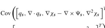
Cov
h
qs,∇ ·qs,∇χs− ∇ ×9s,∇2χs iT
h
qt,∇ ·qt,∇χt− ∇ ×9t,∇2χt iT
,
follow from Eq. (2) by taking the respective mean-square derivatives. In the special case where9,χ, andqare uncor-related, these three Gaussian fields, as well as the necessary first and second derivatives, can directly be simulated via the RMcurlfreemodel from theRpackageRandomFields (Schlather et al., 2013). While the underlying distributions of 9,χ andq are Gaussian, the precipitation process, consist-ing of non-linear combinations of the derived fields, can ex-hibit non-Gaussian behaviour. For further details, the reader is referred to Hewer et al. (2017), Hewer (2018), and refer-ences therein.
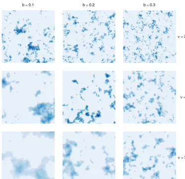
Figure 1 shows several realizations of P. Here, as in the rest of this study, we have normalized all fields to unit sum, thereby removing any differences in total intensity and allow-ing us to concentrate on structure alone. We recognize that the model produces realistic-looking rain fields, at least for moderately low smoothness (smallν) and large scales (small
the scalar parameterbby a rotation matrix), but the technical implementation remains a non-trivial problem. The search for a non-stationary version is an open research question in its own right.
3 The redundant discrete wavelet transform
The technical core of our methodology consists of project-ing the fields onto a series of so-called daughter wavelets ψj,l,u(r):R2→R, which are all obtained from a mother
waveletψ (r)via scaling byr→r/j, a shift byr→r−u and rotation in the direction denoted byl. Suchwavelet trans-forms, which generate a series of basis functions from a sin-gle motherψthat is localized in space and frequency, allow for an efficient analysis of non-stationary signals on a hierar-chy of scales and have attained great popularity in numerous applications. For a general introduction to the field, we rec-ommend Vidakovic and Mueller (1994) and Addison (2017). Before we can apply wavelets to our problem, we must choose a motherψand decide which values of{j, l,u}to al-low. Starting with the latter decision and guided by our desire to capture the field’s covariance structure, we follow Weniger et al. (2017) and Kapp et al. (2018) in choosing a redundant discrete wavelet transform (RDWT). In this framework, the shiftutakes on all possible discrete values, meaning that the daughters are shifted to all locations on the discrete grid. The scalej is restricted to powers of 2 and the daughters have three orientations with l=1,2,3 denoting the horizontal, vertical, and diagonal direction, respectively. The projection onto these daughter wavelets, for which efficient algorithms are implemented in theR package wavethresh(Nason, 2016), transforms a 2J×2Jfield into 3×J×2J×2J coef-ficients, one for each location, scale, and direction. Our deci-sion in favour of the RDWT is motivated by a relevant result proven in Eckley et al. (2010). Let
X(r)= X
allj,l,u Wj,l,u | {z }
weight
·ψj,l,u(r) | {z }
daughter
·ξj,l,u | {z }
noise
(3)
Figure 1.Example realizations of the stochastic rain model on a 128×128 grid for various choices of scaleband smoothnessν. The threshold T was chosen such that 20 % of the field has non-zero values.
a more condensed summary. The main result of Eckley et al. (2010) states that in the limit of an infinitely high spatial reso-lution, the autocovariances ofXcan directly be inferred from the squared weights |W|2. In analogy to the Fourier trans-form,|W|2is referred to as thelocal wavelet spectrum. Eck-ley et al. (2010) have furthermore proven that the squared coefficients of X’s RDWT constitute a biased estimator of this spectrum: due to the redundancy of the transform, the very large daughter wavelets all contain mostly the same in-formation, leading to spectra which unduly over-emphasize the large scales. The bias is corrected via multiplication by a matrix A−1 which contains the correlations between the ψj,l,u and thus depends only on the choice of ψ and the size and resolution of the domain. Away from the asymptotic limit, this step occasionally introduces negative values to the spectra, which have no physical interpretation and pose some practical challenges in the subsequent steps. Preliminary in-vestigations have shown that the abundance of thisnegative energysharply decreases with the smoothness of the wavelet ψand mostly averages out when mean spectra over the
com-plete domain are considered (cf. Appendix, Fig. A3). Apart from the bias correction, the corrected local spectra also need to be smoothed spatially in order to obtain a consistent esti-mate. The complete procedure, including the computation-ally expensive calculation ofA−1, is implemented in theR packageLS2W(Eckley and Nason, 2011).
Having decided on a type of transformation, we must se-lect a mother waveletψ. Our decision is restricted by the fact that the results of Eckley et al. (2010) have only been proven for the family of orthogonal Daubechies wavelets. These widely used functions, henceforth denotedDN, have
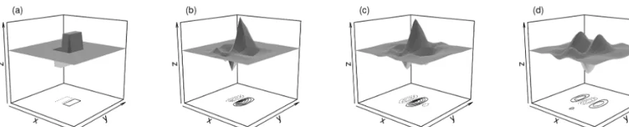
compact support in the spatial domain, increasing values of N indicate larger support sizes as well as greater smooth-ness. Smoother and hence more wave-like basis functions with better frequency localization are thus also more spread out in space. Figure 2 shows a few examples from this fam-ily.D1(panel a), the only family member that can be
Figure 2. Two-dimensional Daubechies daughter waveletsD1 and D2 (a, b), as well as least asymmetricD4 (c)and D8 (d), vertical orientation.
Kapp et al., 2018). For N >3, the constraints on smooth-ness and support length allow for multiple solutions, two of which are typically used: the extremal phase solutions are optimally concentrated near the origin of their support, while the least asymmetric versions have the greatest symmetry (Mallat, 1999). D1,2,3 belongs in both sub-families;
wher-ever a distinction is needed, we will label the two branches of the family asExPandLeA, respectively. Among these avail-able mother wavelets, we seek the basis that most closely re-sembles the data, thus justifying the model given in Eq. (3). To this end, we follow Goel and Vidakovic (1995) and rank wavelets by their ability to compress the original data: the sparser the representation (the more of the coefficients are negligibly small) in a given wavelet basis, the greater the similarity between basis functions and data. Relegating all details concerning this procedure to Appendix A, we merely note that the structure of the rain field, determined by the pa-rametersb andν, has substantially more impact on the effi-ciency of the compression than the choice of wavelet. Over-all, the least asymmetric version of D4(shown in Fig. 2c)
is most frequently selected as the best basis (28 % of cases), followed byD1andD2(21 % each). Unless otherwise noted,
we will therefore employ LeA4 in all subsequent experi-ments. Considering the relatively small differences between wavelets, we hypothesize that the basis selection should have only minor effects on the behaviour of the resulting verifica-tion measures – a claim which is tested empirically in Sect. 7.
4 Wavelet spectra spatial aggregation
The previous step’s redundant transform inflates the data by a factor of 3×J, meaning that a radical dimension reduction is needed before verification can take place. Throughout this study, we will always begin this process by discarding the two largest scales, which are mostly determined by boundary conditions, and averaging over the three directions. The latter step is unproblematic, at least for our isotropic test cases. Next, the resulting fields must be spatially aggregated in a way that eliminates the double-penalty effect.
The straightforward approach to this task consists of sim-ply averaging the wavelet spectra over all locations. The re-dundancy of the transform guarantees that this mean
spec-trum is invariant under shifts of the underlying field (Na-son et al., 2000), thereby allowing us to circumvent double-penalty effects. Kapp et al. (2018) have already demonstrated that the spatial mean contains enough information to confi-dently distinguish between weather situations in a realistic setting. In particular, the difference between organized large-scale precipitation and scattered convection has a clear signa-ture in these spectra – an observation that has recently been exploited by Brune et al. (2018), who defined a series of wavelet-based indices of convective organization using this approach. As mentioned above, we furthermore know that negative energy, introduced by the correction matrixA−1, mostly averages out in the spatial mean, provided that we choose a wavelet smoother thanD1(cf. Appendix, Fig. A3).
In spite of these desirable properties, there are two main issues which motivate us to consider an alternative way of aggregation: if we normalize the mean spectrum to unit total energy, its individual values can be interpreted as the fraction of totalrain intensityassociated with a given scale and direc-tion. It is easy to imagine cases where a very small fraction of the total precipitation area contains almost all of the total intensity and therefore dominates the mean spectrum. This is clearly at odds with the intuitive concept oftexture. Further-more, there is no obvious way of visualizing how individual parts of the domain contribute to the mean spectrum – if our visual assessment disagrees with the wavelet-based score, we can hardly look at all fields of coefficients at once in order to pinpoint the origin of the dispute. This second point leads us to introduce themap of central scalesC: for every grid point (x, y)within the domain, we setCx,y to the centre of mass
of the local wavelet spectrum. The resulting 2J×2J field of C∈(1, J )is a straightforward visualization of the redundant wavelet transform, intuitively showing the dominant scale at each location. Since the centre of mass is only well defined for non-negative vectors, all negative values introduced by the bias correction viaA−1are set to zero before computing C.
distribu-Figure 3.Logarithmic rain field(a)and corresponding map of central scales(b)from the stage II reanalysis on 13 May 2005. The field has been cut and padded with zeroes to 512×512, scales were calculated using the least asymmetricD4wavelet, only locations with non-zero
rain are shown. Panels(c)and(d)show the corresponding mean spectrum and scale histogram, respectively.
tion (Casati et al., 2004) and reduce the impact of single ex-treme events. We see a clear distinction between the large frontal structure in the centre of the domain (scales 6–7), the medium-sized features in the upper-left quadrant (scale 4– 5), and the very small objects on the lower right (scales≤4). As an alternative to the spatial mean spectrum (Fig. 3c), we can base our scores on the histogram ofC over all locations pooled together (Fig. 3d). Intuitively, this scale histogram summarizes which fraction of the total area is associated with features of various scales. We observe a clear bi-modal structure which nicely reflects the two dominant features on scales five and six.
5 Wavelet spectra sensitivity analysis
Before we design verification tools based on the mean wavelet spectra and histograms of central scales, it is instruc-tive to study what these curves look like and how they react to changes in the model parametersb,ν, andT from Eq. (1). Can we correctly detect subtle differences in scale? What are the effects of smoothness and precipitation area? To answer these questions, we begin by simulating 100 realizations of our stochastic model on a 128×128 grid, first keeping the smoothnessνconstant at 2.5 and varying the scalebbetween 0.1 and 0.5 (recall that large values ofbindicate small-scaled
features). For a second set of experiments, we simulate 100 fields with constantb=0.25 and varyνbetween 2.5 and 4. All of these fields are then normalized to unit sum (to elimi-nate differences in intensity), transformed and aggregated as described above.
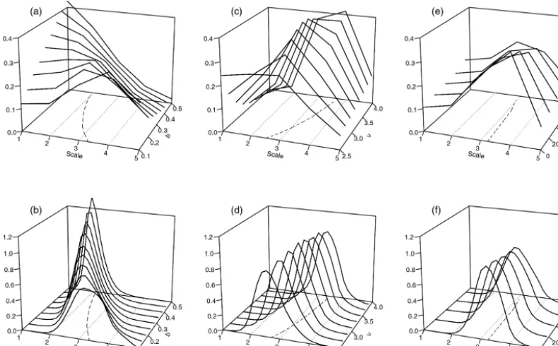
Figure 4a shows the spatial mean spectra, averaged over all directions and realizations, as a function of the scale parame-terb(on theyaxis). As expected, an increase inb monotoni-cally shifts the centre of these spectra towards smaller scales. Considering the experiment with variableν(panel c), we find that an increase in smoothness results in a shift towards larger scales. This is in good agreement with the visual impression we get from the example realizations in Fig. 1. The corre-sponding scale histograms are shown in Fig. 4b and d. We observe that their centres, corresponding to the expectation values of the central scales, are shifted in the same directions (and to a similar extent) as the mean spectra.
In addition to the shift along the scale axis, we observe that the two model parameters have a secondary effect on the shapes of the curves: a decrease inborνgoes along with flat-ter mean spectra – the energy is more evenly spread across scales. The histograms react similarly tob, larger scales co-inciding with greater variance, while changes inνhave only a minor impact on the histogram’s shape.
Figure 4.Mean spectra(a, c, e)and histograms of central scale(b, d, f), as functions of the scale parameterbatν=2.5(a, b), smoothness parameterνatb=0.25(c, d), and thresholdT atb=0.1 andν=2.5(e, f). Dashed lines in thex–y-plane indicate the respective curve centres of mass; dotted grey lines (parallel to theyaxis) were added for orientation.
characteristics are less clear: are fields with a larger fraction of precipitating area perceived to be scaled larger or smaller? To investigate this, we setb=0.1 andν=2.5 and vary the rain area between 10 % and 100 %. Figure 4e and f shows that the centres of the spectra and histograms hardly depend onT at all. The spread slightly increases with the threshold in both cases, but the changes are far more subtle than for the other two parameters.
In summary, we note that the two structural parameters ν andb have clearly visible effects on the mean spectra as well as the scale histograms. Metrics that compare the com-plete curves (as opposed to their centres alone) should be able to distinguish between errors in scale and smoothness since these characteristics have different effects on their location and spread. The effect of the thresholdT is only moderate in comparison, but could potentially compensate errors in the other two parameters, which may occasionally lead to coun-terintuitive results.
6 Wavelet-based scores
Motivated by the previous section’s results, we now intro-duce several possible scores, comparing the spectra and his-tograms of forecast and observed rain fields. Here, we con-sider the case of a single deterministic prediction, as well as ensemble forecasts.
6.1 Deterministic setting
of central scales (henceforthHemd) and the normalized,
spa-tially and directionally averaged, wavelet spectra (henceforth Spemd), respectively.
Being a metric, the EMD is positive and semi-definite and therefore yields no information on the direction of the error. We can obtain such a judgement by calculating, instead of the EMD, the difference between the respective centres of mass. For the histograms, this corresponds to the difference in expectation value. Rubner et al. (2000) have proven that the absolute value of this quantity is a lower bound of the EMD. Its sign indicates the direction in which the forecast spectrum or histogram is shifted, compared to the observa-tions. We have thus obtained two additional scores,Hcdand
Spcd, which are conceptually and computationally simpler
than the EMD versions and allow us to decide whether the scales of the forecast fields are too large or too small. 6.2 Probabilistic setting
When predictions are made in the form of probability dis-tributions (or samples from such a distribution), verification is typically performed using proper scoring rules (Gneiting and Raftery, 2007). Here, we treat scoring rules as cost func-tions to be minimized, meaning that low values indicate good forecasts. A functionSthat maps a probabilistic forecast and an observed event to the extended real line is then called a proper score when the predictive distribution F minimizes the expected value ofSas long as the observations are drawn from F. In this case, there is no incentive to predict any-thing other than one’s best knowledge of the truth.Sis called strictly properwhenF is the only forecast which attains that minimum. As mentioned above, Kapp et al. (2018) verified the spatial mean wavelet spectra via the logarithmic score, which necessitates a further dimension reduction step. In the interest of simplicity as well as consistency with our other scores, we employ the energy score (Gneiting and Raftery, 2007) instead, which is given by
En(F,y)=EF|X−y| −0.5EF|X−X0|, (4)
whereyis the observed vector,EF denotes the expectation
value under the multivariate distribution of the forecast F, andXandX0are independent random vectors with
distribu-tionF. Here, we substitute the observed mean spectrum fory and estimateF from the ensemble of predicted spectra. The resulting score, which we will denote as Spen, is proper in
the sense that forecasters are encouraged to quote their true beliefs about the distribution of the spatial mean spectra.
The two previously introduced scores based on the his-tograms of central scales can directly be applied to the case of ensemble verification by estimating the forecast histogram from all ensemble members pooled together. In this setting where two distributions are compared directly,proper diver-gences(Thorarinsdottir et al., 2013) take the place of proper scores: a divergence, mapping predicted and observed distri-butionsF andGto the real line, is called proper when its
expected minimum lies atF =G. The square ofHcd
corre-sponds to the mean value divergence, which is proper.Hemd
is a special case of the Wasserstein distance, the propriety of which is only guaranteed in the limit of infinite sample sizes (Thorarinsdottir et al., 2013). Whether or not these diver-gences are useful verification tools in the probabilistic case will be tested empirically in Sect. 7.
All of our newly proposed wavelet-based texture scores are listed in Table 1.
6.3 Established alternatives
In order to benchmark the performance of our new scores, we compare them to potential non-wavelet alternatives from the literature. A first natural choice is the variogram score of Scheuerer and Hamill (2015), which is given by
V (F,y)=
n
X
a,b=1
wa,b |ya−yb|p−EF[|Xa−Xb|p]2, (5)
where y, F, and X now correspond to the observed rain field, the distribution of the predicted rain fields, and a ran-dom field distributed according to the latter.a andbdenote two grid points within the domain. The weightswa,bcan be
used to change the emphasis on pairs with small or large dis-tances, while the exponentpgoverns the relative importance of single, extremely large differences. We include two ver-sions of this score in our verification experiment: the naive choicewa,b=1, p=2 (denoted V20 below) and the more
robust configurationwa,b= |ra−rb|−1,p=0.5 (Vw,5
be-low), whereradenotes the spatial location corresponding to
the indexa. Assuming stationarity of the data, we can effi-ciently calculate both of these scores by first aggregating the pairwise differences over all pairs with the same distance in space up to a pre-selected maximum distance.V20then
sim-plifies to the mean-square error between the two stationary variograms. The maximum distance is set to 20, which is a rough approximation of the range of the typical variograms of our test cases. Preliminary experiments have shown that this aggregation greatly improves the performances ofVw,5
andV20in all of our experiments. It furthermore allows us to
Spen energy score of the predicted mean spectra yes no
RMSE root-mean-square error between rain fields no yes Vw,5 variogram score,wa,b= |ra−rb|−1,p=0.5 yes yes
V20 variogram score,wa,b=1,p=2 yes yes
S object-based structure score of Wernli et al. (2008) yes yes
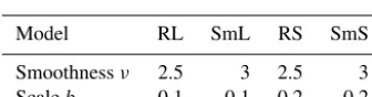
Table 2.Varying parameters in Eq. (2) for the four groups of artifi-cial ensemble forecasts.
Model RL SmL RS SmS
Smoothnessν 2.5 3 2.5 3 Scaleb 0.1 0.1 0.2 0.2
in our test cases. For the purposes of ensemble verification, we employ a recently developed ensemble generalization of SAL (Radanovics et al., 2018). Here, the ratio between max-imum and total predicted rain is averaged not only over rain objects, but also over the ensemble members.
Lastly, the naive root-mean-square error (RMSE) will be included in our deterministic verification experiment in order to confirm the necessity for more sophisticated methods of analysis.
7 Idealized verification experiments
For our first set of randomly drawn forecasts and observa-tions from the model given by Eq. (1), we keep the threshold T constant such that 20 % of the fields have non-zero values and select four combinations ofνandb, listed in Table 2.
The resulting texture is rough and large scaled (RL), smooth and large scaled (SmL), rough and small scaled (RS), and smooth small scaled (SmS). One realization for each of those settings is depicted in Fig. 1. In the following sections, we interpret random samples of these models as observations and forecasts, thus allowing us to observe how frequently the truly best prediction (the one with the same parameters as the observation) is awarded the best score.
7.1 Ensemble setting
Beginning with the synthetic ensemble verification experi-ment, we draw 100 realizations each from RL and RS as our observations. For every observation (200 in total), we is-sue four ensemble predictions, consisting of 10 realizations from RL, SmL, RS, and SmS, respectively. Only one of these
10-member ensembles thus represents the correct correla-tion structure while the other three are wrong in either scale, smoothness, or both. Observation and ensembles are com-pared via the three wavelet scoresHcd, Hemd, and Spen as
well as the established alternatives for ensemble forecasts, i.e.S,V20, andVw,5.
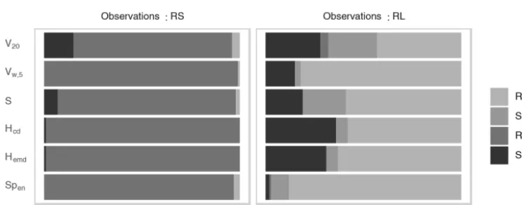
Figure 5 shows the resulting score distributions. All scores are best when small, except for the two-sided S and Hcd
where values near zero are optimal. Beginning with the case where the observations are drawn from RS (top row of Fig. 5), we observe that the four predictions are ranked quite similarly by all scores. Here, the correct forecast almost al-ways receives the best mark, while SmL, which is most dis-similar from RS, fares worst.S andHcdfurthermore agree
that all three false predictions are scaled too large. The task of determining the truly best forecast is substantially more com-plicated when the observations belong to RL (bottom row of Fig. 5): since SmS is both smoother and scaled smaller, the effects on the location of the spectra and histograms along the scale axis (cf. Fig. 4) compensate each other. These curves can therefore hardly be distinguished by their centres of mass alone. We recognize that RL and SmS consequently obtain similar values ofHcd, this score judging solely based on the
centres. The other two wavelet scores achieve better discrim-ination, as doesVw,5. Concerning the signs of the error, we
note thatS andHcd both consider RS too small and SmL
too large. For SmS,Hcdis only slightly negative, indicating
nearly correct scales.Sis less affected by the compensating effect of increased smoothness and determines more clearly that SmS is smaller-scaled than RL. Its overall success rate is, however, not significantly better than that ofHcd.
Figure 6 summarizes the ability of the six tested proba-bilistic scores to correctly determine the best forecast ensem-ble. As discussed above, all scores are very successful at de-termining correct forecasts of RS. In the alternative setting (observations from RL), SmS is the most frequent wrong an-swer, receiving the smallest (absolute) values ofV20,S,Hcd,
andHemdin more than a quarter of cases. In contrast to the
other scores, Spenhardly ever erroneously prefers SmS over
lead-Figure 5.Distribution of all probabilistic scores for each of the forecast ensembles corresponding to the four models from Table 2. Top row: observations drawn from RS. Bottom row: observations drawn from RL. Numbers denote the fraction of cases in which the forecast from the correct distribution received the best score.
Figure 6.Percentage of cases where each of the four ensembles corresponding to the models in Table 2 was deemed the best forecast, separated by score and the model of the observation.
ing to the overall lowest error rate (12 %) in this part of the experiment.
7.2 Deterministic setting
Having investigated the behaviour of our probabilistic scores, we now consider the deterministic case: how successfully can we determine the truly best forecast, given only a sin-gle realization? The set-up for this experiment is the same as before, only the size of the forecast ensembles is reduced from 10 to 1. Since the resulting scores naturally have greater variances than before, we increase the number of observa-tions to 1000 (500 each from RL and RS) in order to achieve similarly robust results. In addition to the four appropriate wavelet scores (Spemd, Spcd,HemdandHcd), we again
cal-culateVw,5andV20as well as theScomponent of the
orig-inal SAL score. To ensure that the verification problem is
sufficiently difficult, the root-mean-square error (RMSE) is included as a naive alternative as well.
Figure 7 reveals that correct forecasts are again easily identified by all of the wavelet-based scores when the ob-served fields belong to RS. As in the ensemble scenario, the main difficulty lies in the decision between SmS and RL in cases where the latter model generates the observations. The two EMD scores, which use the complete curves and not just their centres, clearly outperform the corresponding CD versions in this part of the experiment and detect RL correctly in the majority of cases.Vw,5is similarly
success-ful as the best wavelet-based score, faring marginally better than Spemd. The failure rates ofV20andSare again slightly
Figure 7.As Fig. 6, but for the deterministic verification experiment.
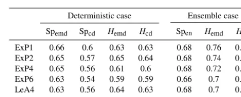
Table 3.Fraction of cases where the correct forecast received the best score for a range of extremal phase (ExP) and least asymmetric (LeA) Daubechies wavelets. LeA4 is the wavelet used for all other experiments in this study; ExP1 is the well-known Haar wavelet.
Deterministic case Ensemble case
Spemd Spcd Hemd Hcd Spen Hemd Hcd
ExP1 0.76 0.72 0.73 0.72 0.86 0.78 0.78 ExP2 0.83 0.73 0.8 0.77 0.92 0.82 0.83 ExP4 0.87 0.7 0.8 0.75 0.94 0.87 0.78 ExP6 0.87 0.7 0.82 0.73 0.94 0.86 0.74 LeA4 0.84 0.71 0.76 0.73 0.92 0.81 0.78 LeA6 0.86 0.69 0.76 0.69 0.94 0.88 0.8
the fact that the model with the largest, smoothest features (SmL) has the least potential for double penalties and thus fares best in a point-wise comparison; in fact, RMSE orders the four models by their typical features size, irrespective of the distribution of the observation.
7.3 Wavelet choice and bias correction
One obvious question to ask is whether or not the choice of the mother wavelet has a significant impact on the success rates in the two experiments discussed above. To address this issue, we repeat both the deterministic and the ensemble ver-ification processes for several Daubechies wavelets. Recall-ing the results of our objective wavelet selection (Sect. 3 and Appendix A), we expect no dramatic effects.
Table 3, listing the overall success rates for each tested wavelet, mostly confirms this expectation: in the determin-istic case, Spemd and Hemd are really only affected by the
choice between the Haar wavelet, which performs worst, and any of its smoother cousins. The two centre-based scores (SpcdandHcd) show hardly any wavelet dependence at all.
Sensitivities are overall slightly higher in the ensemble case. While D1 again appears to be the worst choice, there are
some differences between the other options, particularly for the two histogram scores. Generally speaking, the impacts
Table 4.As Table 3, but without the bias-correction step.
Deterministic case Ensemble case
Spemd Spcd Hemd Hcd Spen Hemd Hcd
ExP1 0.66 0.6 0.63 0.63 0.68 0.76 0.74 ExP2 0.65 0.57 0.65 0.64 0.68 0.74 0.76 ExP4 0.65 0.56 0.61 0.6 0.68 0.72 0.72 ExP6 0.63 0.54 0.59 0.59 0.66 0.7 0.71 LeA4 0.63 0.56 0.64 0.63 0.68 0.7 0.68 LeA6 0.63 0.55 0.62 0.61 0.66 0.69 0.68
of wavelet choice on our verification results are nonetheless rather limited, as long as the Haar wavelet is avoided.
To confirm that the bias correction following Eckley et al. (2010) is indeed a necessary part of our methodology, we re-peat these experiments without applying the correction ma-trixA−1. Without discussing the details (Table 4), we merely note that the success rates decrease substantially (depending on score and wavelet), meaning that bias correction generally cannot be skipped.
7.4 Perturbed thresholds
Next, we consider the case where forecast and observations are subject to random perturbations which are not directly re-lated to the underlying covariance model. One rather natural way of implementing this scenario consists of randomly per-turbing the thresholds, i.e. the fractions of the domain cov-ered by non-zero precipitation. In a realistic context, such random differences between forecast and observation could be associated with a displacement error which shifts unduly large or small parts of a precipitation field into the forecast domain.
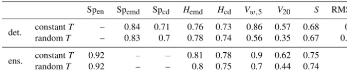
Table 5.Fraction of cases where the correct forecast received the best score. Top two rows: deterministic forecasts with and without perturbed threshold. Bottom: ensemble forecasts with and without perturbed thresholds.
Spen Spemd Spcd Hemd Hcd Vw,5 V20 S RMSE
det. constantT – 0.84 0.71 0.76 0.73 0.86 0.57 0.68 0.2 randomT – 0.83 0.7 0.78 0.74 0.56 0.35 0.67 0.22
ens. constantT 0.92 – – 0.81 0.78 0.9 0.62 0.75 – randomT 0.92 – – 0.8 0.75 0.7 0.44 0.74 –
the pairwise distances from which the stationary variogram is estimated. To test these hypotheses, we again repeat the two verification experiments, this time randomly varyingT such that the precipitation area, previously fixed at 20 %, is a uni-form random variable between 15 % and 25 % of complete domain.
Looking at the resulting success rates (Table 5), we find our expectations largely confirmed: while variations in the precipitation coverage hardly influence our wavelet-based judgement, Vw,5 andV20 seem to strongly depend on this
parameter, thus mostly losing their ability to determine the correct model. The performances of S and RMSE are only weakly influenced by variations inT.
8 Summary and discussion
The basic idea of this study is that the structure of precipita-tion fields can be isolated and subsequently compared using two-dimensional wavelet transforms. Building on the work of Eckley et al. (2010) and Kapp et al. (2018), we have ar-gued that the corrected, smoothed version of the redundant discrete wavelet transform (RDWT) is an appropriate tool for this task since it is shift invariant and has a proven asymptotic connection with the correlation function of the underlying spatial process. This approach is theoretically more flexible than Fourier- or variogram-based methods which make some form of global stationarity assumption, while our method re-lies on the substantially weaker requirement of local station-arity.
Before wavelet-transformed forecasts and observations can be compared to one another, the spatial data must be ag-gregated in a way that avoids penalizing displacement errors twice. Besides the proven strategy (Kapp et al., 2018) of av-eraging the wavelet spectra over all locations, we have newly introduced the map of central scales as a potentially inter-esting alternative: by calculating the centre of mass for each local spectrum, we obtain a matrix of the same dimensions as the original field, each value quantifying the locally domi-nant scale. Aside from the possibility of compactly visualiz-ing the output of the RDWT in a svisualiz-ingle image, the histogram of these scales can serve as an alternative basis for verifica-tion, emphasizing each scale based on the area in which it
dominates, rather than the fraction of total rain intensity it represents.
In order to rigorously test the sensitivity of these aggre-gated wavelet transforms to changes in the structure of rain fields, a controlled but realistic test bed was needed. The stochastic precipitation model of Hewer (2018) constitutes a very convenient case study for our purposes: the construction based on the moisture budget and a Helmholtz-decomposed wind field allows for non-Gaussian behaviour and guaran-tees that the simulated data are more realistic than simple geometric patterns or Gaussian random fields. The model’s structural properties can nonetheless be determined at will via the smoothness and scale parameter of the underlying Matérn fields, allowing us to simulate observations and fore-casts with known error characteristics. In a realistic context, errors in scale correspond to misrepresentation of feature sizes (e.g. smoother representation of small-scale convective organization), while errors in smoothness correspond to fore-cast models with a resolution that is too course, which are incapable of reproducing fine structures.
In a first suite of experiments we found that the wavelet spectra do indeed react sensitively to changes in both of these parameters. In particular, errors in smoothness and scale have different signatures which can potentially be differentiated from one another. Encouraged by these results, we have de-fined several possible scores which compare mean spectra and scale histograms via the difference between their cen-tres (Hcd and Spcd), their earth mover’s distance (Hemdand
Spemd), and the energy score (Spen). In our idealized
verifica-tion experiments, the performance of the latter three scores, i.e. their ability to correctly determine the objectively best forecast, was on par with the best tested variogram score (Vw,5). The less robustV20, as well as the SAL’s structure
componentSand the simplistic RMSE, was clearly outper-formed.Hcdand Spcd, while less proficient at finding the
signed to judge based on structure alone while the variogram-methodology of Scheuerer and Hamill (2015) allows for a more holistic assessment. Sensitivity to precipitation cover-age is therefore not necessarily a disadvantcover-age. If the goal is a pure assessment of structure, this dependence is undesirable. The two free parameters of the variogram score, namely the exponentpand the choice of weightswi,j, were found
to have a significant impact on the resulting verification. We have also tested the sensitivity of the newly introduced wavelet scores to the choice of the mother wavelet. An ob-jective wavelet-selection procedure following Goel and Vi-dakovic (1995) was performed and the verification experi-ments were repeated for a variety of possible choices. Sum-marizing both of these steps, we can conclude that the suc-cess of our wavelet-based verification depends only weakly on the choice of an appropriate mother wavelet. One some-what surprising exception is the Haar wavelet, which was favoured by previous studies (cf. Weniger et al., 2017, and references therein) but turned out to be a suboptimal choice for our purposes.
Appendix A: Entropy-based wavelet selection
To find the most appropriate wavelet, we calculate the en-tropy of the transform’s squared coefficients (representing the energy of the transformed data) and select the wavelet with the smallest entropy. Lety=(y1, . . ., yn)T be a vector
with non-negative entries satisfying P
iyi=1. For our
pur-poses, its entropy is defined as s(y):= −
n
X
i=1
yilog2yi ∈ [0,log2(n)], (A1)
where we set 0·log2(0)=0. Following Goel and Vidakovic (1995), the RDWT is replaced by its corresponding orthog-onal decomposition, which is obtained by selecting every second of the finest-scale coefficients, every fourth on the second-finest scale, and so on. The number of data points is thus conserved under the transformation and we can compare the entropy of the transformed data to that of the original rep-resentation.
The outcome of this procedure depends on the structure of the data to be transformed, the smoothness of the wavelet, and the length of its support. To understand how these prop-erties interact, we quantify smoothness via the number of vanishing moments: a wavelet ψ is said to haveN vanish-ing moments if Rxqψ (x)dx=0 for q=0, . . ., N−1. This implies that polynomials of orderN−1 have a very sparse representation in the wavelet basis corresponding toψ. The theorem of Deny-Lions (Cohen, 2003) relates this property to a function’s differentiability: loosely speaking, iff isN times differentiable, the error made when approximatingf by polynomials of orderN−1 is bounded by a constant times the energy off’sNth derivativef(N ). It follows thatf is well represented by wavelets withN vanishing moments, as long asf(N )is not too large.
Besides more or less smooth regions within the rain fields (in our test cases governed by the parameterν) and constant zero areas outside, the data we wish to transform also con-tain singularities at the edges of precipitating features. Here, f(N ) is generally not small and wavelets with shorter sup-port length are superior since fewer coefficients are affected by any given singularity. Heisenberg’s uncertainty principle ensures that localization in space and approximation of poly-nomials (related to the localization in frequency) cannot both be optimal simultaneously: if a wavelet hasN vanishing mo-ments, then its support size (in one dimension) is at least 2N−1. In proving this theorem, Daubechies (1988) intro-duced theDN wavelets, which are optimal in the sense that
they haveNvanishing moments at the smallest possible sup-port.
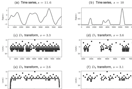
To illustrate the competing effects of support size and smoothness on the efficiency of the wavelet transformation, we simulate one-dimensional Gaussian random fields with Matérn covariances (same functionMand parametersband ν as in Eq. 2, but only one variable and one spatial dimen-sion). Figure A1 neatly demonstrates the concepts discussed
above: when the time series is uniformly smooth, the higher order waveletD4 delivers a far more efficient compression
thanD1(panels a, c, e). The situation changes when we
trun-cate the data (b, d, f): while D4 continues to be superior
within the smooth regions,D1, due to its shorter support,
re-quires fewer coefficients to represent the regions of constant zero values. This trade-off between representing smooth in-ternal structure and intermittency is precisely quantified by the entropy (defined in Eq. A1, values noted in the captions of Fig. A1), which measures the total degree of concentration on a small number of coefficients: while theD4does better in
both cases, the relative and absolute improvement is worse in the cut off case, where we introduced artificial singularities.
Figure A2 shows the results of our entropy-based wavelet-selection procedure for the model given by Eq. (1). We ob-serve that the model parameters have substantially more im-pact on the efficiency of the compression than the choice of wavelet. Fields with greater smoothness and larger scales (large values ofνand small values ofb) are represented far more compactly than rough small-scale cases, irrespective of the chosen basis. The differences between wavelets, while small in comparison, reveal a systematic behaviour: increas-ing support length leads to monotonously worse compression and the least asymmetric wavelets tend to fit slightly better than their “extremal phase” counterparts. The Haar wavelet constitutes an exception to this pattern, its entropy being fre-quently larger than that of several of its smoother cousins.
Besides theoretical optimality motivated by Eq. (3), prac-tical concerns can play an important role in the selection of an appropriate wavelet as well. Recalling that the bias-correction following Eckley et al. (2010) can introduce neg-ative values to the spectra, which have no intuitive interpre-tation, we are interested in seeing whether the problem can be circumvented by selecting an appropriate mother wavelet. Fig. A3 shows the ratio between negative and positive en-ergy in the mean spectra from the experiments discussed in Sect. 7.3. ForD1, this ratio is typically close to one-tenth.
Such large quantities of negative energy are rare forD2and
Figure A1.Realization of a one-dimensional Gaussian random vector with covarianceM(ν=3.5, b=2)(a)and the corresponding values of theD1transform and least asymmetricD4transform(c, e)which are greater than 0.1. Panels(b),(d), and(f)are the corresponding plots
for the cases where the vector is cut off at zero.
Competing interests. The authors declare that they have no conflict of interest.
Acknowledgements. We are very grateful to Rüdiger Hewer for pro-viding the original program code, as well as invaluable guidance for the stochastic rain model. Further thanks go to Franka Nawrath for providing efficient code to calculate the variogram score, as well as helpful discussions concerning its implementation. We would also like to thank Michael Weniger for many suggestions concerning the use of wavelets for forecast verification. Finally, our thanks go to Joseph Bellier and one anonymous reviewer for their constructive criticism and thoughtful suggestions.
Financial support. This research has been supported by the DFG (grant no. FR 2976/2-1).
Review statement. This paper was edited by Simon Unterstrasser and reviewed by Joseph Bellier and one anonymous referee.
References
Addison, P. S.: The illustrated wavelet transform handbook: in-troductory theory and applications in science, engineering, medicine and finance, CRC press, 2017.
Ahijevych, D., Gilleland, E., Brown, B. G., and Ebert, E. E.: Ap-plication of spatial verification methods to idealized and NWP-gridded precipitation forecasts, Weather Forecast., 24, 1485– 1497, 2009.
Bachmaier, M. and Backes, M.: Variogram or semivariogram? Vari-ance or semivariVari-ance? Allan variVari-ance or introducing a new term?, Math. Geosci., 43, 735–740, 2011.
Brune, S., Kapp, F., and Friederichs, P.: A wavelet-based analy-sis of convective organization in ICON large-eddy simulations, Q. J. Roy. Meteor. Soc., 144, 2812–2829, 2018.
Buschow, S.: wv_verif (Version 0.1.0), Zenodo, https://doi.org/10.5281/zenodo.3257511, 2019.
Casati, B., Ross, G., and Stephenson, D.: A new intensity-scale ap-proach for the verification of spatial precipitation forecasts, Me-teorol. Appl., 11, 141–154, 2004.
Cohen, A.: Numerical analysis of wavelet methods, vol. 32, Else-vier, 2003.
Daubechies, I.: Orthonormal bases of compactly supported wavelets, Commun. Pure Appl. Math., 41, 909–996, 1988.
A review and proposed framework, Meteorol. Appl., 15, 51–64, 2008.
Eckley, I. A., Nason, G. P., and Treloar, R. L.: Locally stationary wavelet fields with application to the modelling and analysis of image texture, J. Roy. Stat. Soc. C-Appl., 59, 595–616, 2010. Eckely, I. A. and Nason, G. P.: LS2W: Implementing the Locally
Stationary 2D Wavelet Process Approach in R, J. Stat. Softw., 43, 1–23, 2011.
Ekström, M.: Metrics to identify meaningful downscaling skill in WRF simulations of intense rainfall events, Environ. Model. Softw., 79, 267–284, 2016.
Gilleland, E.: Spatial forecast verification: Baddeley’s delta metric applied to the ICP test cases, Weather Forecast., 26, 409–415, 2011.
Gilleland, E., Ahijevych, D., Brown, B. G., Casati, B., and Ebert, E. E.: Intercomparison of spatial forecast verification methods, Weather Forecast., 24, 1416–1430, 2009.
Gilleland, E., Lindström, J., and Lindgren, F.: Analyzing the image warp forecast verification method on precipitation fields from the ICP, Weather Forecast., 25, 1249–1262, 2010.
Gneiting, T. and Raftery, A. E.: Strictly proper scoring rules, pre-diction, and estimation, J. Am. Stat. Assoc., 102, 359–378, 2007. Goel, P. K. and Vidakovic, B.: Wavelet transformations as diver-sity enhancers, Institute of Statistics & Decision Sciences, Duke University Durham, NC, 1995.
Haar, A.: Zur Theorie der orthogonalen Funktionensysteme, Math-ematische Annalen, 69, 331–371, 1910.
Han, F. and Szunyogh, I.: A Technique for the Verification of cipitation Forecasts and Its Application to a Problem of Pre-dictability, Mon. Weather Rev., 146, 1303–1318, 2018.
Hewer, R.: Stochastisch-physikalische Modelle für Windfelder und Niederschlagsextreme, PhD thesis, University of Bonn, available at: http://hss.ulb.uni-bonn.de/2018/5122/5122.htm (last access: 31 July 2019), 2018.
Hewer, R., Friederichs, P., Hense, A., and Schlather, M.: A Matérn-Based Multivariate Gaussian Random Process for a Consistent Model of the Horizontal Wind Components and Related Vari-ables, J. Atmos. Sci., 74, 3833–3845, 2017.
Kapp, F., Friederichs, P., Brune, S., and Weniger, M.: Spatial verifi-cation of high-resolution ensemble precipitation forecasts using local wavelet spectra, Meteorol. Z., 27, 467–480, 2018. Keil, C. and Craig, G. C.: A displacement and amplitude score
em-ploying an optical flow technique, Weather Forecast., 24, 1297– 1308, 2009.
Mallat, S.: A wavelet tour of signal processing, 3rd edition, Elsevier, Burlington MA, 294–296, 2009.
Marzban, C. and Sandgathe, S.: Verification with variograms, Weather Forecast., 24, 1102–1120, 2009.
Nason, G.: wavethresh: Wavelets Statistics and Transforms, avail-able at: https://CRAN.R-project.org/package=wavethresh (last access: 31 July 2019), r package version 4.6.8, 2016.
Nason, G. P., Von Sachs, R., and Kroisandt, G.: Wavelet processes and adaptive estimation of the evolutionary wavelet spectrum, J. Roy. Stat. Soc. B, 62, 271–292, 2000.
Radanovics, S., Vidal, J.-P., and Sauquet, E.: Spatial verification of ensemble precipitation: an ensemble version of SAL, Weather Forecast., 33, 1001–1020, 2018.
Roberts, N. M. and Lean, H. W.: Scale-selective verification of rain-fall accumulations from high-resolution forecasts of convective events, Mon. Weather Rev., 136, 78–97, 2008.
Rubner, Y., Tomasi, C., and Guibas, L. J.: The earth mover’s dis-tance as a metric for image retrieval, Int. J. Comput. Vision, 40, 99–121, 2000.
Scheuerer, M. and Hamill, T. M.: Variogram-based proper scor-ing rules for probabilistic forecasts of multivariate quantities, Mon. Weather Rev., 143, 1321–1334, 2015.
Schlather, M., Menck, P., Singleton, R., Pfaff, B., and R Core Team: RandomFields: Simulation and Analysis of Ran-dom Fields, available at: https://CRAN.R-project.org/package= RandomFields (last access: 31 July 2019), r package version 2.0.66, 2013.
Theis, S., Hense, A., and Damrath, U.: Probabilistic precipitation forecasts from a deterministic model: A pragmatic approach, Meteorol. Appl., 12, 257–268, 2005.
Thorarinsdottir, T. L., Gneiting, T., and Gissibl, N.: Using proper di-vergence functions to evaluate climate models, SIAM/ASA Jour-nal on Uncertainty Quantification, 1, 522–534, 2013.
Vidakovic, B. and Mueller, P.: Wavelets for kids, Instituto de Es-tadística, Universidad de Duke, 1994.
Villani, C.: Topics in Optimal Transportation, Graduate Studies in Mathematics, Volume 58, American Mathematical Society, Prov-idence, Rhode Island, 1st Edn., p. 75, 2003.
Weniger, M., Kapp, F., and Friederichs, P.: Spatial verification using wavelet transforms: A review, Q. J. Roy. Meteor. Soc., 143, 120– 136, 2017.