Disjoint Label Space Transfer Learning with Common Factorised Space

The Thirty-Third AAAI Conference on Artificial Intelligence (AAAI-19)

Disjoint Label Space Transfer Learning with Common Factorised Space

Xiaobin Chang,

Yongxin Yang,

Tao Xiang,

Timothy M. Hospedales

[email protected], [email protected], [email protected], [email protected]

Abstract

In this paper, a unified approach is presented to transfer learn-ing that addresses several source and target domain label-space and annotation assumptions with a single model. It is particularly effective in handling a challenging case, where source and target label-spaces aredisjoint, and outperforms alternatives in both unsupervised and semi-supervised set-tings. The key ingredient is a common representation termed

Common Factorised Space. It is shared between source and target domains, and trained with an unsupervised factorisa-tion loss and a graph-based loss. With a wide range of exper-iments, we demonstrate the flexibility, relevance and efficacy of our method, both in the challenging cases with disjoint la-bel spaces, and in the more conventional cases such as un-supervised domain adaptation, where the source and target domains share the same label-sets.

Introduction

Deep learning methods are now widely used in diverse ap-plications. However, their efficacy is largely contingent on a large amount of labelled data in the target task and do-main of interest. This issue continues to motivate intense in-terest in cross-task and cross-domain knowledge transfer. A wide range of transfer learning settings are considered which differ in whether the label spaces of source and target do-mains are overlapped (i.e., aligned or disjoint), as well as the amount of supervision/labelled training samples avail-able in the target domain (see Figure 1). The standard prac-tice offine-tuning(Yosinski et al. 2014) treats a pre-trained source model as a good initialisation for training a target problem model. It is adopted when the label spaces of both domains are either aligned or disjoint, but always requires a significant amount of labelled data from the target, albeit less than learning from scratch. Another popular problem is the unsupervised domain adaptation (UDA), where knowl-edge is transferred from a labelled source domain to an un-labelled target domain (Tzeng et al. 2017; Ganin et al. 2016; Cao, Long, and Wang 2018). UDA makes the simplifying assumption that the label space of source and target do-mains are the same, and focuses on narrowing the distri-bution gap between source and target domains without any labelled samples from the target.

Copyright c2019, Association for the Advancement of Artificial Intelligence (www.aaai.org). All rights reserved.

Supervised Unsupervised Semi-supervised

Disjoint Aligned

So

u

rce

&

T

ar

g

et

L

ab

el

Sp

ace

Target Supervision

Semi-supervised DLSTL Unsupervised

DLSTL Unsupervised

Domain Adaptation Fine-tuning

Fine-tuning

Figure 1: Schematic of various transfer learning problems on two criteria: the relation between source and target label space, and the amount of target problem supervision.

Wang et al. 2018). Source and target data can be aligned within the attribute space, in order to alleviate the impacts of disjoint label space in DLSTL problems. Nevertheless, attribute can be expensive to acquire which prevents it form being widely applicable.

In this paper, a novel transfer learning model is pro-posed, which focuses on handling the most challenging set-ting,unsupervised DLSTLbut is applicable to other settings including semi-supervised DLSTL and UDA. The model, termed common factorised space model (CFSM), is devel-oped based on the simple idea that recognition should be performable in a shared latent factor space for both do-mains where each factor can be interpreted as latent attribute (Fu et al. 2014; Rastegari, Farhadi, and Forsyth 2012). In order to automatically discover such discriminative latent factors and align them for transferring knowledge across datasets/domains, our inductive bias is that input samples from both domains should generate low-entropy codes in this common space, i.e., near binary-codes (Salakhutdinov and Hinton 2009; Zhu et al. 2016). This is a weaker assump-tion than distribuassump-tion matching, but does provide a criterion that can be optimised to align the two domains in the absence of common label space and/or labelled target domain train-ing samples. Specifically, both domains should be explain-able in terms of the same set of discriminative latent factors with high certainty. As a result, discriminative information from the source domain can be more effectively transferred to the target through this common factorised space. To im-plement this model in a neural network architecture, a com-mon factorised space (CFS) layer is inserted between the feature output layer (the penultimate layer) and the classi-fication layer (the final layer). This layer is shared between both domains and thus forms a common space. An unsuper-vised factorisation loss is then derived and applied on such common space which serves the purpose of optimising low-entropy criterion for discriminative latent factors discovery.

Somewhat uniquely, cross-domain knowledge transfer of the proposed CFSM occurs at a relatively high layer (i.e., CFS layer). Particularly when the target domain problem is a retrieval one, it is important that this knowledge is prop-agated down from CFS to feature extraction for effective knowledge transfer. To assist this process we define a novel graph Laplacian-based loss - which builds a graph in the higher-level CFS, and regularises the lower-level network feature output to have matching similarity structure. i.e., that inter-sample similarity structure in the shared latent factor space should be reflected in earlier feature extraction. This top-down regularisation is opposite to the use of Laplacian regularisation in existing works (Belkin, Niyogi, and Sind-hwani 2006; Yang et al. 2017) which are bottom-up, i.e., graph from lower-level regularises the higher-level features. This unique design is due to the fact that, although both spaces (CFS and feature) are latent, the former is closer to supervisions (e.g., from the labelled source data) and more aligned thanks to the factorisation loss, and thus more dis-criminative and ‘trustworthy’.

Contributions of the paper are as follows: 1. A unified ap-proach to transfer learning is proposed. It can be applied to different transfer learning settings but is particularly

at-tractive in handling the most challenging setting of unsu-pervised DLSTL. This setting is under-studied with the lat-est efforts focus on the easier semi-supervised DLSTL set-ting (Luo et al. 2017) with partially labelled target data. Sev-eral topical applications in computer vision such as person re-identification (Re-ID) and sketch-based image retrieval (SBIR) can be interpreted as unsupervised DLSTL which reveals its vital research and application values. 2. We pro-pose a deep neural network based model, called common factorised space model (CFSM), that provides the first sim-ple yet effective method for unsupervised DLSTL; it can be easily extended to semi-supervised DLSTL as well as conventional UDA problems. 3. A novel graph Laplacian-based loss is proposed to better exploit the more aligned and discriminative supervision from higher-level to improve deep feature learning. Finally, comprehensive experiments on various transfer learning settings, from UDA to DLSTL, are conducted. CFSM achieves state-of-the-art results on both unsupervised and semi-supervised DLSTL problems and performs competitively in standard UDA. The effective-ness and flexibility of the proposed model on transfer learn-ing problems are thus demonstrated.

Related Work

Transfer Learning

Transfer learning (TL) aims to transfer knowledge from one domain/task to improve performance on the another (Pan, Yang, and others 2010). The most widely used TL tech-nique for deep networks is fine-tuning (Yosinski et al. 2014; Chen et al. 2018; Ren et al. 2015). Instead of training a target network from scratch, its weights are initialised by a pre-trained model from another task such as ImageNet (Deng et al. 2009) classification. While fine-tuning reduces label requirement compared to learning the target problem from scratch, it is prone to over-fitting if target labels are very few (Yosinski et al. 2014). Therefore, it is ineffective for very sparsely supervised DLSTL, and not applicable to unsuper-vised DLSTL. Moreover, vanilla TL does not exploit avail-able unlabelled samples for the target problem (i.e. semi-supervised TL). The most related method to ours is (Luo et al. 2017) which does exploit both unlabelled and few labelled data, i.e., semi-supervised DLSTL. However like other TL methods, it does not generalise to the unsupervised DLSTL setting where no target annotations are available.

UDA by allowing target domain to have some novel cate-gories in addtion to the shared ones. It focuses on identifying shared categories and aligning those. DLSTL is a more gen-eral problem setting than OSDA, since there is no assump-tion of any shared categories. Related to our approach that exploits a common factorisation space to discover shared la-tent factors/attributes, semantic attributes have been used to improve domain adaptation performance (Su et al. 2016), for example by enabling new types of self-training (Chen et al. 2015; Wang et al. 2018) and consistency losses (Ge-bru, Hoffman, and Li 2017). However these methods require the attribute definition and annotation, at least in the source domain. In contrast, no expensive attribute annotation is re-quired in our model.

Deep Binary Representation Learning

The use of binary codes for hashing with deep networks goes back to (Salakhutdinov and Hinton 2009). In computer vision, hashing layers were inserted between feature- and classification-layers to provide a hashing code (Lin et al. 2015; Zhu et al. 2016). To produce a binary representation for fast retrieval, a threshold is applied on the sigmoid acti-vated hashing layer (Lin et al. 2015). Our method is similar in working with a near-binary penultimate layer. However there are several key differences: First, our CFS serves a very different purpose to a hash code. We focus on TL to a new domain with new label-space, and the role of our CFS is to provide a representation with which different domains can be more aligned for knowledge transfer, rather than for effi-cient retrieval. In contrast, existing hashing methods follow the conventional supervised learning paradigm within a sin-gle domain. Second, the proposed CFS is only near-binary due to a low-entropy loss, rather than sacrificing representa-tion power for an exactly binary code.

Semi-supervised Learning

Graph-based regularisation is popular for semi-supervised learning (SSL) which uses both labelled and unlabelled data to achieve better performance than learning with la-belled data only (Zhu 2006; Belkin, Niyogi, and Sindhwani 2006). In SSL, graph based regularisation is applied to regu-larise model predictions to respect the feature-space man-ifold (Yue et al. 2017; Nadler, Srebro, and Zhou 2009; Belkin, Niyogi, and Sindhwani 2006). Moreover, exploiting the graph from lower-level to regularise higher-level fea-tures is widely adopted in other scenarios, e.g., unsuper-vised learning (Jia et al. 2015; Yang et al. 2017). Due to the source→target knowledge transfer, the more ‘trustwor-thy’ layer in our method is the penultimate CFS layer, as it is closer to the supervision, rather than the feature space layer. Therefore our regularisation is applied to encourage the feature-extractor to learn representations that respect the CFS manifold shared by both domains, i.e., the regularisa-tion direcregularisa-tion is opposite to that in existing models.

Entropy loss for unlabelled data is another widely used SSL regulariser (Zhu 2006; Long et al. 2016). It is applied at the classification layer in problems where the unlabelled and labelled data share the same label-space – and reflects the inductive bias that a classification boundary should not

cut through the dense unlabelled data regions. Its typical use is on softmax classifier outputs where it encourages a classi-fier to pick a single label. In contrast we use entropy-loss to solve DLSTL problems by applying it element-wise on our intermediate CFS layer in order to weakly align domains by encouraging them to share a near-binary representation.

Methodology

Definition and notation For Disjoint Label Space Trans-fer Learning (DLSTL), there is a source (labelled) domain

S and a target (unlabelled or partially labelled) domain

T1_{. The key characteristic of DLSTL is the disjoint label} space assumption, i.e., the source YS and targetYT label

spaces are potentially disjoint: YS ∩ YT = ∅. Instances

from source/target domains are denotedXSandXT

respec-tively. The combined inputs{XS, XT}are denoted asX. To

present our model, we stick mainly to the most challenging unsupervised DLSTL setting where target labels are totally absent. The easier cases, e.g., semi-supervised DLSTL and UDA, can then be handled with minor modifications.

Model Architecture

The proposed model architecture consists of three modules, a feature extractorF = ΦθM(X)that can be any deep neural

network and is shared between all domains. This is followed by a fully connected layer and sigmoid activationσ, which define the Common Factorised Space (CFS) layer. This pro-vides a representation of dimensiondC,FC = ΨθC(·) =

σ(WΦθM(·) +b). Recall that the goal of CFS is to learn

a latent factor (low-entropy) representation for both source and target domains. The sigmoid activation means that the layer’s scale is FC ∈ (0,1)dC_{, so activations near 0 or 1}

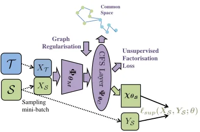
can be interpreted as the corresponding latent factor being present or absent. To encourage a near-binary representa-tion, unsupervised factorisation loss is applied. For the la-belled source domain only, the pre-activated FC are then classified by softmax classifierχθ_S with cross-entropy loss. The overall architecture is illustrated in Figure 2.

Regularised Model Optimisation

The parameters of the proposed CFSM are θ := {θM, θC, θS}including parameters of the feature extractor θM, CFS layerθCand source classifierθS. The training pro-cedure can be formulated as a maximum-a-posterior (MAP) learning given labelled source{XS, YS}and unlabelled

tar-get dataXT,

ˆ

θ= argmax

θ

p(θ|XS, YS, XT), (1)

wherep(θ|XS, YS, XT)is the posterior of model parameter

θgiven dataXS, YS, XT. This can be rewritten as

p(θ|XS, YS, XT)∝p(θ, XS, YS, XT)

∝p(YS|XS, XT, θ)p(θ|XS, XT).

(2)

So the optimisation in Eq. 1 is equivalently

ˆ

θ= argmax

θ

p(YS|XS, θ)p(θ|X). (3)

1

Sampling mini-batch

Common Space

Graph Regularisation

Unsupervised Factorisation Loss

Figure 2: The proposed model architecture is illustrated. Dif-ferent colours corresponding to difDif-ferent data streams. Green indicates source data. Blue is used for target data. Purple means joint data from both source and target domains.

The first term p(YS|XS, θ) in Eq. 3 represents the

likeli-hood of source labels w.r.t. θ. Optimising this term is a conventional supervised learning task with a loss denoted `sup(XS, YS;θ).

The second termp(θ|X)in Eq. 3 is a prior depending on the input dataXof both source and target datasets. From an optimisation perspective, this is the regulariser that will play the key role in solving unsupervised DLSTL problems since it requires no labels. Given the model architecture, it can be further decomposed as:

p(θ|X) =p(θM, θC|X)

=p(θC|θM, X)p(θM|X), (4)

whereθS is excluded since no supervision is used.

Specifi-cally, the first termp(θC|θM, X)serves as the regulariser on the CFS layer while the second termp(θM|X)regularises the deep feature extractorΦθM.

Low-Entropy Regularisation: Unsupervised Adaptation We first discuss how to define the priorp(θC|θM, X) regu-lariser for CFS layer. The sigmoid activated outputsFCfrom CFS layerΨθC can be interpreted as multi-label predictions

on latent factors. The uncertainty measure for label predic-tion can be defined by using its entropy

h(θC|θM, X) =− N

X

i=1

< FC,i,log(FC,i)>

=−

N

X

i=1

<ΨθC(xi),log(ΨθC(xi))>

(5)

where FC,i denotes the common factor representation

ΨθC(xi) of instance xi ∈ X. This is applied on both

source and target data, soN is the number of instances in both datasets.log(·)is applied element-wise, and<·, · > is vector inner product. According to the low-uncertainty criterion (Carlucci et al. 2017), optimising the prior term p(θC|θM, X) can be achieved by minimising this uncer-tainty measure. Eq. 5 is thus the regulariser corresponding

to the prior p(θC|θM, X). Specifically, this loss biases the representationFCto contain more certain predictions, e.g., closer to 0 or 1 for each discovered latent factor. Therefore, we denote it as unsupervised factorisation loss.

In summary, the low-entropy regulariser on CFS is built upon the assumption that the two domains share a set of la-tent attributes and that if a source classifier is well adapted to the target, then the presence/absence of these attributes should be certain for each instance. Therefore, it essentially generalises the low-uncertainty principle (widely used in ex-isting unsupervised and semi-supervised learning literature) to the disjoint label space setting.

Graph Regularisation: Robust Feature Learning The second prior in Eq. 4 isp(θM|X)which acts as the regu-lariser for the feature extractorΦθM. The unique property of

our setup so far is that the knowledge transfer into the target domain is via the CFS layer; therefore we are interested in ensuring that the feature extractor network extracts features whose similarity structure reflects that of the latent factors in the CFS layer. Unlike conventional graph Laplacian losses that regularise higher-level features with a graph built on lower-level features (Belkin, Niyogi, and Sindhwani 2006; Zhu 2006), we do the reverse and regularise the feature ex-tractorΦθM to reflect the similarity structure inFC. This is

particularly important for applications where the target prob-lem is retrieval, because we use deep featuresF = ΦθM(·)

as an image representation.

The proposed graph loss is expressed as

Tr(FT∆FCF), (6)

where∆FC is the graph Laplacian (Cai et al. 2011) built on

the common space featuresFC.

Summary We unify the proposed model architecture θ := {θM, θC, θDS} with source {XS, YS} and target

{XT} data for unsupervised DLSTL problems from an

maximum-a-posterior (MAP) perspective. This decomposes into a standard supervised term p(YS|XS, θ)(source data

only) and data-driven priors for the CFS layer and fea-ture extraction module. They correspond to supervised loss `sup(XS, YS;θ), unsupervised factorisation loss (Eq. 5) and

the graph loss (Eq. 6) respectively. Taking all terms into ac-count, the final optimisation objective of Eq. 3 is

L(θ) =`sup(XS, YS;θ) +βMT r(FT∆FCF)

−βC 1

N N

X

i=1

< FC,i,log(FC,i)> . (7)

whereβCandβM are balancing hyper-parameters. In order to select βC and βM, the model is first run by setting all weights to 1; after the first few iterations, we check the val-ues of each loss. We then set the two hyper-parameters to rescale the losses to a similar range so that all three terms contribute approximately equally to the training.

scheduling: each mini-batch contains samples from both source and target domains. The supervised loss is applied only to source samples with corresponding supervision, the entropy and graph losses are applied to both, and the graph is built per-mini-batch. In this work, the number of source and target samples are equally balanced in a mini-batch.

Experiments

The proposed model is evaluated on progressively more challenging problems. First, we evaluate CFSM on unsuper-vised domain adaptation (UDA). Second, different DLSTL settings are considered, including semi-supervised DLSTL classification and unsupervised DLSTL retrieval. CFSM handles all these scenarios with minor modifications. The effectiveness CFSM is demonstrated by its superior perfor-mance compared to the existing work. Finally insight is pro-vided through ablation study and visualisation analysis.

Unsupervised Domain Adaptation: SVHN-MNIST

Dataset and Settings We evaluate the UDA setting from (Ganin et al. 2016) where SVHN (Netzer et al. 2011) is the labelled source dataset and MNIST (LeCun et al. 1998) is the unlabelled target. For fair comparison we use an identi-cal feature extractor network to (Luo et al. 2017). Our CFSM is pre-trained on the source dataset with cross-entropy su-pervision anddC= 50, followed by joint training on source and target with our regularisers as in Eq. 7. Since the label-space is shared in UDA, we also apply entropy loss on the softmax classification of the target (Long et al. 2016). We setβM = 0.001andβC= 0.01.

Results We compare our method with two baselines. Source only: Supervised training on the source and directly apply to target data. Joint FT: Model is initialised with source pre-train, and fine-tuning on both domains with su-pervised loss for source and semi-susu-pervised entropy loss for target. We also compare several deep UDA methods including Gradient Reversal (Ganin et al. 2016), Domain Confusion (Tzeng et al. 2015), ADDA (Tzeng et al. 2017), Label Efficient Transfer (LET) (Luo et al. 2017), Asym. tri-training (Saito, Ushiku, and Harada 2017) and Res-para (Rozantsev, Salzmann, and Fua 2018).

As shown in Table 1, CFSM boosts the performance on both baselines with clear margin (25.5% and9.3% vs. Source only and Joint FT respectively). Moreover, it is5.5%

higher than LET (Luo et al. 2017), the nearest competitor and only alternative thatalsoaddresses the DLSTL setting.

Semi-supervised DLSTL: Digit Recognition

Dataset and Settings We follow the semi-supervised DL-STL recognition experiment of (Luo et al. 2017) where again two digit datasets, SVHN and MNIST, are used. Images of digits 0 to 4 from SVHN are fully labelled as source data while images of digits 5 to 9 from MNIST are target data. The target dataset has sparse labels (klabels per class) and unlabelled images available. Thus we also add a classifier χθT after the CFS layerΨθC for the target categories.

The feature extractor architectureΦθMis exactly the same

as in (Luo et al. 2017) for fair comparison. We pre-train

Method Accuracy

Domain confusion ICCV’15 68.1 Grad. reversal JMLR’16 73.9 ADDA CVPR’17 76.0

LET NIPS’17 81.0

Res-para CVPR’18 84.7 Asym. tri-training ICML’17 85.0

Source only 61.0

Joint FT 77.2

CFSM 86.5

Table 1: Unsupervised domain adaptation results. Classifi-cation accuracy (%) on SVHN→MNIST transfer.

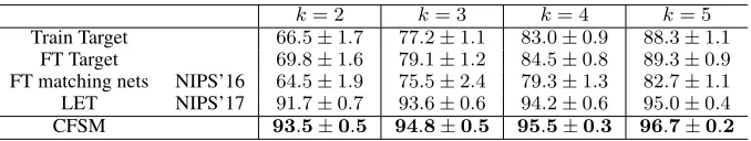
CFSM on source data as initialisation, and then train it with both source and target data using only loss in Eq. 7. We set dC = 10, βM =βC = 0.01. The learning rate is0.001and the Adam (Kingma and Ba 2014) optimiser is used. Results The results for several degrees of target label sparsity k = 2,3,4,5 (corresponding to 10,15,20,25 la-belled samples, or0.034%,0.050%,0.066%,0.086%of to-tal target training data respectively), are reported in Table 2. Results are averaged over ten random splits as in (Luo et al. 2017). Besides the FT matching nets (Vinyals et al. 2016) and state-of-the-art LET results from (Luo et al. 2017), we run two baselines: Train Target: Training CFSM architecture from scratch with partially labelled target data only, and FT Target: The standard train/fine-tune pipeline, i.e., pre-train on the labelled source, and fine-tune on the labelled target samples only.

As shown in Table 2, the performances of baseline models are significantly lower than LET and the proposed CFSM. The Train Target baseline performs poorly as it is hard to achieve good performance with few target samples and no knowledge transfer from source. The Fine-Tune Target base-line performs poorly as the annotation here is too sparse for effective fine-tuning on the target problem. Fine-Tune matching nets follows the5-way(k−1)-shot learning with sparsely labelled target data only, but no improvement is shown over the other baselines. Our proposed CFSM consis-tently outperforms the state-of-the-art LET alternative. For example, under the most challenging setting (k= 2), CFSM is1.8%higher than LET on mean accuracy and0.2%lower on standard error.

Unsupervised DLSTL: ReID and SBIR

k= 2 k= 3 k= 4 k= 5

Train Target 66.5±1.7 77.2±1.1 83.0±0.9 88.3±1.1

FT Target 69.8±1.6 79.1±1.2 84.5±0.8 89.3±0.9

FT matching nets NIPS’16 64.5±1.9 75.5±2.4 79.3±1.3 82.7±1.1

LET NIPS’17 91.7±0.7 93.6±0.6 94.2±0.6 95.0±0.4

CFSM 93.5±0.5 94.8±0.5 95.5±0.3 96.7±0.2

Table 2: Semi-supervised DLSTL image categorisation results (%), with mean classification accuracy and standard error for SVHN (0-4)→MNIST (5-9).

M2D D2M

model R1 mAP R1 mAP

UMDL CVPR’16 18.5 7.3 34.5 12.4 PTGAN CVPR’18 27.4 - 38.6 -PUL arXiv’17 30.0 16.4 45.5 20.5 CAMEL ICCV’17 - - 54.5 26.3 TJ-AIDL CVPR’18 44.3 23.0 58.2 26.5 SPGAN CVPR’18 46.4 26.2 57.7 26.7 MMFA BMVC’18 45.3 24.7 56.7 27.4 CFSM 49.8 27.3 61.2 28.3

Table 3: Unsupervised transfer for person Re-ID (%). M2D indicates Market as source dataset and Duke as target, vice versa. Target Dataset Performance is reported.

for unsupervised person Re-ID: Market (Zheng et al. 2015) and Duke (Zheng, Zheng, and Yang 2017). ImageNet pre-trained Resnet50 (He et al. 2016) is used as the feature ex-tractor ΦθM. Cross-entropy loss with label smoothing and

triplet loss are used for the source domain as supervised learning objectives. We setdC = 2048, βM = 2.0, βC =

0.01. Adam optimiser is used with learning rate3.5e−4. We treat each dataset in turn as source/target and perform unsu-pervised transfer from one to the other. Rank 1 (R1) accu-racy and mean Average Precision (mAP) results on the target datasets are used as evaluation metrics.

In Table 3, We show that our method outperforms the state-of-the-art alternatives purpose-designed for unsu-pervised person Re-ID: UMDL (Peng et al. 2016), PT-GAN (Wei et al. 2018), PUL (Fan, Zheng, and Yang 2017), CAMEL (Yu, Wu, and Zheng 2017), TJ-AIDL (Wang et al. 2018), SPGAN (Deng et al. 2018) and MMFA (Lin et al. 2018). Note that TJ-AIDL and MMFA exploit attribute la-bels to help alignment and adaptation. The proposed method automatically discovers latent factors with no additional an-notation. However, CFSM improves at least3.0%over TJ-AIDL and MMFA on the R1 accuracy of both settings.

FG-SBIR Fine-grained Sketch Based Image Retrieval (SBIR) focuses on matching a sketch with its corresponding photo (Sangkloy et al. 2016). As demonstrated in (Sangkloy et al. 2016), object category labels play an important role in retrieval performance, so existing studies make a closed world assumption, i.e., all testing categories overlap with training categories. However, if deploying SBIR in a real application such as e-commerce (Yu et al. 2016), one would like to train the SBIR system once on some source object categories, and then deploy it to provide sketch-based im-age retrieval of new categories without annotating new data

and re-training for the target object category. Unsupervised adaptation to new categories without sketch-photo pairing labels is therefore another example of the unsupervised DL-STL problem. Comparing to Re-ID, where instances are per-son images in different camera views, instances in SBIR are either photos or hand-drawn sketches of objects.

There are 125 object classes in the Sketchy dataset (Sangkloy et al. 2016). We randomly split 75

classes as a labelled source domain and use the remaining

50 classes to define an unlabelled target domain with disjoint label space. ImageNet pre-trained Inception-V3 (Szegedy et al. 2016) is used as the feature extractor

ΦθM. Cross-entropy and triplet loss are used for source

supervision. We set dC = 512, βM = 10−3, βC = 0.1. Adam optimiser with learning rate 10−4 is used. As a baseline, Source Only is the direct transfer alternative that uses the same architecture but trains on the source labelled data only, and is applied directly to the target without adaptation. The retrieval performance on unseen classes (tar. cls.) are reported. Results are averaged over10random splits. As shown in Table 4, the proposed CFSM improves the retrieval accuracy on unseen cases by2.48%.

Source only CFSM tar. cls. 23.74±0.24 26.22±0.25

Table 4: SBIR: Sketch-photo retrieval results (%). Averaged Rank 1 accuracy and standard error.

Further Analysis

Ablation study Unsupervised person Re-ID is chosen as the main benchmark for an ablation study. Firstly because it is a challenging and realistic large-scale problem in the un-supervised DLSTL setting, and secondly because it provides a bidirectional evaluation for more comprehensive analysis. The following ablated variants are proposed and com-pared with the full CFSM. Source Only: The proposed ar-chitecture is learned with source data and supervised losses only. Source+Regs: The regularisers, unsupervised factori-sation and graph losses can be added with source dataset only. CFSM−Graph: Our method without the proposed graph loss. CFSM+ClassicGraph: Replacing our proposed graph loss with a conventional Laplacian graph (i.e., graphs constructed in lower-level feature space extracted byΦθMto

M2D D2M model R1 mAP R1 mAP Source Only 39.2 20.2 54.4 23.0 Source+Regs 41.6 21.2 55.8 24.0 AE 43.6 22.8 56.4 24.9 CFSM−Graph 46.8 25.6 60.0 27.6 CFSM+ClassicGraph 47.4 26.1 59.0 27.0 CFSM 49.8 27.3 61.2 28.3

Table 5: Ablation study on unsupervised person Re-ID benchmarks. Target dataset performance (%) is reported.

In this case both source and target data are used and the re-construction error provides the regularisation loss.

The results are shown in Table 5. Firstly, by compar-ing the variants that use source data only (Source Only and Source+Regs) with the joint training methods, we find they are consistently inferior. This illustrates that it is cru-cial to leverage target domain data for adaptation. Sec-ondly, CFSM and its variants consistently achieve bet-ter results than AE, illustrating that our unsupervised fac-torisation loss and graph losses provide better regulari-sation for cross-domain/cross-task adaptation. The effec-tiveness of our graph loss is illustrated by two com-parisons: (1) CFSM−Graph is worse than CFSM, show-ing the contribution of the graph loss; and (2) replac-ing our graph loss with the conventional Laplacian graph loss (CFSM+ClassicGraph) shows worse results than ours, justifying our choice of regularisation direction. Finally, we note that applying our regularisers to the source only (Source+Regs) still improves the performance slightly on target dataset vs Source Only. This shows that training with these regularisers has a small benefit to representation trans-ferability even without adaptation.

Visualisation analysis To understand the impact of unsu-pervised factorisation loss, Figure 3 illustrates the distribu-tion of target CFS activadistribu-tions in the semi-supervised DLSTL setting (SVHN→MNIST). The left plot shows the activa-tions without any such loss, leading to a distribution of mod-erate predictions peaked around 0.5. In contrast, the right plot shows the activation distribution on the target dataset of CFSM. We can see that our regulariser has indeed induced the target dataset to represent images with a low–entropy near-binary code. We also compare training a source model by adding low-entropy CFS loss, and then applying it to the target data. This leads to a low-entropy representation of the source data, but the middle plot shows that when trans-ferred to the target dataset or adaptation the representation becomes high-entropy. That is, joint training with our losses is crucial to drive the adaptation that allows target dataset to be represented with near-binary latent factor codes.

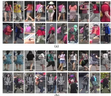
Qualitative Analysis We visualise the discovered latent attributes qualitatively. For each element in FC, we rank images in both source and target domains by their activa-tion. Person images corresponding to the highest ten values of a specific FC are recorded. Figure 4 shows two exam-ple factors with images from the source (first row) and tar-get (second row) dataset. We can see that the first example in Figure 4(a) is a latent attribute for the colour ‘red’

cov-Src. pre-trained

0 0.5 1

0 200 600

1000 Src. entropy FT

0 0.5 1

0 200 600

1000 Unsup. factor. loss

0 0.5 1

0 500 1000 1500

Figure 3: CFS activations distribution on target data. Left: Train on source with supervised loss. Middle: Train on source with both supervised and low-entropy CFS losses. Right: CFSM, jointly trained on source and target.

(a)

(b)

Figure 4: Illustration of images selected by two different la-tent factors: (a) red and (b) female/textured/bag-carrying. In each case the top row is the source (Market) data and the bottom row is the target (Duke) data. Best viewed in colour.

ering both people’s bags and clothes. The second example in Figure 4(b) is a higher-level latent attribute that is selec-tive for both females, as well as textured clothes and bag-carrying. Importantly, these factors have become selective for the same latent factors across datasets, although the tar-get dataset has no supervision (i.e., unsupervised DLSTL).

Conclusion

We studied a challenging transfer learning setting DLSTL, where the label space between source and target labels are disjoint, and the target dataset has few or no labels. In order to transfer the discriminative cues from the labelled source to the target, we propose a simple yet effective model which uses an unsupervised factorisation loss to discover a com-mon set of discriminative latent factors between source and target datasets. And to improve feature learning for subse-quent tasks such as retrieval, a novel graph-based loss is fur-ther proposed. Our method is both the first solution to the unsupervised DLSTL, and also uniquely provides a single framework that is effective at both unsupervised and semi-supervised DLSTL as well as the standard UDA.

References

Belkin, M.; Niyogi, P.; and Sindhwani, V. 2006. Manifold regu-larization: A geometric framework for learning from labeled and unlabeled examples.JMLR.

Busto, P. P., and Gall, J. 2017. Open set domain adaptation. In

ICCV.

Cai, D.; He, X.; Han, J.; and Huang, T. S. 2011. Graph regularized nonnegative matrix factorization for data representation.TPAMI. Cao, Y.; Long, M.; and Wang, J. 2018. Unsupervised domain adaptation with distribution matching machines.AAAI.

Carlucci, F. M.; Porzi, L.; Caputo, B.; Ricci, E.; and Bul`o, S. R. 2017. Autodial: Automatic domain alignment layers.ICCV. Chen, Q.; Huang, J.; Feris, R.; Brown, L. M.; Dong, J.; and Yan, S. 2015. Deep domain adaptation for describing people based on fine-grained clothing attributes.CVPR.

Chen, H.; Wang, Y.; Wang, G.; and Qiao, Y. 2018. Lstd: A low-shot transfer detector for object detection.arXiv.

Deng, J.; Dong, W.; Socher, R.; Li, L.-J.; Li, K.; and Fei-Fei, L. 2009. Imagenet: A large-scale hierarchical image database.CVPR. Deng, W.; Zheng, L.; Kang, G.; Yang, Y.; Ye, Q.; and Jiao, J. 2018. Image-image domain adaptation with preserved self-similarity and domain-dissimilarity for person re-identification.CVPR.

Fan, H.; Zheng, L.; and Yang, Y. 2017. Unsupervised person re-identification: Clustering and fine-tuning.arXiv.

Fu, Y.; Hospedales, T.; Xiang, T.; and Gong, S. 2014. Learning multi-modal latent attributes.TPAMI.

Ganin, Y.; Ustinova, E.; Ajakan, H.; Germain, P.; Larochelle, H.; Laviolette, F.; Marchand, M.; and Lempitsky, V. 2016. Domain-adversarial training of neural networks.JMLR.

Gebru, T.; Hoffman, J.; and Li, F.-F. 2017. Fine-grained recogni-tion in the wild: A multi-task domain adaptarecogni-tion approach.ICCV. He, K.; Zhang, X.; Ren, S.; and Sun, J. 2016. Deep residual learn-ing for image recognition.CVPR.

Jia, K.; Sun, L.; Gao, S.; Song, Z.; and Shi, B. E. 2015. Lapla-cian auto-encoders: an explicit learning of nonlinear data manifold.

Neurocomputing.

Kingma, D. P., and Ba, J. 2014. Adam: A method for stochastic optimization.arXiv.

LeCun, Y.; Bottou, L.; Bengio, Y.; and Haffner, P. 1998. Gradient-based learning applied to document recognition. IEEE Proceed-ings.

Lin, K.; Yang, H.-F.; Hsiao, J.-H.; and Chen, C.-S. 2015. Deep learning of binary hash codes for fast image retrieval.CVPRW. Lin, S.; Li, H.; Li, C.-T.; and Kot, A. C. 2018. Multi-task mid-level feature alignment network for unsupervised cross-dataset person re-identification.BMVC.

Long, M.; Zhu, H.; Wang, J.; and Jordan, M. I. 2016. Unsupervised domain adaptation with residual transfer networks.NIPS. Luo, Z.; Zou, Y.; Hoffman, J.; and Fei-Fei, L. F. 2017. Label ef-ficient learning of transferable representations across domains and tasks.NIPS.

Nadler, B.; Srebro, N.; and Zhou, X. 2009. Semi-supervised learn-ing with the graph laplacian: The limit of infinite unlabelled data.

NIPS.

Netzer, Y.; Wang, T.; Coates, A.; Bissacco, A.; Wu, B.; and Ng, A. Y. 2011. Reading digits in natural images with unsupervised feature learning.NIPSW.

Pan, S. J.; Yang, Q.; et al. 2010. A survey on transfer learning.

TKDE.

Peng, P.; Xiang, T.; Wang, Y.; Pontil, M.; Gong, S.; Huang, T.; and Tian, Y. 2016. Unsupervised cross-dataset transfer learning for person re-identification. CVPR.

Rastegari, M.; Farhadi, A.; and Forsyth, D. 2012. Attribute discov-ery via predictable discriminative binary codes.ECCV.

Rebuffi, S.-A.; Bilen, H.; and Vedaldi, A. 2017. Learning multiple visual domains with residual adapters.NIPS.

Ren, S.; He, K.; Girshick, R.; and Sun, J. 2015. Faster r-cnn: Towards real-time object detection with region proposal networks.

NIPS.

Rozantsev, A.; Salzmann, M.; and Fua, P. 2018. Residual parame-ter transfer for deep domain adaptation.CVPR.

Saito, K.; Ushiku, Y.; and Harada, T. 2017. Asymmetric tri-training for unsupervised domain adaptation. ICML.

Salakhutdinov, R., and Hinton, G. 2009. Semantic hashing. Inter-national Journal of Approximate Reasoning.

Sangkloy, P.; Burnell, N.; Ham, C.; and Hays, J. 2016. The sketchy database: Learning to retrieve badly drawn bunnies.SIGGRAPH. Su, C.; Zhang, S.; Xing, J.; Gao, W.; and Tian, Q. 2016. Deep attributes driven multi-camera person re-identification.ECCV. Sun, B., and Saenko, K. 2016. Deep coral: Correlation alignment for deep domain adaptation.ECCVW.

Szegedy, C.; Vanhoucke, V.; Ioffe, S.; Shlens, J.; and Wojna, Z. 2016. Rethinking the inception architecture for computer vision.

CVPR.

Tzeng, E.; Hoffman, J.; Darrell, T.; and Saenko, K. 2015. Simul-taneous deep transfer across domains and tasks.ICCV.

Tzeng, E.; Hoffman, J.; Saenko, K.; and Darrell, T. 2017. Adver-sarial discriminative domain adaptation.CVPR.

Vinyals, O.; Blundell, C.; Lillicrap, T.; Wierstra, D.; et al. 2016. Matching networks for one shot learning. NIPS.

Wang, J.; Zhu, X.; Gong, S.; and Li, W. 2018. Transferable joint attribute-identity deep learning for unsupervised person re-identification.CVPR.

Wei, L.; Zhang, S.; Gao, W.; and Tian, Q. 2018. Person transfer gan to bridge domain gap for person re-identification.CVPR. Yang, S.; Li, L.; Wang, S.; Zhang, W.; and Huang, Q. 2017. A graph regularized deep neural network for unsupervised image rep-resentation learning.CVPR.

Yosinski, J.; Clune, J.; Bengio, Y.; and Lipson, H. 2014. How transferable are features in deep neural networks?NIPS.

Yu, Q.; Liu, F.; Song, Y.-Z.; Xiang, T.; Hospedales, T. M.; and Loy, C. C. 2016. Sketch me that shoe.CVPR.

Yu, H.-X.; Wu, A.; and Zheng, W.-S. 2017. Cross-view asymmetric metric learning for unsupervised person re-identification.ICCV. Yue, Z.; Meng, D.; He, J.; and Zhang, G. 2017. Semi-supervised learning through adaptive laplacian graph trimming. Image and Vision Computing.

Zheng, L.; Shen, L.; Tian, L.; Wang, S.; Wang, J.; and Tian, Q. 2015. Scalable person re-identification: A benchmark. ICCV. Zheng, Z.; Zheng, L.; and Yang, Y. 2017. Unlabeled samples gen-erated by gan improve the person re-identification baseline in vitro.

ICCV.

Zhu, H.; Long, M.; Wang, J.; and Cao, Y. 2016. Deep hashing network for efficient similarity retrieval.AAAI.