On Perturbed Proximal Gradient Algorithms
Yves F. Atchad´e [email protected]
University of Michigan, 1085 South University,
Ann Arbor, 48109, MI, United States,
Gersende Fort [email protected]
LTCI, CNRS, Telecom ParisTech, Universit´e Paris-Saclay, 46, rue Barrault 75013 Paris, France,
Eric Moulines [email protected]
CMAP, INRIA XPOP, Ecole Polytechnique, 91128 Palaiseau, France
Editor:Leon Bottou
Abstract
We study a version of the proximal gradient algorithm for which the gradient is intractable and is approximated by Monte Carlo methods (and in particular Markov Chain Monte Carlo). We derive conditions on the step size and the Monte Carlo batch size under which convergence is guaranteed: both increasing batch size and constant batch size are considered. We also derive non-asymptotic bounds for an averaged version. Our results cover both the cases of biased and unbiased Monte Carlo approximation. To support our findings, we discuss the inference of a sparse generalized linear model with random effect and the problem of learning the edge structure and parameters of sparse undirected graphical models.
Keywords: Proximal Gradient Methods; Stochastic Optimization; Monte Carlo approximations; Perturbed Majorization-Minimization algorithms.
1. Introduction
This paper deals with statistical optimization problems of the form:
(P) min
θ∈RdF(θ) withF =f+g .
This problem occurs in a variety of statistical and machine learning problems, wheref is a measure of fit depending implicitly on some observed data andgis a regularization term that imposes structure to the solution. Typically,f is a differentiable function with a Lipschitz gradient, whereasg might be non-smooth (typical examples include sparsity inducing penalty).
H 1 The function g: Rd →[0,+∞] is convex, not identically +∞, and lower
semi-continuous. The function f : Rd → R is convex, continuously differentiable on Rd
and there exists a finite non-negative constant L such that, for all θ, θ0∈Rd,
k∇f(θ)− ∇f(θ0)k ≤Lkθ−θ0k,
c
where ∇f denotes the gradient of f.
We denote by Θ the domain of g: Θdef= {θ∈Rd:g(θ)<∞}.
H 2 The set argminθ∈ΘF(θ) is a non empty subset of Θ.
In this paper, we focus on the case where f +g and ∇f are both intractable. This setting has not been widely considered despite the considerable importance of such models in statistics and machine learning. Intractable likelihood problems naturally occur for example in inference for bayesian networks (e.g. learning the edge struc-ture and the parameters in an undirected graphical models), regression with latent variables or random effets, missing data, etc... In such applications, f is the negated log-likelihood of a conditional Gibbs measure πθ known only up to a normalization
constant and the gradient of∇f(θ) is typically expressed as a very high-dimensional integral w.r.t. the associated Gibbs measure ∇f(θ) = R Hθ(x)πθ(dx). Of course,
this integral cannot be computed in closed form and should be approximated. Most often, some forms of Monte Carlo integration (such as Markov Chain Monte Carlo, or MCMC) is the only option.
To cope with problems wheref+gis intractable and possibly non-smooth, various methods have been proposed. Some of these works focused on stochastic sub-gradient and mirror descent algorithms; see Nemirovski et al. (2008); Duchi et al. (2011); Cotter et al. (2011); Lan (2012); Juditsky and Nemirovski (2012a,b). Other authors have proposed algorithms based on proximal operators to better exploit the smoothness of f and the properties of g (see e.g. Combettes and Wajs (2005); Hu et al. (2009); Xiao (2010); Juditsky and Nemirovski (2012a,b)).
The current paper focuses on the proximal gradient algorithm (see e.g. Beck and Teboulle (2010); Combettes and Pesquet (2011); Parikh and Boyd (2013) for literature review and further references). The proximal map (Moreau (1962)) associated tog is defined forγ >0 andθ∈Rd by:
Proxγ,g(θ)def= argminϑ∈Θ
g(ϑ) + 1
2γkϑ−θk 2
. (1)
Note that under H1, there exists an unique point ϑ minimizing the RHS of (1) for any θ ∈ Rd and γ > 0. The proximal gradient algorithm is an iterative algorithm
which, given an initial valueθ0 ∈Θ and a sequence of positive step sizes{γn, n∈N},
produces a sequence of parameters {θn, n∈N}as follows:
Algorithm 1 (Proximal gradient algorithm) Given θn, compute
θn+1= Proxγn+1,g(θn−γn+1∇f(θn)) . (2) When γn = γ for any n, it is known that the iterates of the proximal gradient
algorithm {θn, n ∈ N} (Algorithm 1) converges to θ∞, this point is a fixed point of the proximal-gradient map
Under H1 and H2, when γn(0,2/L] and infnγn > 0, it is indeed known that the
iterates of the proximal gradient algorithm{θn, n∈N}defined in (2) converges to a
point in the set Lof the solutions of (P) which coincides with the fixed points of the mappingTγ for any γ ∈(0,2/L)
Ldef= argminθ∈ΘF(θ) ={θ∈Θ :θ=Tγ(θ)}. (4)
(see e.g. (Combettes and Wajs, 2005, Theorem 3.4. and Proposition 3.1.(iii))). Since ∇f(θ) is intractable, the gradient ∇f(θn) at n-th iteration is replaced by
an approximation Hn+1:
Algorithm 2 (Perturbed Proximal Gradient algorithm) Letθ0 ∈Θbe the ini-tial solution and {γn, n∈N} be a sequence of posi–tive step–sizes. For n≥1, given
(θ0, . . . , θn) construct an approximation Hn+1 of ∇f(θn) and compute
θn+1= Proxγn+1,g(θn−γn+1Hn+1) . (5) We provide in Theorem 2 sufficient conditions on the perturbation ηn+1 = Hn+1−
∇f(θn) to obtain the convergence of the perturbed proximal gradient sequence given
by (5). We then consider an averaging scheme of the perturbed proximal gradient algo-rithm: given non-negative weights{an, n∈N}, Theorem 3 provides non-asymptotic
bound of the deviation betweenPn
k=1akF(θk)/Pnk=1akand the minimum ofF. Our
results complement and extend Rosasco et al. (2014); Nitanda (2014); Xiao and Zhang (2014).
We then consider the case where the gradient ∇f(θ) = R
XHθ(x)πθ(dx) is
de-fined as an expectation (see H3 in section 3). In this case, at each iteration ∇f(θn)
is approximated by a Monte Carlo average Hn+1 = m−n+11
Pmn+1
j=1 Hθn(X
(j)
n+1) where mn+1 is the size of the Monte Carlo batch and {Xn(j+1) ,1≤j ≤ mn+1} is the Monte Carlo batch. Two different settings are covered. In the first setting, the samples
{Xn(j+1) ,1 ≤ j ≤ mn+1} are conditionally independent and identically distributed (i.i.d.) with distributionπθn. In such case, the conditional expectation ofHn+1 given
all the past iterations, denoted by E[Hn+1| Fn] (see section 3), is equal to ∇f(θn).
In the second setting, the Monte Carlo batch {Xn(j+1) ,1≤j≤mn+1} is produced by running a MCMC algorithm. In such case, the conditional distribution ofXn(j+1) given the past is no longer exactly equal toπθn which implies thatE[Hn+1| Fn]6=∇f(θn).
Theorem 4 (resp. Theorem 6) establish the convergence of the sequence {θn, n∈
N}when the batch sizemnis either fixed or increases with the number of iterationsn.
When the Monte Carlo batch{Xn(j+1) ,1≤j≤mn+1}is i.i.d. conditionally to the past the two theorems essentially say that with probability one,{θn, n∈N}converges to an
element of the set of minimizerL as soon asP
nγn= +∞ andPnγn2+1/mn+1 <∞. Hence, one can choose either a fixed step size γn =γ and a batch size {mn, n∈ N}
increasing at least linearly (up to a logarithmic factor); or a decreasing step size and a fixed batch size mn =m. When {Xn(j+1) ,1 ≤j ≤mn+1} is produced by a MCMC algorithm (under appropriate assumptions) our theorems essentially say that the same convergence result holds ifP
nγn=∞ and
P
nγn2+1<∞when mn=m is constant
across iterations orP
Theorem 4 and Theorem 6 also provide non asymptotic bounds for the difference ∆n =Pnk=1akF(θk)/Pnk=1ak−minF in Lq-norm forq ≥ 1. When the batch size
sequence mn+1 increases linearly at each iteration while the step size γn+1 is held constant, ∆n = O(lnn/n). We recover (up to a logarithmic factor) the rate of the
proximal gradient algorithm. If we now compare the complexity of the algorithms in terms of the number of simulations N needed (and not the number of iterations), the error bound decreases like O(N−1/2). The same error bound can be achieved by choosing a fixed batch size and a decreasing step size γn=O(1/
√
n).
In section 4, these results are illustrated with the problem of estimating a high-dimensional discrete graphical models. In section 5, we consider high-high-dimensional random effect logistic regression model. All the proofs are postponed to section 6.
2. Perturbed proximal gradient algorithms
The key property to study the behavior of the sequence the perturbed proximal gradient algorithm is the following elementary lemma which might be seen as a deter-ministic version of the Robbins-Siegmund lemma (see e.g. (Polyak, 1987, Lemma 11, Chapter 2)). It replaces in our analysis (Combettes, 2001, Lemma 3.1) for quasi-Fejer sequences and modified Fejer monotone sequences (see Lin et al. (2015)). Compared to the Robbins-Siegmund Lemma, the sequence (ξn)nis not assumed to be
nonnega-tive. When applied in the stochastic context as in Section 3, the fact that the result is purely deterministic and deals with signed perturbationsξnallows more flexibility
in the study of the dynamics.
Lemma 1 Let {vn, n∈N}and{χn, n∈N}be non-negative sequences and{ξn, n∈
N} be such that Pnξn exists. If for any n≥0,
vn+1 ≤vn−χn+1+ξn+1 thenP
nχn<∞ andlimnvn exists.
Proof See Section 6.2.1
Applied with vn = kθn−θ?k for some θ? ∈ L, this lemma is the key result for the
proof of the following theorem, which provides sufficient conditions on the stepsize sequence {γn, n∈N} and on the approximation error:
ηn+1def= Hn+1− ∇f(θn), (6)
for the sequence{θn, n∈N}to converge to a pointθ∞in the setLof the minimizers of F. Denote by h·,·i the usual inner product onRd associated to the norm k · k.
Theorem 2 Assume H1 and H2. Let{θn, n∈N} be given by Algorithm 2 with step
sizes satisfying γn∈(0,1/L] for anyn≥1and Pnγn= +∞. If the following series
converge
X
n≥0 γn+1
Tγn+1(θn), ηn+1
, X
n≥0
γn+1ηn+1,
X
n≥0
γn2+1kηn+1k2 , (7)
Proof See Section 6.2.2.
Theorem 2 applied withηn+1= 0 provides sufficient conditions for the convergence of Algorithm 1 toL: the algorithm converges as soon asγn∈(0,1/L] andPnγn= +∞.
Sufficient conditions for the convergence of{θn, n∈N}are also provided in
Com-bettes and Wajs (2005). When applied to our settings (ComCom-bettes and Wajs, 2005, Theorem 3.4.) requires P
nkηn+1k <∞ and infnγn >0, which for instance cannot
accommodate the fixed Monte Carlo batch size stochastic algorithms considered in this paper. The same limitation applies to the analysis of the stochastic quasi-Fejer iterations (see Combettes and Pesquet (2015a)) which in our particular case requires
P
nγn+1kηn+1k<∞. These conditions are weakened in Theorem 2. However in all
fairness we should mention that unlike the present work, Combettes and Wajs (2005) and Combettes and Pesquet (2015a) deal with infinite-dimensional problems which raises additional technical difficulties, and study algorithms that include a relaxation parameter. Furthermore, in the case where ηn ≡ 0, larger values of the stepsize γn
are allowed (γn∈(0,2/L]).
Let {a0,· · · , an} be non-negative real numbers. Theorem 3 provides a control of
the weighted sumPn
k=1ak(F(θk)−minF).
Theorem 3 Assume H1 and H2. Let {θn, n ∈ N} be given by Algorithm 2 with
γn ∈(0,1/L] for any n≥1. For any non-negative weights {a0,· · ·, an}, any θ? ∈ L
and any n≥1,
n
X
k=1
ak{F(θk)−minF} ≤Un(θ?)
where Tγ andηn are given by (3) and (6) respectively and
Un(θ?)def=
1 2
n
X
k=1
ak γk
−ak−1
γk−1
kθk−1−θ?k2+ a0 2γ0
kθ0−θ?k2
−
n
X
k=1
akhTγk(θk−1)−θ?, ηki+ n
X
k=1
akγkkηkk2. (8)
Proof See Section 6.2.3.
When applied withηn= 0, Theorem 3 gives an explicit bound of the difference ∆n= A−1
n
Pn
j=1ajF(θj)−minF where An = Pnk=1ak for the (exact) proximal gradient
sequence {θn, n ∈N} given by Algorithm 1. When the sequence{an/γn, n ≥1} is
non decreasing, (8) shows that ∆n=O(anA−n1γn−1).
Taking ak = 1 for any k≥0 provides a bound for the cumulative regret. When ak = 1, γk = 1/L for any k ≥ 0, (Schmidt et al., 2011, Proposition 1) provides a
bound of orderO(1) under the assumption thatP
nkηn+1k<∞. Using the inequality
|
T1/L(θk)−θ?, ηk+1
| ≤ kθk−θ?kkηk+1k (see Lemma 9), the upper bound Un(θ?)
in (8) is also O(1).
When an=γn for any n≥0, then supnUn(θ?)<∞ under the assumptions that
the series
X
n
γnhTγn(θn−1)−θ?, ηni ,
X
n
converge. In this case, we have
Pn
k=1γkF(θk)
Pn
k=1γk
−minF
=O
n
X
k=1 γk
!−1
.
Consider the weighted averaged sequence {θ¯n, n∈N} defined by
¯ θn
def = 1
An n
X
k=1
akθk. (9)
Under H1 and H2, F is convex so that F θ¯n
≤ A−1
n
Pn
k=1akF(θk). Therefore,
Theorem 3 also provides convergence rates forF(¯θn)−minF.
3. Stochastic Proximal Gradient algorithm
In this section, it is assumed that Hn+1 is a Monte Carlo approximation of ∇f(θn),
where∇f(θ) satisfies the following assumption:
H 3 for all θ∈Θ,
∇f(θ) =
Z
X
Hθ(x)πθ(dx), (10)
for some probability measureπθ on a measurable space(X,X)and an integrable
func-tion (θ, x)7→Hθ(x) from Θ×X toΘ.
Note that X is not necessarily a topological space, even if, in many applications, X⊆Rd.
Assumption H3 holds in many problems (see section 4 and section 5). To approxi-mate∇f(θ), several options are available. Of course, when the dimension of the state spaceXis small to moderate, it is always possible to perform a numerical integration using either Gaussian quadratures or low-discrepancy sequences. Another possibility is to approximate these integrals: nested Laplace approximations have been consid-ered recently for example in Schelldorfer et al. (2014) and further developed in Ogden (2015). Such approximations necessarily introduce some bias, which might be difficult to control. In addition, these techniques are not applicable when the dimension of the state space X becomes large. In this paper, we rather consider some form of Monte Carlo approximation.
When samplingπθ is doable, then an obvious choice is to use a naive Monte Carlo
estimator which amounts to sample a batch{Xn(j+1) ,1≤j ≤mn+1} independently of the past values of the parameters{θj, j≤n}and of the past draws i.e. independently
of the σ-algebra
Fndef= σ(θ0, Xk(j),0≤k≤n,0≤j≤mk). (11)
We then form
Hn+1 =m−n+11
mn+1
X
j=1
Hθn(X
(j)
Conditionally toFn,Hn+1 is an unbiased estimator of ∇f(θn). The batch sizemn+1 can either be chosen to be fixed across iterations or to increase with n at a certain rate. In the first case,Hn+1 is not converging. In the second case, the approximation error is vanishing. The fixed batch-size case is closely related to Robbins-Monro stochastic approximation (the mitigation of the error is performed by letting the stepsize γn → 0); the increasing batch-size case is related to Monte Carlo assisted
optimization; see for example Geyer (1994).
The situation that we are facing in section 4 and section 5 is more complicated because direct sampling from πθ is not an option. Nevertheless, it is fairly easy to
construct a Markov kernel Pθ with invariant distribution πθ. Monte Carlo Markov
Chains (MCMC) provide a set of principled tools to sample from complex distributions over large dimensional spaces. In such case, conditional to the past, {Xn(j+1) ,1 ≤j ≤
mn+1}is a realization of a Markov chain with transition kernel Pθn and started from
X(mn)
n (the last sample draws in the previous minibatch).
Recall that a Markov kernel P is an application on X× X, taking values in [0,1] such that for any x ∈X, P(x,·) is a probability measure on X; and for any A ∈ X, x7→P(x, A) is measurable. Furthermore, ifP is a Markov kernel onX, we denote by Pk the k-th iterate of P defined recursively as P0(x, A) def= 1A(x), andPk(x, A)
def =
R
Pk−1(x,dz)P(z, A), k ≥1. Finally, the kernel P acts on probability measure: for any probability measureµ onX,µP is a probability measure defined by
µP(A)def=
Z
µ(dx)P(x, A), A∈ X;
and P acts on positive measurable functions: for a measurable function f :X→R+, P f is a function defined by
P f(x)def=
Z
f(y)P(x,dy).
We refer the reader to Meyn and Tweedie (2009) for the definitions and basic prop-erties of Markov chains.
In this Markovian setting, it is possible to consider the fixed batch case and the increasing batch case. From a mathematical standpoint, the fixed batch case is trickier, becauseHn+1 is no longer an unbiased estimator of∇f(θn), i.e. the biasBn
defined by
Bn
def
= E[Hn+1| Fn]− ∇f(θn) =m−n+11
Pmn+1
j=1 E
h
Hθn(X
(j)
n+1)
Fn
i
− ∇f(θn)
=m−n+11 Pmn+1
j=1 P
j
θnHθn(X
(0)
n+1)− ∇f(θn), (12)
does not vanish. Whenmn=m is small, the bias can even be pretty large, and the
way the bias is mitigated in the algorithm requires substantial mathematical develop-ments, which are not covered by the results currently available in the literature (see e.g. Combettes and Pesquet (2015a); Rosasco et al. (2014); Combettes and Pesquet (2015b); Rosasco et al. (2015); Lin et al. (2015)).
H 4 Hn+1 is a Monte Carlo approximation of the expectation ∇f(θn) :
Hn+1 =m−n+11
mn+1
X
j=1
Hθn(X
(j)
n+1) ;
for all n ≥ 0, conditionally to the past, {Xn(j+1) ,1 ≤ j ≤ mn+1} is a Markov chain started from X(mn)
n and with transition kernel Pθn (we set X
(m0)
0 =x? ∈X). For all θ∈Θ, Pθ is a Markov kernel with invariant distribution πθ.
For a measurable function V : X → [1,∞), a signed measure µ on the σ-field of X, and a function f :X→R, define
|f|V def= sup
x∈X
|f(x)|
V(x) , kµkV def
= sup
f,|f|V≤1
Z
fdµ
.
H 5 There existλ∈(0,1),b <∞,p≥2and a measurable functionW :X→[1,+∞) such that
sup
θ∈Θ
|Hθ|W <∞, sup θ∈Θ
PθWp ≤λWp+b .
In addition, for any ` ∈ (0, p], there exist C < ∞ and ρ ∈ (0,1) such that for any x∈X,
sup
θ∈Θ
kPθn(x,·)−πθkW`≤CρnW`(x). (13)
Sufficient conditions for the uniform-in-θergodic behavior (13) are given e.g. in (Fort et al., 2011, Lemma 2.3), in terms of aperiodicity, irreducibility and minorization conditions on the kernels{Pθ, θ∈Θ}. Examples of MCMC kernelsPθ satisfying this
assumption can be found in (Andrieu and Moulines, 2006, Proposition 12), (Saksman and Vihola, 2010, Proposition 15), (Fort et al., 2011, Proposition 3.1.), (Schreck et al., 2013, Proposition 3.2.), (Allassonni`ere and Kuhn, 2015, Proposition 1), and (Fort et al., 2015, Proposition 3.1.).
The proof of the results below consists in verifying the conditions of Theorem 2 with the error term defined by ηn+1 = m−n+11 Pmj=1n+1Hθn(X
(j)
n+1)− ∇f(θn). If the approximation is unbiased in the sense that E[ηn+1| Fn] = 0, then{ηn, n∈N} is a
martingale increment sequence. In all the other cases, we decomposeηn+1 as the sum of a martingale increment term and a remainder term. When the batch size{mn, n∈
N}is increasing, the martingale increment sequence can be set toηn+1−E[ηn+1| Fn]
and the remainder term E[ηn+1| Fn] will be shown to be vanishingly small. When
the batch size {mn, n∈ N} is constant, thenE[ηn+1| Fn] does not vanish. A more
subtle definition of the martingale increment has to be done, introducing the Poisson equation for Markov chain (see Proposition 19 in section 6).
3.1 Monte Carlo approximation with fixed batch-size
We first study the case when mn = m for any n ∈ N. Theorem 4 provides
suffi-cient conditions for the convergence towards the limiting set L and for a bound for
Pn
H 6 (i) there exists a constant C such that for any θ, θ0 ∈Θ
|Hθ−Hθ0|
W + sup x
kPθ(x,·)−Pθ0(x,·)k
W
W(x) +kπθ−πθ0kW ≤Ckθ−θ 0k.
(ii) supγ∈(0,1/L]supθ∈Θγ−1 kProxγ,g(θ)−θk<∞.
(iii) P
n|γn+1−γn|<∞.
Assumption H6-(i) requires a Lipschitz-regularity in the parameterθof the Markov kernelPθ which, for MCMC algorithms, is inherited under mild additional conditions
from the Lipschitz regularity in W-norm of the target distribution. Such condi-tions have been worked out for general families of MCMC kernels including Hastings-Metropolis dynamics, Gibbs samplers, and hybrid MCMC algorithm; see for example Proposition 12 in Andrieu and Moulines (2006), the proof of Theorem 3.4. in Fort et al. (2011), Lemmas 4.6. and 4.7. in Fort et al. (2015) and the references therein. It is a classical assumption when studying Stochastic Approximation with conditionally Markovian dynamic (see e.g. Benveniste et al. (1990), Andrieu et al. (2005), Fort et al. (2014)).
We prove in Proposition 11 that when g is proper, convex, Lipschitz on Θ, then H6-(ii) is satisfied. In particular, if Θ is a closed convex set, H6-(ii) is satisfied with the Lasso or fused Lasso penalty. If Θ is a compact convex set, then H6-(ii) is satisfied by the elastic-net penalty.
For a random variable Y, denote bykYkLq = (E[|Y|q])1/q.
Theorem 4 Assume Θ is bounded. Let {θn, n ≥ 0} be given by Algorithm 2 with γn ∈ (0,1/L] for any n≥0. Assume H1–H5, mn =m ≥1 and, if the Monte Carlo
approximation is biased, assume also H6.
(i) Assume that P
nγn = ∞ and
P
nγn2 < ∞. With probability one, there exists θ∞∈ Lsuch that limn→∞θn=θ∞.
(ii) For any q ∈ (1, p/2] there exists a constant C such that for any non-negative numbers {a0,· · · , an}
n X k=1
ak{F(θk)−minF}
Lq ≤C a0 γ0 + n X k=1 ak γk
−ak−1
γk−1
+ n X k=1 a2k
!1/2
+
n
X
k=1
akγk+υ n
X
k=1
|ak−ak−1|
and n X k=1
ak{E[F(θk)]−minF}
≤C a0 γ0 + n X k=1 ak γk
−ak−1
γk−1
+ n X k=1
akγk+υ n
X
k=1
|ak−ak−1|
!
Proof The proof is postponed to Section 6.3.
When an= 1 and γn= (n+ 1)−1/2, Theorem 4 shows that whenn→ ∞,
n−1 n
X
k=1
F(θk)−minF
Lq =O 1 √ n .
An upper boundO(lnn/√n) can be obtained from Theorem 4 by choosingan=γn=
(n+ 1)−1/2.
3.2 Monte Carlo approximation with increasing batch size
The key property to discuss the asymptotic behavior of the algorithm is the following result
Proposition 5 Assume H3, H4 and H5. There exists a constant C such that w.p. 1 for anyn≥0,
kE[ηn+1| Fn]k ≤C mn−+11 W(Xn(mn)), E[kηn+1kp|Fn]≤C mn−+1p/2Wp(Xn(mn)).
Proof The first inequality follows from (12) and (13). The second one is established in (Fort and Moulines, 2003, Proposition 12).
Theorem 6 Assume Θ is bounded. Let {θn, n ≥ 0} be given by Algorithm 2 with γn∈(0,1/L] for anyn≥0. Assume H1–H5.
(i) Assume P
nγn = +∞, Pnγn2+1m −1
n+1 < ∞ and, if the approximation is bi-ased, P
nγn+1m−n+11 <∞. With probability one, there exists θ∞ ∈ L such that limn→∞θn=θ∞.
(ii) For any q ∈(1, p/2], there exists a constant C such that for any non-negative numbers {a0,· · · , an}
n X k=1
ak{F(θk)−minF}
Lq ≤C a0 γ0 + n X k=1 ak γk
− ak−1
γk−1
+ n X k=1 a2km−k1
!1/2
+
n
X
k=1
akγkm−k1+υ n
X
k=1 akm−k1
and n X k=1
ak{E[F(θk)]−minF}
≤C a0 γ0 + n X k=1 ak γk
−ak−1
γk−1
+ n X k=1
akγkm−k1+υ n
X
k=1 akm−k1
!
,
Proof See Section 6.4.
Theorem 6 shows that whenn→ ∞,
n
X
k=1 ak
!−1 n
X
k=1
akF(θk)−minF
Lq
=O
lnn n
by choosing a fixed stepsize γn = γ, a linearly increasing batch-size mn ∼ n and a
uniform weightan= 1. Note that this is the rate after niterations of the Stochastic
Proximal Gradient algorithm butPn
k=1mk=O(n2) Monte Carlo samples. Therefore, the rate of convergence expressed in terms of complexity isO(lnn/√n).
4. Application to network structure estimation
To illustrate the algorithm we consider the problem of fitting discrete graphical models in a setting where the number of nodes in the graph is large compared to the sample size. Let X be a nonempty finite set, and p≥1 an integer. We consider a graphical model onXp with joint probability mass function
fθ(x1, . . . , xp) =
1 Zθ
exp
p
X
k=1
θkkB0(xk) +
X
1≤j<k≤p
θkjB(xk, xj)
, (14)
for a non-zero functionB0 : X→Rand a symmetric non-zero functionB : X×X→ R. The term Zθ is the normalizing constant of the distribution (the partition
func-tion), which cannot (in general) be computed explicitly. The real-valued symmetric matrixθdefines the graph structure and is the parameter of interest. It has the same interpretation as the precision matrix in a multivariate Gaussian distribution.
We consider the problem of estimating θ from N realizations {x(i),1 ≤ i ≤ N} from (14) where x(i) = (x(1i), . . . , x(pi)) ∈ Xp, and where the true value of θ is
as-sumed sparse. This problem is relevant for instance in biology (Ekeberg et al. (2013); Kamisetty et al. (2013)), and has been considered by many authors in statistics and machine learning (Banerjee et al. (2008); H¨ofling and Tibshirani (2009); Ravikumar et al. (2010); Guo et al. (2010); Xue et al. (2012)).
The main difficulty in dealing with this model is the fact that the log-partition function logZθ is intractable in general. As a result, most of the existing works
estimateθ by using the sub-optimal approach of replacing the likelihood function by a pseudo-likelihood function. One notable exception that tackles the log-likelihood function is H¨ofling and Tibshirani (2009), using an active set strategy (to preserve sparsity), and the junction tree algorithm for computing the partial derivatives of the log-partition function. However, the success of this strategy depends crucially on the sparsity of the solution1. We will see that Algorithm 2 implemented with a MCMC
approximation of the gradient gives a simple and effective approach for computing the penalized maximum likelihood estimate of θ.
LetMpdenote the space ofp×psymmetric matrices equipped with the (modified) Frobenius inner product
hθ, ϑidef= X 1≤k≤j≤p
θjkϑjk, with norm kθkdef=
p
hθ, θi.
Equipped with this norm, Mp is the same space as the Euclidean space Rd where
d=p(p+ 1)/2. Using a`1-penalty onθ, we see that the computation of the penalized maximum likelihood estimate of θ is a problem of the form (P) with F = −`+g where
`(θ) = 1 N
N
X
i=1
D
θ,B¯(x(i))
E
−logZθ and g(θ) =λ
X
1≤k≤j≤p
|θjk|;
the matrix-valued function ¯B :Xp→Rp×p is defined by
¯
Bkk(x) =B0(xk) B¯kj(x) =B(xk, xj), k6=j .
It is easy to see that in this example, Problem (P) admits at least one solution θ?
that satisfiesλP
1≤k≤j≤p|θjk| ≤plog|X|, where|X|denotes the size ofX. To see this,
note that since fθ(x) is a probability, −`(θ) = −N−1PNi=1logfθ(x(i)) ≥ 0. Hence F(θ) ≥g(θ) → ∞, as P
1≤k≤j≤p|θjk| → ∞ and since F is continuous, we conclude
that it admits at least one minimizer θ? that satisfies F(θ?) ≤ F(0) = logZ0 = plog|X|. As a result, and without any loss of generality, we consider Problem (P) with the penalty g replaced by g(θ) = λP
1≤k≤j≤p|θjk|+1(θ), where 1(θ) = 0 if
maxij|θij| ≤ (p/λ) log|X|, and 1(θ) = +∞ otherwise. Hence in this problem, the
domain of g is Θ ={θ∈ Mp: maxij|θij| ≤(p/λ) log|X|}.
Upon noting that (14) is a canonical exponential model, (Shao, 2003, Section 4.4.2) shows that θ7→ −`(θ) is convex and
∇`(θ) = 1 N
N
X
i=1 ¯
B(x(i))−
Z
Xp
¯
B(z)fθ(z)µ(dz), (15)
whereµ is the counting measure onXp. In addition, (see section B)
k∇`(θ)− ∇`(ϑ)k ≤p (p−1)osc2(B) +osc2(B0)kθ−ϑk, (16) where for a function ˜B :X×X→R,osc( ˜B) = supx,y,u,v∈X|B˜(x, y)−B˜(u, v)|.
Therefore, in this example, the assumption H1 and H2 are satisfied.
The representation of the gradient in (15) shows that H3 holds, with πθ(dz) = fθ(z)µ(dz), andHθ(z) =N−1PNi=1B¯(x(i))−B¯(z). Direct simulation from the
distri-bution fθ is rarely feasible, so we turn to MCMC. These Markov kernels are easy to
Gibbs sampler, sinceXp is a finite set, Θ is compact,fθ(x)>0 for all (x, θ)∈Xp×Θ,
and, θ7→fθ(x) is continuously differentiable, the assumptions H4, H5 and H6(i)-(ii)
automatically hold with W ≡ 1. We should point out that the Gibbs sampler is a generic algorithm that in some cases is known to mix poorly. Whenever possible we recommend the use of specialized problem-specific MCMC algorithms with better mixing properties.
Illustrative example We consider the particular case where X = {1, . . . , M}, B0(x) = 0, and B(x, y) =1{x=y}, which corresponds to the well known Potts model. We report in this section some simulation results showing the performances of the stochastic proximal gradient algorithm. We useM = 20,B0(x) =x,N = 250 and for p∈ {50,100,200}. We generate the ‘true’ matrix θtrue such that it has on average p
non-zero elements below the diagonal which are simulated from a uniform distribution on (−4,−1)∪(1,4). All the diagonal elements are set to 0.
By trial-and-error we set the regularization parameter toλ= 2.5plog(p)/nfor all the simulations. We implement Algorithm 2, drawing samples from a Gibbs sampler to approximate the gradient. We compare the following two versions of Algorithm 2:
1. Solver 1: A version with a fixed Monte Carlo batch sizemn= 500, and
decreas-ing step size γn= 25p n01.7.
2. Solver 2: A version with increasing Monte Carlo batch size mn = 500 +n1.2,
and fixed step sizeγn= 25p √150.
We run Solver 2 forNiter= 5p iterations, wherep ∈ {50,100,200} is as above. And we set the number of iterations of Solver 1 so that both solvers draw approximately the same number of Monte Carlo samples. For stability in the results, we repeat the solvers 30 times and average the sample paths. We evaluate the convergence of each solver by computing the relative error kθn −θ∞k/kθ∞k, along the iterations, whereθ∞denotes the value returned by the solver on its last iteration. Note that we compare the optimizer output to θ∞, notθtrue. Ideally, we would like to compare the
iterates to the solution of the optimization problem. However in the present setting a solution is not available in closed form (and there could be more than one solution). Furthermore, whether the solution of the optimization problem approaches θ? is a
complicated statistical problem2 that is beyond the scope of this work. The relative errors are presented on Figure 1 and suggest that, when measured as function of resource used, Solver 1and Solver 2 have roughly the same convergence rate.
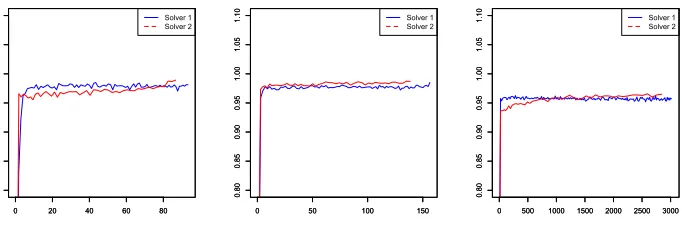
We also compute the statisticFn
def
= 2SennPrecn
Senn+Precn which measures the recovery of the
sparsity structure of θ∞along the iteration. In this definition Senn is the sensitivity,
and Precn is the precision defined as
Senn=
P
j<i1{|θn,ij|>0}1{|θ∞,ij|>0}
P
j<i1{|θ∞,ij|>0}
, and Precn =
P
j<i1{|θn,ij|>0}1{|θ∞,ij|>0}
P
j<i1{|θ∞,ij|>0}
.
2. this depends heavily onn,p, the actual true matrixθtrue, and depends also heavily the choice of
0 20 40 60 80 0.0 0.2 0.4 0.6 0.8 1.0
0 20 40 60 80
0.0 0.2 0.4 0.6 0.8 1.0 Solver 1 Solver 2
0 50 100 150
0.0 0.2 0.4 0.6 0.8 1.0
0 50 100 150
0.0 0.2 0.4 0.6 0.8 1.0 Solver 1 Solver 2
0 500 1000 1500 2000 2500 3000
0.0 0.2 0.4 0.6 0.8 1.0
0 500 1000 1500 2000 2500 3000
0.0 0.2 0.4 0.6 0.8 1.0 Solver 1 Solver 2
Figure 1: Relative errors plotted as function of computing time forSolver 1andSolver 2.
0 20 40 60 80
0.80 0.85 0.90 0.95 1.00 1.05 1.10
0 20 40 60 80
0.80 0.85 0.90 0.95 1.00 1.05
1.10 Solver 1
Solver 2
0 50 100 150
0.80 0.85 0.90 0.95 1.00 1.05 1.10
0 50 100 150
0.80 0.85 0.90 0.95 1.00 1.05
1.10 Solver 1
Solver 2
0 500 1000 1500 2000 2500 3000
0.80 0.85 0.90 0.95 1.00 1.05 1.10
0 500 1000 1500 2000 2500 3000
0.80 0.85 0.90 0.95 1.00 1.05
1.10 Solver 1
Solver 2
Figure 2: Statistic Fn plotted as function of computing time for Solver 1 and Solver
2.
The values of Fn are presented on Figure 2 as function of computing time. It shows
that for both solvers, the sparsity structure ofθn converges very quickly towards that
of θ∞. We note also that Figure 2 seems to suggest thatSolver 2 tends to produce solutions with slightly more stable sparsity structure than Solver 1 (less variance on the red curves). Whether such subtle differences exist between the two algorithms (a diminishing step-size and fixed Monte Carlo size versus a fixed step-size and increasing Monte Carlo size) is an interest question. Our analysis does not deal with the sparsity structure of the solutions, hence cannot offer any explanation.
5. A non convex example: High-dimensional logistic regression with random effects
sec-tion 2 and secsec-tion 3 provide useful informasec-tion to tune the design parameters of the algorithms.
5.1 The model
We model binary responses {Yi}Ni=1 ∈ {0,1} asN conditionally independent realiza-tions of a random effect logistic regression model,
Yi|U ind.
∼ Ber s(x0iβ+σzi0U)
, 1≤i≤N , (17)
wherexi∈Rp is the vector of covariates,zi ∈Rq are (known) loading vector, Ber(α)
denotes the Bernoulli distribution with parameterα∈[0,1],s(x) = ex/(1 + ex) is the
cumulative distribution function of the standard logistic distribution. The random effectU is assumed to be standard GaussianU∼Nq(0, I).
The log-likelihood of the observations at θ= (β, σ)∈Rp×(0,∞) is given by
`(θ) = log
Z N
Y
i=1
s(x0iβ+σzi0u)Yi 1−s(x0
iβ+σzi0u)
1−Yi
φ(u)du, (18)
whereφis the density of aRq-valued standard Gaussian random vector. The number
of covariates p is possibly larger than N, but only a very small number of these covariates are relevant which suggests to use the elastic-net penalty
λ
1−α 2 kβk
2
2+αkβk1
, (19)
where λ > 0 is the regularization parameter, kβkr = (Pp
i=1|βi|r)1/r and α ∈ [0,1]
controls the trade-off between the`1 and the`2 penalties. In this example, g(θ) =λ
1−α 2 kβk
2
2+αkβk1
+1(0,+∞)(σ), (20) where 1A(x) = +∞ is x /∈ A and 0 otherwise. Define the conditional log-likelihood
of Y= (Y1, . . . , YN) given U (the dependence uponY is omitted) by
`c(θ|u) = N
X
i=1
Yi x0iβ+σzi0u
−ln 1 + exp x0iβ+σz0iu ,
and the conditional distribution of the random effectUgiven the observationsYand the parameterθ
πθ(u) = exp (`c(θ|u)−`(θ))φ(u). (21)
The Fisher identity implies that the gradient of the log-likelihood (18) is given by
∇`(θ) =
Z
∇θ`c(θ|u) πθ(u) du=
Z ( N
X
i=1
(Yi−s(x0iβ+σz
0
iu))
xi zi0u
)
The Hessian of the log-likelihood ` is given by (see e.g.(McLachlan and Krishnan, 2008, Chapter 3))
∇2`(θ) =Eπθ
∇2θ`c(θ|U)
+ Covπθ(∇θ`c(θ|U))
whereEπθ and Covπθ denotes the expectation and the covariance with respect to the
distributionπθ, respectively. Since
∇2θ`c(θ|u) =− N
X
i=1
s(x0iβ+σz0iu) 1−s(x0iβ+σzi0u)
xi zi0u
xi zi0u
0
,
and supθ∈Θ
R
kuk2π
θ(u) du < ∞ (see section A), ∇2`(θ) is bounded on Θ. Hence,
∇`(θ) satisfies the Lipschitz condition showing that H1 is satisfied.
5.2 Numerical application
The assumption H3 is satisfied withπθ given by (21) and
Hθ(u) =− N
X
i=1
(Yi−F(x0iβ+σzi0u))
xi zi0u
. (22)
The distribution πθ is sampled using the MCMC sampler proposed in Polson et al.
(2013) based on data-augmentation. We write−∇`(θ) =R
Rq×RNHθ(u)˜πθ(u,w) dudw where ˜πθ(u,w) is defined foru∈Rq and w= (w1,· · ·, wN)∈RN by
˜
πθ(u,w) = N
Y
i=1 ¯
πPG wi;x0iβ+σz
0
iu
!
πθ(u) ;
in this expression, ¯πPG(·;c) is the density of the Polya-Gamma distribution on the
positive real line with parameter cgiven by
¯
πPG(w;c) = cosh(c/2) exp −wc2/2
ρ(w)1R+(w),
whereρ(w)∝P
k≥0(−1)k(2k+ 1) exp(−(2k+ 1)2/(8w))w
−3/2 (see (Biane et al., 2001, Section 3.1)). Thus, we have
˜
πθ(u,w) =Cθφ(u) N
Y
i=1
exp σ(Yi−1/2)zi0u−wi(x0iβ+σz0iu)2/2
ρ(wi)1R+(wi),
where lnCθ =−Nln 2−`(θ) +PiN=1(Yi−1/2)x0iβ. This target distribution can be
sampled using a Gibbs algorithm: given the current value (ut,wt) of the chain, the next point is obtained by samplingut+1under the conditional distribution ofu given wt, andwt+1 under the conditional distribution ofwgivenut+1. In the present case, these conditional distributions are given respectively by
˜
πθ(u|w)≡Nq(µθ(w); Γθ(w)) π˜θ(w|u) = N
Y
i=1 ¯
with
Γθ(w) = I+σ2 N
X
i=1 wizizi0
!−1
, µθ(w) =σΓθ(w) N
X
i=1
(Yi−1/2)−wix0iβ
zi .
(23) Exact samples of these conditional distributions can be obtained (see (Polson et al., 2013, Algorithm 1) for sampling under a Polya-Gamma distribution). It has been shown by Choi and Hobert (2013) that the Polya-Gamma Gibbs sampler is uniformly ergodic. Hence H5 is satisfied withW ≡1. Checking H6 is also straightforward.
We test the algorithms withN = 500,p= 1,000 andq= 5. We generate theN×p covariates matrix X columnwise, by sampling a stationary RN-valued autoregressive
model with parameter ρ = 0.8 and Gaussian noise p1−ρ2N
N(0, I). We generate
the vector of regressorsβtrue from the uniform distribution on [1,5] and randomly set
98% of the coefficients to zero. The variance of the random effect is set to σ2 = 0.1. We consider a repeated measurement setting so thatzi =ediq/Newhere{ej, j≤q} is
the canonical basis ofRq andd·e denotes the upper integer part. With such a simple
expression for the random effect, we will be able to approximate the value F(θ) in order to illustrate the theoretical results obtained in this paper. We use the Lasso penalty (α= 1 in (19)) withλ= 30.
We first illustrate the ability of Monte Carlo Proximal Gradient algorithms to find a minimizer of F. We compare the Monte Carlo proximal gradient algorithm
(i) with fixed batch size: γn = 0.01/
√
n and mn = 275 (Algo 1); γn = 0.5/n and mn= 275 (Algo 2).
(ii) with increasing batch size: γn = γ = 0.005, mn = 200 +n (Algo 3); γn = γ = 0.001, mn = 200 +n (Algo 4); andγn = 0.05/
√
n and mn = 270 +d
√
ne
(Algo 5).
Each algorithm is run for 150 iterations. The batch sizes {mn, n ≥ 0} are chosen
so that after 150 iterations, each algorithm used approximately the same number of Monte Carlo samples. We denote by β∞ the value obtained at iteration 150. A path of the relative error kβn−β∞k/kβ∞k is displayed on Figure 3[right] for each algorithm; a path of the sensitivitySenn and of the precisionPrecn(see section 4 for
the definition) are displayed on Figure 4. All these sequences are plotted versus the total number of Monte Carlo samples up to iteration n. These plots show that with a fixed batch-size (Algo 1 or Algo 2), the best convergence is obtained with a step size decreasing as O(1/√n); and for an increasing batch size (Algo 3 to Algo 5), it is better to choose a fixed step size. These findings are consistent with the results in section 3. On Figure 3[left], we report on the bottom row the indices j such that βtrue,j is non null and on the rows above, the indices jsuch thatβ∞,j given by Algo 1
to Algo 5 is non null.
We now study the convergence of {F(θn), n∈N} whereθn is obtained by one of
0 100 200 300 400 500 600 700 800 900 1000 Beta True
Algo 5 Algo 4 Algo 3 Algo 2 Algo 1
0 0.5 1 1.5 2 2.5 3 3.5 4
x 104 10−4
10−2 100 102 104
0 0.5 1 1.5 2 2.5 3 3.5 4
x 104 10−4
10−2 100 102 104
Algo 1 Algo 2
Algo 3 Algo 4 Algo5
Figure 3: [left] The support of the sparse vector β∞ obtained by Algo 1 to Algo 5; for comparison, the support ofβtrue is on the bottom row. [right] Relative
error along one path of each algorithm as a function of the total number of Monte Carlo samples.
0 0.5 1 1.5 2 2.5 3 3.5 4
x 104 0
0.2 0.4 0.6 0.8 1
Algo 1 Algo 2
0 0.5 1 1.5 2 2.5 3 3.5 4
x 104 0
0.2 0.4 0.6 0.8 1
Algo 3 Algo 4 Algo5
0 0.5 1 1.5 2 2.5 3 3.5 4
x 104 0
0.2 0.4 0.6 0.8 1
Algo 1 Algo 2
0 0.5 1 1.5 2 2.5 3 3.5 4
x 104 0
0.2 0.4 0.6 0.8 1
Algo 3 Algo 4 Algo5
Figure 4: The sensitivity Senn [left] and the precision Precn [right] along a path,
0 50 100 150 102
103 104 105
0 0.5 1 1.5 2 2.5 3 3.5 4
x 104 102
103 104 105
Algo 1 Algo 3
Algo 1 Algo 3
0 0.5 1 1.5 2 2.5 3 3.5 4
x 104 103
104
Algo 1 Algo 3 Algo 4
Figure 5: [left] n7→ F(θn) for several independent runs. [right] E[F(θn)] versus the
total number of Monte Carlo samples up to iterationn
that all the paths have the same limiting value, which is approximately F? = 311;
we observed the same behavior on the 50 runs of each algorithm. On Figure 5[right], we report the Monte Carlo estimation of E[F(θn)] versus the total number of Monte
Carlo samples used up to iteration n for the best strategies in the fixed batch size case (Algo 1) and in the increasing batch size case (Algo 3 and Algo 4).
6. Proofs
6.1 Preliminary lemmas
Lemma 7 Assume that g is lower semi-continuous and convex. For θ, θ0 ∈ Θ and γ >0
gProxγ,g(θ)
−g(θ0)≤ −1
γ
Proxγ,g(θ)−θ0,Proxγ,g(θ)−θ
. (24)
For any γ >0 and for any θ, θ0 ∈Θ,
kProxγ,g(θ)−Proxγ,g(θ0)k2+k Proxγ,g(θ)−θ
− Proxγ,g(θ0)−θ0
k2 ≤ kθ−θ0k2 . (25) Proof See (Bauschke and Combettes, 2011, Propositions 4.2., 12.26 and 12.27).
Lemma 8 Assume H1 and let γ ∈(0,1/L]. Then for all θ, θ0 ∈Θ,
−2γ
F(Proxγ,g(θ))−F(θ0)
≥ kProxγ,g(θ)−θ0k2+ 2
Proxγ,g(θ)−θ0, θ0−γ∇f(θ0)−θ
. (26)
If in addition f is convex, then for all θ, θ0, ξ ∈Θ,
−2γ
F Proxγ,g(θ)
−F(θ0)
≥ kProxγ,g(θ)−θ0k2
+ 2Proxγ,g(θ)−θ0, ξ−γ∇f(ξ)−θ
Proof Since ∇f is Lipschitz, the descent lemma implies that for any γ−1≥L f(p)−f(θ0)≤
∇f(θ0), p−θ0
+ 1
2γkp−θ
0k2 . (28)
This inequality applied with p = Proxγ,g(θ) combined with (24) yields (26). When f is convex, f(ξ) +h∇f(ξ), θ0−ξi −f(θ0) ≤0 which, combined again with (24) and (28) applied with (p, θ0)←(Proxγ,g(θ), ξ) yields the result.
Lemma 9 Assume H1. Then for any γ >0, θ, θ0∈Θ,
kθ−γ∇f(θ)−θ0+γ∇f(θ0)k ≤(1 +γL)kθ−θ0k, (29)
kTγ(θ)−Tγ(θ0)k ≤(1 +γL)kθ−θ0k. (30)
If in addition f is convex then for any γ ∈(0,2/L],
kθ−γ∇f(θ)−θ0+γ∇f(θ0)k ≤ kθ−θ0k, (31)
kTγ(θ)−Tγ(θ0)k ≤ kθ−θ0k. (32)
Proof (30) and (32) follows from (29) and (31) respectively by the Lipschitz property of the proximal map Proxγ,g (see Lemma 7). (29) follows directly from the Lipschitz
property of f. It remains to prove (31). Since f is a convex function with Lipschitz-continuous gradients, (Nesterov, 2004, Theorem 2.1.5) shows that, for all θ, θ0 ∈ Θ, L h∇f(θ)− ∇f(θ0), θ−θ0i ≥ k∇f(θ)− ∇f(θ0)k2. The result follows.
Lemma 10 Assume H1. Set Sγ(θ) def= Proxγ,g(θ−γH) and η def= H− ∇f(θ). For
anyθ∈Θ and γ >0,
kTγ(θ)−Sγ(θ)k ≤γkηk. (33)
Proof We have kTγ(θ)−Sγ(θ)k =kProxγ,g(θ−γ∇f(θ))−Proxγ,g(θ−γH)k and
(33) follows from Lemma 7.
6.2 Proof of section 2
6.2.1 Proof of Lemma 1
Setwn=vn+Pk≥n+1ξk+M with M
def
= −infnPk≥nξk so that infnwn≥0. Then
0≤wn+1 ≤vn−χn+1+ξn+1+
X
k≥n+2
ξk+M ≤wn−χn+1 .
{wn, n∈N}is non-negative and non increasing; therefore it converges. Furthermore,
0≤Pn
k=0χk≤w0 so that
P
nχn<∞. The convergence of{wn, n∈N}also implies
6.2.2 Proof of Theorem 2
Let θ? ∈ L, which is not empty by H2; note that F(θ?) = minF. We have by (27)
applied with θ←θn−γn+1Hn+1,ξ←θn,θ0 ←θ?,γ ←γn+1
kθn+1−θ?k2≤ kθn−θ?k2−2γn+1(F(θn+1)−minF)−2γn+1hθn+1−θ?, ηn+1i . We write θn+1 −θ? = θn+1 −Tγn+1(θn) +Tγn+1(θn)−θ?. By Lemma 10, kθn+1 − Tγn+1(θn)k ≤γn+1kηn+1k so that,
− hθn+1−θ?, ηn+1i ≤γn+1kηn+1k2−
Tγn+1(θn)−θ?, ηn+1
.
Hence,
kθn+1−θ?k2 ≤ kθn−θ?k2−2γn+1(F(θn+1)−minF)
+ 2γn2+1kηn+1k2−2γn+1
Tγn+1(θn)−θ?, ηn+1
. (34)
Under (7) and (34), Lemma 1 shows thatP
nγn(F(θn)−minF)<∞and limnkθn− θ?k exists. This implies that supnkθnk < ∞. Since Pnγn = +∞, there exists a
subsequence{θφn, n∈N}such that limnF(θφn) = minF. The sequence {θφn, n≥0}
being bounded, we can assume without loss of generality that there exists θ∞ ∈ Rd
such that limnθφn=θ∞.
Let us prove thatθ∞∈ L. Sincegis lower semi-continuous on Θ, lim infng(θφn)≥
g(θ∞) so thatθ∞∈Θ. Since F is lower semi-continuous on Θ, we have
minF = lim inf
n→∞ F(θφn)≥F(θ∞)≥minF , showing that F(θ∞) = minF.
By (34), for any m and n≥φm
kθn+1−θ∞k2≤ kθφm−θ∞k
2−2
n
X
k=φm
γk+1{
Tγk+1(θk)−θ∞, ηk+1
+γk+1kηk+1k2}.
For any > 0, there existsm such that the RHS is upper bounded by . Hence, for any n≥φm,kθn+1−θ∞k2 ≤, which proves the convergence of{θn, n∈N} toθ∞.
6.2.3 Proof of Theorem 3
Let θ? ∈ L; note thatF(θ?) = minF. We first apply (27) withθ ← θj −γj+1Hj+1, ξ←θj,θ0←θ?,γ ←γj+1:
F(θj+1)−minF ≤(2γj+1)−1 kθj−θ?k2− kθj+1−θ?k2
− hθj+1−θ?, ηj+1i . Multiplying both sides by aj+1 gives:
aj+1
F(θj+1)−minF
≤ 1
2
aj+1 γj+1
−aj
γj
kθj−θ?k2+ aj
2γj
kθj−θ?k2
− aj+1
2γj+1
Summing fromj = 0 to n−1 gives
an
2γn
kθn−θ?k2+ n
X
j=1
aj{F(θj)−minF} ≤
1 2
n
X
j=1
aj γj
−aj−1
γj−1
kθj−1−θ?k2
−
n
X
j=1
ajhθj−θ?, ηji+ a0 2γ0
kθ0−θ?k2. (35)
We decompose hθj−θ?, ηji as follows:
hθj−θ?, ηji=
θj−Tγj(θj−1), ηj
+Tγj(θj−1)−θ?, ηj
.
By Lemma 10, we get
θj−Tγj(θj−1), ηj
≤γjkηjk2 which concludes the proof.
6.3 Proof of Section 3.1
The proof of Theorem 4 is given in the case m = 1; we simply denote by Xn the
sample Xn(1). The proof for the casem >1 can be adapted from the proof below, by
substituting the functions Hθ(x) and W(x) by
Hθ(x1,· · · , xm) =
1 m
m
X
k=1
Hθ(xk) W(x1,· · ·, xm) =
1 m
m
X
k=1
W(xk) ;
the kernelPθ and its invariant measureπθ by
Pθ(x1,· · · , xm;B) =
Z
· · ·
Z
Pθ(xm,dy1)
m
Y
k=2
Pθ(yk−1,dyk)1B(y1, . . . , ym),
πθ(B) =
Z
· · ·
Z
πθ(dy1) m
Y
k=2
Pθ(yk−1,dyk)1B(y1, . . . , ym),
for any (x1, . . . , xm)∈Xn andB ∈ X×n.
6.3.1 Preliminary results
Proposition 11 Assume that g is proper convex and Lipschitz on Θ with Lipschitz constant K. Then, for all θ∈Θ,
kProxγ,g(θ)−θk ≤Kγ . (36)
Proof For all θ∈Θ, we get by Lemma 7
Proposition 12 Assume H1, H2 and Θis bounded. Then sup
γ∈(0,1/L] sup
θ∈Θ
kTγ(θ)k<∞.
If in addition H6-(ii) holds, then there exists a constantC such that for any θ,θ¯∈Θ, γ,¯γ ∈(0,1/L]
Tγ(θ)−Tγ¯(¯θ)
≤C γ+ ¯γ+kθ−θ¯k
.
Proof Let θ? such that for any γ >0, θ? =Tγ(θ?) (such a point exists by H2 and
(4)). We writeTγ(θ) = (Tγ(θ)−θ?)+θ?. By Lemma 9, there exists a constantCsuch
that for any θ∈Θ and any γ ∈(0,1/L], kTγ(θ)−θ?k ≤2 kθ−θ?k ≤2kθk+ 2kθ?k.
This concludes the proof of the first statement. We write Tγ(θ)−Tγ¯(¯θ) = Tγ(θ)− T¯γ(θ) +T¯γ(θ)−Tγ¯(¯θ). By Lemma 7
T¯γ(θ)−Tγ¯(¯θ)
≤
θ−θ¯−γ¯∇f(θ) + ¯γ∇f(¯θ)
≤ kθ−θ¯k+ ¯γsup
θ∈Θ
k∇f(θ)k.
By H1 and since Θ is bounded, supθ∈Θk∇f(θ)k < ∞. In addition, using again Lemma 7,
kTγ(θ)−Tγ¯(θ)k ≤(γ+ ¯γ) sup
θ∈Θ
k∇f(θ)k+kProxγ,g(θ)−Prox¯γ,g(θ)k .
We conclude by using
kProx¯γ,g(θ)−Proxγ,g(θ)k ≤ kProxγ,g¯ (θ)−θk+kθ−Proxγ,g(θ)k
≤(γ+ ¯γ) sup
γ∈(0,1/L] sup
θ∈Θ
γ−1 kProxγ,g(θ)−θk .
Lemma 13 Assume H5 and H6-(i).
(i) There exists a measurable function(θ, x)7→Hbθ(x)such thatsupθ∈Θ
Hbθ
W <
∞
and for any (θ, x)∈Θ×X,
b
Hθ(x)−PθHbθ(x) =Hθ(x)− Z
Hθ(y)πθ(dy). (37)
(ii) There exists a constant C such that for any θ, θ0∈Θ,
PθHbθ−Pθ0Hbθ0
W ≤C
θ−θ0
.
Lemma 14 Assume H4 and H5. Then, supnE[Wp(Xn)]<∞.
Proof The conditional distribution of Xj given the past Fj−1 is Pθj−1(Xj−1,·). Therefore, we write
E[Wp(Xn)] =E[E[Wp(Xn)| Fn−1]] =EPθn−1W
p(X n−1)
.
We then use the drift inequality to obtain E[Wp(Xn)] ≤ λE[Wp(Xn−1)] +b. The proof then follows from a trivial induction.
Lemma 15 Assume H1, H6-(ii) and Θ is bounded. There exists a constant C such that w.p.1, for all n≥0,
kθn+1−θnk ≤Cγn+1(1 +kηn+1k) .
Proof We write
θn+1−θn=θn+1−Proxγn+1,g(θn) + Proxγn+1,g(θn)−θn. Since by Lemma 7,θ7→Proxγ,g(θ) is Lipschitz for anyγ >0, we get
θn+1−Proxγn+1,g(θn)
=Proxγn+1,g(θn−γn+1ηn+1−γn+1∇f(θn))−Proxγn+1,g(θn)
≤γn+1kηn+1+∇f(θn)k ≤γn+1
kηn+1k+ sup
θ∈Θ
k∇f(θ)k
.
By H1, w.p.1. supθ∈Θk∇f(θ)k< ∞; hence, there exists C1 such that w.p.1. for all n≥0, θn+1−Proxγn+1,g(θn)
≤C1γn+1(1 +kηn+1k). Finally, under H6-(ii), there
exists a constant C2 such that, w.p.1., sup
n
γn−+11 Proxγn+1,g(θn)−θn
≤ sup
γ∈(0,1/L] sup
θ∈Θ
γ−1kProxγ,g(θ)−θk ≤C2 .
This concludes the proof.
Lemma 16 Assume H1, H4, H5 and Θis bounded. There exists a constant C such that w.p.1, for all n≥0, kηn+1k ≤CW(Xn+1).
6.3.2 Proof of Theorem 4
The proof of the almost-sure convergence consists in verifying the assumptions of Theorem 2. Let us start with the proof that almost-surely, P
nγn2+1kηn+1k2 < ∞. This property is a consequence of Lemma 17 applied with an ← γn2. It remains to
prove that almost-surely
X
n
γnηn<∞,
X
n γn+1
Tγn+1(θn), ηn+1
<∞;
note that they are both of the form P
nγn+1Aγn+1(θn)ηn+1 with, respectively, Aγ(θ) equal to the identity matrix, andAγ(θ) =Tγ(θ). In the case the Monte Carlo is
unbi-ased, we apply Proposition 18 with an←γn and Aγ(θ) equal to the identity matrix
and we obtain the almost-sure convergence ofP
nγnηn; we then apply Proposition 18
with an ← γn and Aγ(θ) = Tγ(θ), and we obtain the almost-sure convergence of
P
nγn+1
Tγn+1(θn), ηn+1
- note that by Proposition 12, Tγ(θ) satisfies the
assump-tions on Aγ(θ). In the case the Monte Carlo is biased, the steps are the same except
we use Proposition 19 instead of Proposition 18.
For the control of the moments, we use Theorem 3 and again Lemma 17 and Proposition 18 for the unbiased case (or Proposition 19 for the biased case).
Lemma 17 Assume H1, H4, H5 andΘ is bounded.
(i) If ak≥0 and P∞k=1ak<∞ then with probability one, Pn≥1ankηnk2<∞. (ii) for any q ∈ [1, p/2], there exists a constant C such that for any non-negative
numbers {a1,· · · , an},
n
X
k=1
akkηkk2
Lq
≤C n
X
k=1 ak.
Proof We write
E
X
n≥0
an+1kηn+1k2
≤sup
n E
kηn+1k2
X
n≥0 an+1 .
By Lemma 14 and Lemma 16, supnkηn+1kL2 < ∞ so the RHS is finite. By the Minkovski inequality, we write sinceak>0,
n
X
k=0
ak+1kηk+1k2
Lq
≤sup
n
kηnk2L2q n+1
X
k=1 ak.
The supremum is finite by Lemma 14 and Lemma 16.
Proposition 18 Assume H1, H3, H4, H5, Θ is bounded and the Monte Carlo ap-proximation is unbiased. Let {an, n ∈ N} be a deterministic positive sequence and
{Aγ(θ), γ∈(0,1/L], θ∈Θ} be deterministic matrices such that
sup
γ∈(0,1/L] sup
θ∈Θ
(i) If P
n≥0a2n<∞, then the series
P
n≥0an+1Aγn+1(θn)ηn+1 converges P-a.s. (ii) For any q∈(1, p/2], there exists a constant C such that
n X k=0
ak+1Aγk+1(θk)ηk+1
Lq ≤C n X k=0 a2k+1
!1/2
.
Proof Since θn ∈ Fn, we have Ean+1Aγn+1(θn) ηn+1|Fn
= 0, thus showing that
{Mn =Pnk=0ak+1Aγk+1(θk)ηk+1, n ∈N} is a martingale. This martingale converges almost-surely if S = P
n≥0a2n+1kAγn+1(θn)k 2kη
n+1k2 < ∞ P-a.s. (see e.g. (Hall and
Heyde, 1980, Theorem 2.17)). Using (38) and Lemma 17,S <∞ P-a.s.
Consider now the Lq-moment ofMn. We apply (Hall and Heyde, 1980, Theorem
2.10): for anyq ∈(1, p/2], there exists a constant C such that for anyn≥0,
n X k=0
ak+1Aγk+1(θk)ηk+1
Lq ≤C n X k=0
ak+1Aγk+1(θk)ηk+1
2
Lq
!1/2
.
Lemma 14 and Lemma 16 imply that supnkηn+1kLq < ∞; we then conclude with
(38).
Proposition 19 Assume H1, H3–H6 andΘis bounded. Let {an, n≥0} be a positive
sequence and{Aγ(θ), γ∈(0,1/L], θ∈Θ} be (deterministic) function-valued matrices
such that there exists CA and for any γ,γ¯∈(0,1/L]and θ,θ¯∈Θ
sup
γ∈(0,1/L] sup
θ∈Θ
kAγ(θ)k<∞,
Aγ(θ)−A¯γ(¯θ)
≤CA γ+ ¯γ+
θ−θ¯
. (39)
(i) If P
nanγn < ∞,
P
na2n < ∞ and
P
n|an+1 − an| < ∞ then the series
P
n≥0an+1Aγn+1(θn)ηn+1 converges P-a.s.
(ii) For any q∈(1, p/2], there exists a constant C such that
n X k=0
ak+1Aγk+1(θk)ηk+1
Lq ≤C 1 + n X k=0 a2k+1
!1/2
+
n
X
k=1
|ak+1−ak|+ n
X
k=1 akγk
.
Proof
(i) By H4 and Lemma 13-(i), we write
ηn+1=Hbθn(Xn+1)−PθnHbθn(Xn+1)
=
b
Hθn(Xn+1)−PθnHbθn(Xn)
+
PθnHbθn(Xn)−Pθn+1Hbθn+1(Xn+1)
+Pθn+1Hbθn+1(Xn+1)−PθnHbθn(Xn+1)
We prove successively that w.p.1,
X
n
an+1Aγn+1(θn)
b
Hθn(Xn+1)−PθnHbθn(Xn)
<∞, (40)
X
n≥0
an+1Aγn+1(θn)
PθnHbθn(Xn)−Pθn+1Hbθn+1(Xn+1)
<∞, (41)
X
n≥0
an+1Aγn+1(θn)
Pθn+1Hbθn+1(Xn+1)−PθnHbθn(Xn+1)
<∞. (42)
Proof [Proof of (40)] By H4, {Hbθn(Xn+1)−PθnHbθn(Xn), n ∈ N} is a martingale
increment w.r.t. the filtration {Fn, n≥0}. The proof is along the same lines as the
proof of Proposition 18 upon noting that by Lemma 13 and H5, there exists C such that w.p.1 for all n≥0,
kHbθn(Xn+1)−PθnHbθn(Xn)k ≤C {W(Xn+1) +W(Xn)} .
Proof [Proof of (41)] The sum is equal to P
n≥0∆n+1PθnHbθn(Xn) with ∆n+1 =
an+1Aγn+1(θn)−anAγn(θn−1). On one hand, by Lemma 13 and H5, there exists C
such that w.p.1 for all n≥0,
PθnHbθn(Xn)
≤C W(Xn).
On the other hand, by (39), Lemma 15 and Lemma 16, there exists C such that a.s.
for alln≥0, k∆n+1k ≤C
|an+1−an|+an(γn+γn+1)
W(Xn).
By Lemma 14, supnEW2(Xn)
< ∞. Therefore, by (39) and the assumptions on
{an, n≥0}, we havePnE h
∆n+1 PθnHbθn(Xn)
i
<∞; which concludes the proof.
Proof [Proof of (42)] By (39) and Lemma 13, there exists a constant C such that w.p.1 for any n
Aγn+1(θn)
Pθn+1Hbθn+1(Xn+1)−PθnHbθn(Xn+1)
≤C kθn+1−θnk W(Xn+1).
By Lemma 15 and Lemma 16, there exists a constantC such that w.p.1,
for all n≥0, kθn+1−θnkW(Xn+1)≤Cγn+1W2(Xn+1).
From Lemma 14 and the assumptions on {an, n≥0},Pnan+1γn+1EW2(Xn+1)
<
(ii) We start from the same decomposition of ηn+1 in three terms. The first one is a martingale, and following the same lines as in the proof of Proposition 18, we obtain n X k=0
ak+1Aγn+1(θn)
b
Hθn(Xn+1)−PθnHbθn(Xn)
Lq ≤C n X k=0 a2k+1
!1/2
.
For the second term, we write
n
X
k=0
ak+1Aγk+1(θk)
PθkHbθk(Xk)−Pθk+1Hbθk+1(Xk+1)
≤a1Aγ1(θ0)Pθ0Hbθ0(X0)−an+1Aγn+1(θn)Pθn+1Hbθn+1(Xn+1)
+
n
X
k=1
∆k+1 PθkHbθk(Xk).
By the Minkovski inequality, it is easily seen that there exists a constantCsuch that
n X k=0
ak+1Aγk+1(θk)
PθkHbθk(Xk)−Pθk+1Hbθk+1(Xk+1)
Lq
≤ 1 +an+1+
n
X
k=1
|ak+1−ak|+ak(γk+γk+1)
!
.
Finally, for the last term, following the same computations as above, we have by the Minkovski inequality n X k=0
ak+1Aγk+1(θk)
Pθk+1Hbθk+1(Xk+1)−PθkHbθk(Xk+1)
Lq ≤C n X k=0
ak+1γk+1 .
6.4 Proof of Theorem 6
We writeηn+1 =Bn+ (ηn+1−Bn) whereBnis given by (12). Observe that{ηn+1− Bn, n∈N} is a martingale-increment sequence. Sufficient conditions for the
almost-sure convergence of a martingale and the control ofLq-moments can be found in (Hall and Heyde, 1980, Theorems 2.10 and 2.17). Then the proof follows from Proposition 5 and Lemma 14.
Appendix A. Proofs of section 4
By using the Cauchy-Schwartz inequality, it holds
Z
exp(`c(θ|u))φ(u)du≥
Z
exp(0.5`c(θ|u))φ(u)du
Z
exp(`c(θ|u))kuk2φ(u) du
2
≤
Z
exp(0.5`c(θ|u))φ(u) du
Z
exp(3`c(θ|u)/2)kuk4φ(u)du
which implies that
Z
kuk2πθ(u)du=
R
exp(`c(θ|u))kuk2φ(u)du
R
exp(`c(θ|v))φ(v)dv
≤
Z
exp (3`c(θ|u)/2)kuk4φ(u) du
1/2
Since exp(`c(θ|u))≤1 and
R
kuk4φ(u)du=q(2 +q), we have sup
θ∈Θ
Z
kuk2π
θ(u)du≤
p
q(2 +q).
Appendix B. Proof of section 5
Forθ, ϑ∈Θ, the (i, j)-th entry of the matrix ∇`(θ)− ∇`(ϑ) is given by
(∇`(θ)− ∇`(ϑ))ij =
Z
Xp
¯
Bij(x)πϑ(dx)−
Z
Xp
¯
Bij(x)πθ(dx).
Fort∈[0,1] let
πt(dz)
def
= exp
¯
B(z), tϑ+ (1−t)θ
R
exp ¯
B(x), tϑ+ (1−t)θ
µ(dx), defines a probability measure on Xp. It is straightforward to check that
(∇`(θ)− ∇`(ϑ))ij =
Z
¯
Bij(x)π1(dx)−
Z
¯
Bij(x)π0(dx),
and thatt7→R ¯
Bij(x)πt(dx) is differentiable with derivative
d dt
Z
¯
Bij(x)πt(dx)
=
Z
¯ Bij(x)
¯ B(x)−
Z
¯
B(z)πt(dz), ϑ−θ
πt(dx),
=Covπt B¯ij(X),
¯
B(X), ϑ−θ,
where the covariance is taken assuming thatX ∼πt. Hence
(∇`(θ)− ∇`(ϑ))ij
= Z 1 0
dt Covt B¯ij(X),
¯
B(X), ϑ−θ
≤osc( ¯Bij)
s X
k≤l
osc2( ¯B
kl)kθ−ϑk2. This implies the inequality (16).
References
S. Allassonni`ere and E. Kuhn. Convergent Stochastic Expectation Maximization algorithm with efficient sampling in high dimension. Application to deformable template model estimation. Comput. Stat. Data An., 91:4–19, 2015.
C. Andrieu and E. Moulines. On the ergodicity properties of some adaptive MCMC algorithms. Ann. Appl. Probab., 16(3):1462–1505, 2006.
C. Andrieu, E. Moulines, and P. Priouret. Stability of stochastic approximation under verifiable conditions. SIAM J. Control Optim., 44(1):283–312, 2005.
O. Banerjee, L. El Ghaoui, and A. d’Aspremont. Model selection through sparse maximum likelihood estimation for multivariate Gaussian or binary data. J. Mach. Learn. Res., 9:485–516, 2008.
H. Bauschke and P.L. Combettes. Convex analysis and monotone operator theory in Hilbert spaces. CMS Books in Mathematics/Ouvrages de Math´ematiques de la SMC. Springer, New York, 2011. ISBN 978-1-4419-9466-0. With a foreword by H´edy Attouch.
A. Beck and M. Teboulle. Gradient-based algorithms with applications to signal-recovery problems. In Convex optimization in signal processing and communica-tions, pages 42–88. Cambridge Univ. Press, Cambridge, 2010.
A. Benveniste, M. M´etivier, and P. Priouret. Adaptive algorithms and stochastic approximations, volume 22 of Applications of Mathematics (New York). Springer-Verlag, Berlin, 1990.
P. Biane, J. Pitman, and M. Yor. Probability laws related to the Jacobi theta and Riemann zeta functions, and Brownian excursions. Bull. Amer. Math. Soc. (N.S.), 38(4):435–465 (electronic), 2001. ISSN 0273-0979.
H.M. Choi and J. P. Hobert. The polya-gamma gibbs sampler for bayesian logistic regression is uniformly ergodic. Electronic Journal of Statistics, 7:2054–2064, 2013.
P.L. Combettes. Inherently parallel Algorithms in Feasibility and Optimization and their Applications, chapter Quasi-Fejerian analysis of some optimization algorithms, pages 115–152. Elsevier Science, 2001.
P.L. Combettes and J.C. Pesquet. Proximal splitting methods in signal processing. In Fixed-point algorithms for inverse problems in science and engineering, volume 49 of Springer Optim. Appl., pages 185–212. Springer, New York, 2011.
P.L. Combettes and J.C. Pesquet. Stochastic Quasi-Fejer block-coordinate fixed point iterations with random sweeping. SIAM J. Optim., 25(2):1221–1248, 2015a.
P.L. Combettes and V. Wajs. Signal recovery by proximal forward-backward splitting. Multiscale Modeling and Simulation, 4(4):1168–1200, 2005.
A. Cotter, O. Shamir, N. Srebro, and K. Sridharan. Better mini-batch algorithms via accelerated gradient methods. In J. Shawe-Taylor, R. S. Zemel, P. L. Bartlett, F. Pereira, and K. Q. Weinberger, editors, Advances in Neural Information Pro-cessing Systems 24, pages 1647–1655. Curran Associates, Inc., 2011.
J. Duchi, E. Hazan, and Y. Singer. Adaptive subgradient methods for online learning and stochastic optimization. J. Mach. Learn. Res., 12:2121–2159, 2011. ISSN 1532-4435.
M. Ekeberg, C. L¨ovkvist, Y. Lan, M. Weigt, and E. Aurell. Improved contact predic-tion in proteins: Using pseudolikelihoods to infer potts models. Phys. Rev. E, 87: 012707, 2013.
G. Fort and E. Moulines. Convergence of the Monte Carlo expectation maximization for curved exponential families. Ann. Statist., 31(4):1220–1259, 2003. ISSN 0090-5364.
G. Fort, E. Moulines, and P. Priouret. Convergence of adaptive and interacting Markov chain Monte Carlo algorithms. Ann. Statist., 39(6):3262–3289, 2011. ISSN 0090-5364.
G. Fort, E. Moulines, M. Vihola, and A. Schreck. Convergence of Markovian Stochas-tic Approximation with discontinuous dynamics. Technical report, arXiv math.ST 1403.6803, 2014.
G. Fort, B. Jourdain, E. Kuhn, T. Leli`evre, and G. Stoltz. Convergence of the Wang-Landau algorithm. Mathematics of Computation, 84:2297–2327, 2015.
C.J. Geyer. On the convergence of Monte Carlo maximum likelihood calculations. J. Roy. Statist. Soc. Ser. B, 56(1):261–274, 1994.
J. Guo, E. Levina, G. Michailidis, and J. Zhu. Joint structure estimation for categor-ical Markov networks. Techncategor-ical report, Univ. of Michigan, 2010.
P. Hall and C.C. Heyde. Martingale Limit Theory and its Application. Academic Press, 1980.
H. H¨ofling and R. Tibshirani. Estimation of sparse binary pairwise Markov networks using pseudo-likelihoods. J. Mach. Learn. Res., 10:883–906, 2009.
C. Hu, W. Pan, and J.T. Kwok. Accelerated gradient methods for stochastic opti-mization and online learning. In Y. Bengio, D. Schuurmans, J. Lafferty, C. K. I Williams, and A. Culotta, editors,Advances in Neural Information Processing Sys-tems, pages 781–789, 2009.
![Figure 4: The sensitivity Senn [left] and the precision Precn [right] along a path,versus the total number of Monte Carlo samples up to time n](https://thumb-us.123doks.com/thumbv2/123dok_us/9783054.1963711/18.612.103.419.146.273/figure-sensitivity-precision-precn-versus-number-monte-samples.webp)
![Figure 5: [left] n �→ F(θn) for several independent runs. [right] E [F(θn)] versus thetotal number of Monte Carlo samples up to iteration n](https://thumb-us.123doks.com/thumbv2/123dok_us/9783054.1963711/19.612.124.418.99.228/figure-independent-versus-thetotal-monte-carlo-samples-iteration.webp)
