RecurJac: An Efficient Recursive Algorithm for Bounding Jacobian Matrix of Neural Networks and Its Applications

The Thirty-Third AAAI Conference on Artificial Intelligence (AAAI-19)

RecurJac: An Efficient Recursive Algorithm for

Bounding Jacobian Matrix of Neural Networks and Its Applications

Huan Zhang

UCLA [email protected]

Pengchuan Zhang

Microsoft Research AI [email protected]

Cho-Jui Hsieh

UCLA [email protected]

Abstract

The Jacobian matrix (or the gradient for single-output net-works) is directly related to many important properties of neural networks, such as the function landscape, stationary points, (local) Lipschitz constants and robustness to adver-sarial attacks. In this paper, we propose arecursivealgorithm, RecurJac, to compute both upper and lower bounds for each element in the Jacobian matrix of a neural network with re-spect to network’s input, and the network can contain a wide range of activation functions. As a byproduct, we can effi-ciently obtain a (local) Lipschitz constant, which plays a cru-cial role in neural network robustness verification, as well as the training stability of GANs. Experiments show that (lo-cal) Lipschitz constants produced by our method is of better quality than previous approaches, thus providing better ro-bustness verification results. Our algorithm has polynomial time complexity, and its computation time is reasonable even for relatively large networks. Additionally, we use our bounds of Jacobian matrix to characterize the landscape of the neural network, for example, to determine whether there exist sta-tionary points in a local neighborhood.

Introduction

Deep neural networks have been successfully applied to many applications, but one of the major criticisms is their being black boxes—no satisfactory explanation of their be-havior can be easily offered. Given a neural network fp¨q with inputx, one fundamental question to ask is: how does a perturbation in the input space affect the output predic-tion? To formally answer this question and bound the be-havior of neural networks, a critical step to answer this question is to compute the uniform bounds of the Jaco-bian matrix Bf_Bp_xxq for all xwithin a certain region. Many recent works on understanding or verifying the behavior of neural networks rely on this quantity. For example, once a (local) Jacobian bound is computed, one can im-mediately know the radius of a guaranteed “safe region” in the input space, where no adversarial perturbation can change the output label (Hein and Andriushchenko 2017; Weng et al. 2018b). This is also referred to as the ro-bustness verification problem. In generative adversarial

net-∗

Work done during internship at Microsoft Research

Copyright c2019, Association for the Advancement of Artificial Intelligence (www.aaai.org). All rights reserved.

works (GANs) (Goodfellow et al. 2014), the training pro-cess suffers from the gradient vanishing problem and can be very unstable. Adding the Lipschitz constant of the dis-criminator network as a constraint (Arjovsky, Chintala, and Bottou 2017; Miyato et al. 2018) or as a regularizer (Gulra-jani et al. 2017) significantly improves the training stability of GANs. For neural networks, the Jacobian matrix Bf_Bp_xxq is also closely related to its Jacobian matrix with respect to the weightsBfp_Bx_W;Wq, whose bound directly characterizes the generalization gap in supervised learning and GANs; see, e.g., (Vapnik and Vapnik 1998; Sriperumbudur et al. 2009; Bartlett, Foster, and Telgarsky 2017; Arora and Zhang 2018; Zhang et al. 2018b).

In this paper, we propose a novel recursive algorithm, dubbedRecurJac, for efficiently computing a certified Jaco-bianbound. Unlike the layer-by-layer algorithm (Fast-Lip) for ReLU network in (Weng et al. 2018b), we develop a re-cursive refinement procedure that significantly outperforms Fast-Lip on ReLU networks, and our algorithm is general enough to be applied to networks with most common acti-vation functions, not limited to ReLU. Our key obseracti-vation is that the Jacobian bounds of previous layers can be used to reduce the uncertainties of neuron activations in the cur-rent layer, and some uncertain neurons can be fixed without affecting the final bound. We can then absorb these fixed neurons into the previous layers’ weight matrix, which re-sults in bounding Jacobian matrix for another shallower net-work. This technique can be applied recursively to get a tighter final bound. Compared with the non-recursive algo-rithm (Fast-Lip), RecurJac increases the computation cost by at mostH times (H is depth of the network), which is reasonable even for relatively large networks.

10−3 ₁₀−2 ₁₀−1 ₁₀0 Radius of ℓ∞ ball

102 103 104 105 106 107 108

Lipschitz Constant Upper Bound

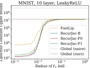
MNIST, 10 layer, LeakyReLU

FastLip RecurJac-B RecurJac-F0 RecurJac-F1 Global (naive) Global (ours)

Figure 1: RecurJac can obtain local and global Lipschitz constants magnitudes better than existing algorithms.

Related Work

Computing Lipschitz constant. Computing a local or global Lipschitz constant of neural networks is a special case of our problem. One simple approach for estimating the Lip-schitz constant for any black-box function is to sample many

x, yand compute the maximal}fpxq´fpyq}{}x´y}(Wood and Zhang 1996). However, the computed value may be an under-estimation unless the sample size goes to infinity. The Extreme Value Theory (De Haan and Ferreira 2007) can be used to refine the bound but the computed value could still under-estimate the Lipschitz constant (Weng et al. 2018b), especially due to the high dimensionality of inputs.

For a neural network with known structure and weights, it is possible to compute Lipschitz constant explicitly. An easy way to obtain a loose global Lipschitz constant is to multiply weight matrices’ operator norms and the maxi-mum derivative of each activation function. Since this quan-tity is simple to compute and can be optimized by back-propagation, many recent works also propose defenses to adversarial examples (Cisse et al. 2017; Elsayed et al. 2018; Tsuzuku, Sato, and Sugiyama 2018; Qian and Wegman 2018) or techniques to improve the training stability of GAN (Miyato et al. 2018) by regularizing this global Lip-schitz constant. However, it is clearly a very loose LipLip-schitz constant, as will be shown in our experiments.

For 2-layer ReLU networks, (Raghunathan, Steinhardt, and Liang 2018) computes a global Lipschitz constant by relaxing the problem to semi-definite programming (SDP) and solving its dual, but it is computationally expensive. For 2-layer networks with twice differentiable activation func-tions, (Hein and Andriushchenko 2017) derives the local Lipschitz constant for robustness verification. These meth-ods show promising results for 2-layer networks, but cannot be trivially extended to networks with multiple layers.

Bounds for Jacobian matrix. Recently, (Weng et al. 2018a) proposes an layer-by-layer algorithm, Fast-Lip, for computing the lower and upper bounds of Jacobian matrix with respect to network inputx. It exploits the special acti-vation patterns in ReLU networks but does not apply to net-works with general activation functions. Most importantly, it

loses power quickly when the network becomes deeper. Us-ing Fast-Lip for robustness verification produces non-trivial bounds only for very shallow networks (less than 4 layers).

Robustness verification of neural networks. Assuming the output of a multi-class classification network fpxqis a

K-dimensional vector where eachfjpxqis the logit for the

j-th class and the final predictionFpxq “arg maxjfjpxq,

the following lemma gives a robustness lower bound (Hein and Andriushchenko 2017; Weng et al. 2018b):

Lemma 1. For an input examplex,

Fpx`∆q “y for all}∆} ămin R,min

j‰y

fypxq ´fjpxq

Lj (

,

(1) whereLjis the Lipschitz constant offjpxq ´fypxqin some

local region (will be formally defined later).

Therefore, as long as a local Lipschitz constant can be computed, we can verify that the prediction of a neural net-work will stay unchanged for any perturbation within radius

R. A good local Lipschitz constant is hard to compute in general: (Hein and Andriushchenko 2017) only shows the results for 2-layer neural networks; (Weng et al. 2018b) ap-plies a sampling-based approach and cannot guarantee that the computed radius satisfies (1). Thus, an efficient, guaran-teed and tight bound for Lipschitz constant is essential for understanding the robustness of deep neural networks.

Other methods have also been proposed for robustness verification, including direct linear bounds (Zhang et al. 2018a; Croce, Andriushchenko, and Hein 2018; Weng et al. 2018a), convex adversarial polytope (Wong and Kolter 2018; Wong et al. 2018), Lagrangian relaxation (Dvijotham et al. 2018) and geometry abstraction (Gehr et al. 2018; Mirman, Gehr, and Vechev 2018). In this paper we focus on Local Lipschitz constant based methods only.

RecurJac: Recursive Jacobian Bounding

In this section, we present RecurJac, our recursive algorithm for uniformly bounding (local) Jacobian matrix of neural networks with a wide range of activation functions.

Notations. For anH-layer neural networkfpxqwith input

xPRn0_{, weight matricesW}plq_P

Rnlˆnl´1_{and bias vectors} bplq _P

Rnl_{, the networkfpxqcan be defined recursively as} hplq_{pxq “σ}plq_pWplq_hpl´1q_pxq`bplq_{qfor alllP t1, . . . , H´}

1uwithhp0q_{:“x,fpxq “W}pHq_hpH´1q_{pxq `b}pHq_.σplq_is a component-wise activation function of (leaky-)ReLU, sig-moid family (including sigsig-moid, arctan, hyperbolic tangent, etc), and other activation functions that satisfy the assump-tions we will formally show below. We denoteWpr,lq: as the

r-th row andWp_:,jlqas thej-th column ofWplq_{. For} conve-nience, we denote fplq_{pxq :“ W}plq_hpl´1q_{pxq `b}plq_{as the} pre-activation function values.

Local Lipchitz constant. Given a functionfpxq:Rn Ñ

Rmand two distance metricsdandd1 onRn andRm,

ball of radiusRcentered ats(denoted asS “Bdrs;Rs) is

defined as:

d1

pfpxq, fpyqq ďLS_d,d1dpx, yq,for allx, yPS:“Bdrs;Rs

Any scalarLS_d,d1that satisfies this condition is a local

Lip-schitz constant. A good local LipLip-schitz constant should be as small as possible,i.e., close tothe best(smallest) local Lips-chitz constant. A LipsLips-chitz constant we compute can be seen as an upper bound of the best Lipschitz constant.

Assumptions on activation functions. RecurJac has the following assumptions on the activation functionσpxq: Assumption 1. σpxqis continuous and differentiable almost everywhere onR. This is a basic assumption for neural

net-work activation functions.

Assumption 2. There exists a positive constantCsuch that

0 ď σ1_{pxq ď C when the derivative exists. This covers} all common activation functions, including (leaky-)ReLU, hard-sigmoid, exponential linear units (ELU), sigmoid, tanh, arctan and all sigmoid-shaped family activation functions. This assumption helps us derive an elegant bound.

Overview of Techniques. The local Lipschitz constant can be presented as the maximum directional derivative in-side the ballBdrs;Rs(Weng et al. 2018b). For differentiable

functions, this is the maximum norm of gradient with respect to the distance metric d(or the maximal operator norm of Jacobian induced by distancesd1_{anddin the vector-output} case). We bound each element of Jacobian through a layer-by-layer approach, as shown below.

Define diagonal matricesΣrepresenting the derivatives of the activation functions:

Σplq_:

“diagtσ1 pfplq

pxqqu.

The Jacobian matrix of aH-layer network can be written as:

∇fpHq

pxq “WpHq_ΣpH´1q_WpH´1q

¨ ¨ ¨Wp2q_Σp1q_Wp1q_. (2) For the ease of notation, we also define

Yp´lq:“ Bf pHq Bhpl´1q “W

pHq_ΣpH´1q

¨ ¨ ¨Wpl`1qΣplqWplq

forlP rHs. As a special case,Yp´1q_:“∇fpHq_.

In the first step, we assume that we have the following pre-activation boundslprlqandurplqfor every layerlP rH´1s:

lplq

r ďfp lq

r pxq ďup lq

r @rP rnls, xPBdrs;Rs (3)

We can get these bounds efficiently via any algo-rithms that compute layer-wise activation bounds, including CROWN (Zhang et al. 2018a) and convex adversarial poly-tope (Wong and Kolter 2018). Because pre-activations are within some ranges rather than fixed values,Σmatrices con-tain uncercon-tainties, which will be characterized analytically.

In the second step, we compute both lower and upper

bounds for each entry of Yp´lq _:“ BfpHq

Bhpl´1q in a

back-ward manner. More specifically, we computeLp´lq_,Up´lq_P

RnHˆnl´1_{so that}

Lp´lqďYp´lqpxq ďUp´lq @xPBdrs;Rs (4)

holds true element-wisely. For layerH, we haveYp´Hq_“ WpHq _{and thus L}p´Hq _{“ U}p´Hq _{“ W}pHq_{. For layers}

l ă H, uncertainties in Σ matrices propagate intoYp´lq layer by layer. Naively deriving pLp´l`1q<sub>,U</sub>p´l`1q

q just from pLp´lq_,Up´lq_{q and pl}pl´1q_,upl´1q_{q leads to a very} loose bound. We propose a fast recursive algorithm that makes use of bounds for all previous layers to compute a much tighter bound for Yp´lq_{. Applying our algorithm} toYp´H`1q<sub>,Y</sub>p´H`2q_{,¨ ¨ ¨ will eventually allow us to} ob-tainYp´1q_{. Our algorithm can also be applied in a forward} manner; the forward version (RecurJac-F) typically leads to slightly tighter bounds but can slow down the computation significantly, as we will show in the experiments.

From an optimization perspective, we essentially try to solve two constrained maximization and minimization prob-lems with variablesΣpr,rlq, for each elementtj, kuin the

Ja-cobian∇fpHq_pxq:

max lrplqďΣr,rplqďuprlq

r∇fpHq_pxqs

j,k and min

lrplqďΣr,rplqďuprlq

r∇fpHq_pxqs j,k.

(5)

Raghunathan, Steinhardt, and Liang (2018) show that even for ReLU networks with one hidden layer, finding the maximum `1 norm of the gradient is equivalent to the

Max-Cut problem and NP-complete. RecurJac is a poly-nomial time algorithm to give upper and lower bounds on r∇fpHqpxqsj,k, rather than solving the exact maxima and

minima in exponential time.

After obtaining the Jacobian bounds Yp´1q _{:“ ∇f}pHq_, we can make use of it to derive an upper bound for the lo-cal Lipchitiz constant in the setS “ Bdrs;Rs. We present

bounds when d and d1 _{are both ordinary p-norm (p “} r1,`8q Y t`8u) distance in Euclidean space. We can also use the Jacobian bounds for other proposes, like understand-ing the local optimization landscape.

Bounds for

Σ

From (2), we can see that the uncertainties in ∇fpHq _are purely fromσ1_pfplq_{pxqq; allW}plq_{are fixed. For anylP rH´}

1s, we define the range ofσ1_pfplq

r pxqqaslr1plqandu1prlq, i.e.,

l1plq

r ďσ1pfp lq

r pxqq ďu1p lq

r @rP rnls. (6)

Note thatl1prlqandu1prlq can be easily obtained because we

knowlprlqďfp lq

r pxq ďup lq

r (thanks to (3)) and the analytical

form ofσ1_{pxq. For example, for the sigmoid functionσpxq “}

ex

1`ex,σ1pxq “σpxqp1´σpxqq, we have:

l1plq

r “

$

’ &

’ % σ1

plrplqq iflp lq

r ďup lq

r ď0;

σ1_puplq

r q ifuprlqělprlqě0;

σ1_pmaxt´lplq

r ,uprlquq iflrplqď0ďuprlq.

(7)

u1plq

r “

$

’ &

’ %

σ1_puplq

r q iflprlqďuprlqď0;

σ1_plplq

r q ifup lq

r ělp lq

r ě0;

σ1_{p0q ifl}plq

r ď0ďup lq

r .

Equations (7) and (8) are also valid for other sigmoid-family activation functions, includingσpxq “ _1`ex_ex,σpxq “ tanhpxq,σpxq “arctanpxqand many others.

For (leaky-)ReLU activation functions with a negative-side slopeα(0ďαď1),lr1plqandu1p

lq

r are:

l1plq

r “

#

α iflprlqďup lq

r ď0 or lp lq

r ď0ďup lq

r ;

1 ifuprlqělprlqě0.

u1plq

r “

#

α iflrplqďup lq

r ď0;

1 ifuprlqělrplqě0 or lprlqď0ďuprlq.

For (leaky-)ReLU activation functions, in the cases where

lprlqďup

lq

r ď0andup lq

r ělp lq

r ě0, we havel1p lq

r “u1p lq

r ,

soΣpr,rlq becomes a constant and there is no uncertainty.

A recursive algorithm to bound

Y

Bounds forYp´H`1q<sub>. By definition, we haveY</sub>p´Hq <sub>“</sub> WpHq<sub>andY</sub>p´H`1q

“Yp´Hq_ΣpH´1q_WpH´1q_{. Thus,}

Yp´_j,kH`1q“ ÿ

rPrnH´1s

W_j,rpHqσ1_pfpH´1q

r qW

pH´1q

r,k , (9)

wherelr1pH´1qďσ1pfp H´1q

r q ďu1p

H´1q

r thanks to (6).

By assumption 2,σ1_{pxqis always non-negative, and thus} we only need to consider the signs ofWpHq_andWpH´1q_. Denote Lp´_j,kH`1q and Up´<sub>j,k</sub>H`1q to be a lower and upper bounds of (9). By examining the signs of each term, we have

Lp´_j,kH`1q“ ÿ

Wp_j,rHqWp_r,kH´1qă0

u1pH´1q

r W

pHq

j,r W

pH´1q

r,k

` ÿ

W_j,rpHqWp_r,kH´1qą0

l1prH´1qW

pHq

j,r W

pH´1q

r,k ,

(10)

Up´_j,kH`1q“ ÿ

W_j,rpHqWp_r,kH´1qą0

u1pH´1q

r W

pHq

j,r W

pH´1q

r,k

` ÿ

Wp_j,rHqWp_r,kH´1qă0

l1pH´1q

r W

pHq

j,r W

pH´1q

r,k .

(11)

In (10), we collect all negative terms of Wp_j,rHqWp_r,kH´1q and multiply them by u1prH´1q as a lower bound of

ř

Wp_j,rHqWp_r,kH´1qă0

σ1_pfpH´1q

r pxqqW_j,rpHqWp_r,kH´1q, and collect

all positive terms and multiply them byl1prH´1qas a lower

bound of the positive counterpart. We obtain the upper bound in (11) following the same rationale. Fast-Lip is a spe-cial case of RecurJac when there are only two layers with ReLU activations; RecurJac becomes much more sophisti-cated in multi-layer cases, as we will show below.

Bounds forYp´lq_{when1 ďl ăH ´1. By definition,} we haveYp´l`1q_“Yp´lq_Σpl´1q_Wpl´1q_{, i.e.,}

Yp´_j,kl`1q“ ÿ

rPrnl´1s

Yp´_j,rlqσ1 pfpl´1q

r pxqqW

pl´1q

r,k , (12)

wherel1prl´1qďσ1pfrpl´1qpxqq ďu1prl´1qthanks to (6) and

L_j,rp´lqďY_j,rp´lqďUp´_j,rlq @j, r

thanks to previous computation. We want to find the bounds

L_j,kp´l`1qďY<sub>j,k</sub>p´l`1qďUp´_j,kl`1q @j, k.

We decompose (12) into two terms:

Yp´_j,kl`1q“ ÿ tr:Lp´_j,rlqă0ăUp´_j,rlqu

Yp´_j,rlqσ1_pfpl´1q

r pxqqW

pl´1q

r,k

loooooooooooooooooooooooooooomoooooooooooooooooooooooooooon

I

` ÿ

tr:Lp´_j,rlqě0orUp´_j,rlqď0u

Yp´_j,rlqσ1 pfpl´1q

r pxqqW

pl´1q

r,k

loooooooooooooooooooooooooooooomoooooooooooooooooooooooooooooon

II

,

(13) and bound them separately.

Observing the signs of each term in I and u1prl`1q ě lr1pl`1qě0, we take:

Lp´_j,kl`1q,˘“ ÿ

Wp_r,kl´1qă0

u1prl´1qUp´j,rlqW pl´1q r,k `

ÿ

Wp_r,kl´1qą0

u1prl´1qLp´j,rlqW pl´1q r,k

(14)

Up´_j,kl`1q,˘“ ÿ

Wp_r,kl´1qă0

u1prl´1qLp´j,rlqW pl´1q r,k `

ÿ

Wp_r,kl´1qą0

u1prl´1qUp´j,rlqW pl´1q r,k

(15)

The index constrainttr : Lp´_j,rlq ă 0 ă Up´_j,rlquis still effective in (14) and (15), but we omit it for notation sim-plicity. Then we can show thatLp´_j,kl`1q,˘andUp<sub>j,k</sub>l`1q,˘are a lower and upper bound for termIin (13) as follows. Proposition 1.

Lp´_j,kl`1q,˘ďIďUp´<sub>j,k</sub>l`1q,˘, (16) whereIis the first term in(13).

For term II in (13), the sign of Yp´_j,rlq does not change since Lp´_j,rlq ě 0 or Up´_j,rlq ď 0. Similar to what we did in (10) and (11), depending on the sign of Yp´_j,rlqWp_r,kl´1q, we can lower/upper bound term II using Yp´lq _itself in-stead of its bound pLp´lq_,Up´lq_{q. This will give us much} tighter bounds than just naively usingpLp´lq_,Up´lq_{qas we} deal with termI. More specifically, we define2nHmatrices

|

Wpl,l´1,jq_,

x

Wpl,l´1,jq_P

Rnlˆnl´2_{forjP rn}

Hsas below:

|

W_i,kpl,l´1,jq“ ÿ

Lp´_j,rlqě0,Wp_r,kl´1qą0

orUp´_j,rlqď0,W_r,kpl´1qă0

Wp_i,rlql1prl´1qW

pl´1q

r,k

` ÿ

Lp´_j,rlqě0,Wp_r,kl´1qă0

orUp´_j,rlqď0,Wp_r,kl´1qą0

Wp_i,rlqu1pl´1q

r W

pl´1q

r,k ,

x

W_i,kpl,l´1,jq“ ÿ

Lp´_j,rlqě0,Wp_r,kl´1qą0

orUp´_j,rlqď0,W_r,kpl´1qă0

Wp_i,rlqu1pl´1q

r W

pl´1q

r,k

` ÿ

Lp´_j,rlqě0,Wp_r,kl´1qă0

orUp´_j,rlqď0,Wp_r,kl´1qą0

Wp_i,rlql1pl´1q

r W

pl´1q

r,k .

(18)

Then we can show the following lemma. Lemma 2. For anyjP rnHs, we have

Y_j,p´_:l´1qΣplqW|p l,l´1,jq

:,k ďII ďY

p´l´1q

j,: Σ

plq

x

Wp_:,kl,l´1,jq,

(19) whereIIis the second term in(13).

Note that when the sign ofY_j,rp´lq is fixed, i.e.,Lp´_j,rlq ě

0 or Up´_j,rlq ď 0 in term II, the bounds in (19) is always tighter than those in (16). After we know the sign of Yp´_j,rlq, we can fix σ1_pfpl´1q

r pxqq to be either

l1prl´1q or u1p

l´1q

r according to the sign of Wp l´1q

r,k and

thus eliminate the uncertainty in σ1_pfpl´1q

r pxqq. Then we

can plug Yp´_j,rlq “ ř_sY_j,ip´l´1qσ1_pfplq

i pxqqW

plq

i,r into the

lower and upper bounds and merge terms involvingWp_i,rlq,

σ1_pfpl´1q

r pxqqandWp l´1q

r,k , resulting in (19). Compared with

using the worst-case bound Lp´_j,rlq ď Y_j,rp´lq ď Up´_j,rlq di-rectly in (16), we expandYp´_j,rlqand remove uncertainty in

σ1_pfpl´1q

r pxqqin (19), and thus get much tighter bounds.

Finally, combining Proposition 1 and Lemma 2, we get the following recursive formula to boundYp´l`1q_.

Theorem 1. For any1ălăHand anyjP rnHs, we have

Y_j,p´_:l`1qěLp´<sub>j,:</sub>l`1q,˘`Y_j,p´_:l´1qΣplq

|

Wp_:,kl,l´1,jq

and

Yp´_j,:l`1qďUp´<sub>j,:</sub>l`1q,˘`Yp´_j,:l´1qΣplq

x

Wp_:,kl,l´1,jq,

whereLp´l`1q,˘<sub>,U</sub>p´l`1q,˘_,

|

Wpl,l´1,jq_and

x

Wpl,l´1,jq_are defined in(14),(15),(17)and(18), respectively.

Remark 1. The lower and upper bounds of Yp´H`1q _in (10) and (11) can be viewed as a special case of Theo-rem 1 whenl “H. Because we haveLp´Hq _“Up´Hq _“ Wplq _{in this case, we do not have term I in the} de-composition (13). Moreover, the bounds of term II in (19) are reduced to exactly (10) and (11) after we no-tice that W|p

H,H´1,jq

j,k “ L

p´H`1q

j,k and Wx

pH,H´1,jq

j,k “

Up´_j,kH`1qand specifyYp´H´1q_“ΣpHq_“I

nH. Specifying

Yp´H´1q _{“ Σ}pHq _{“ I}

nH is equivalent to adding another

identity layer to the neural networkfpHq_pxq.

A recursive algorithm to bound Yp´lq_{. Notice that the} lower and upper bounds in Lemma 2 have exactly the same formation ofYp´lq_“Yp´l´1q_Σplq_Wplq_{, by replacingW}plq

with W|pl,l´1,jq andWxpl,l´1,jq. Therefore, we can

recur-sively apply our Theorem 1 to obtain an lower and upper bound forYp´l`1q<sub>, denoted asL</sub>p´l`1q_andUp´l`1q sepa-rately. This recursive procedure further reduces uncertainty inΣfor all previous layers, improving the quality of bounds significantly. We elaborate our recursive algorithm in Algo-rithm 1 for the casenH“1, so we omit the last superscript

j “1inW|pl,l´1,1qandWxpl,l´1,1q. WhennH ą1, we can

apply Algorithm 1 independently for each output.

Algorithm 1ComputeLU (compute the lower and upper Ja-cobian bounds)

Require: Wplq_{, bounds tpL}p´iq_,Up´iq_,Wpiq_quH i“l`1,

tl1pi´1q_,u1pi´1q_uH i“l`1

1: ifl“H then

2: Lp´lq_“Up´lq_“Wplq 3: else ifl“H´1then

4: ComputeLp´lq_{from (10),U}p´lq_{from (11)} 5: else if1ďlăH´1then

6: ComputeW|pl`1,lqfrom (17),Wxpl`1,lqfrom (18)

7: pLp´l´1,´lq_{,vq = ComputeLU( W|}pl`1,lq_, tpLp´iq_,Up´iq_,Wpiq_quH

i“l`2, tl1p

i´1q_,u1pi´1q_uH i“l`2)

8: p_v,Up´l´1,´lq_{q = ComputeLU(}

x

Wpl`1,lq_, tpLp´iq_,Up´iq_,Wpiq_quH

i“l`2, tl1p

i´1q_,u1pi´1q_uH i“l`2)

9: ComputeLp´lq,˘_{from (14),U}p´lq,˘_{from (15)} 10: Lp´lq_“Lp´lq,˘_`Lp´l´1,´lq

11: Up´lq_“Up´lq,˘_`Up´l´1,´lq 12: end if

13: returnLp´lq_,Up´lq

Compute the bounds in a forward manner. In previous sections, we start our computation from the last layer and

bound Yp´lq _:“ BfpHq

Bhpl´1q in a backward manner. By

trans-posing (2), we have

r∇fpHqpxqsT “Wp1qT_Σp1q_Wp2qT

¨ ¨ ¨ΣpH´1q_WpHqT_.

Then we can apply Algorithm 1 to bound ∇fpHq_pxqT

ac-cording to the equation above. This is equivalent to starting

from the first layer, and bound Bf_Bp_xlq froml “1toH. Be-cause we obtain the bounds of pre-activations in a forward manner by CROWN (Zhang et al. 2018a), the bounds (3) get looser when the layer indexlgets larger. Therefore, bound-ing the Jacobian by the forward version is expected to get

tighter bounds of Bf_Bxplq at least for small l. In our experi-ments, we see that the bounds for∇fpHq_{pxqobtained from} the forward version are typically a little tighter than those obtained from the backward version. However, the “output” dimension in this case isn0, which is the input dimension

of the neural network. For image classification networks,

nH ! n0, the forward version has to apply Algorithm 1

n0 times to obtain the final bounds and thus increases the

Compute a local Lipschitz constant

ďYp´1q_:

“∇fpxq ďUp´1q_{for all}

xPS, we define

max

xPS |r∇fpxqs| ďM:“maxp|L

p´1q

|,|Up´1q|q, (20)

where the max and inequality are taken element-wise. In the rest of this subsection, we simplify the notations Yp´1q_,Lp´1q_,Up´1q_{toY,L,Uwhen no confusion arises.}

Recall that the Local Lipschitz constantLS

d can be

eval-uated asLS

d,d1 “ maxxPS}∇fpxq}d,d1.∇fpxqis the

Jaco-bian matrix and} ¨ }d,d1denotes the induced operator norm.

Then we can bound the maximum norm of Jacobian (local Lipschitz constant) considering its element-wise worst case. Whend,d1_{are both ordinaryp-norm (p“ r1,`8qYt`8u)} distance in Euclidean space, we denoteLd,d1 asL_p, and it

can be bounded as follows.

Proposition 2. For any1ďpď `8, we have

LS_p :“ max

xPB`prs;Rs

}∇fpxq}pď }M}p, (21)

whereM:“maxp|L|,|U|qis defined in(20).

Improve the bound forLS

8. For the important case of up-per boundingLS₈, we use an additional trick to improve the bound (21). We note that}∇fpxq}8“maxjř_k|Yj,k|. As

in (13), we decompose it into two terms

ÿ

k

|Y_j,k| “ ÿ

kPTj

|Y_j,k|

loooomoooon

I

` ÿ

kPT` j

Y_j,k´ ÿ

kPT´ j

Y_j,k

looooooooooooomooooooooooooon

II

, (22)

whereT`

j :“ tk|Lj,k ě 0u, Tj´ :“ tk|Uj,k ď 0u, and

Tj :“ tk|Lj,kă0ăUj,ku.

For termI, we take the same bound as we have in (21), i.e.,Iďř_kPT

jMj,k.

For termII, thanks toY “Yp´2q_Σp1q_Wp1q_{, we have}

II “ÿ

r

Y_j,rp´2qσ1_pfp1q

r pxqqp ÿ

kPT` j

Wp_r,k1q´ ÿ

kPT´ j

Wp_r,k1qq.

Definew_ppjq_P

Rn1ˆ1_and

p wpjq

r :“ ÿ

kPT` j

W_r,kp1q´ ÿ

kPT´ j

Wp_r,k1q. (23)

Algorithm 2Upper bound ofmaxxPB`8rs;Rs}∇fpxq}8

1: ComputeMfrom (20) 2: forjP rnHsdo

3: Computew_pprjqfrom (23)

4: p_v,Up0,jq_{q = ComputeLU(}

p wprjq,

tpLp´iq_,Up´iq_,Wpiq_quH

i“1,tl1pi´1q, u1pi´1quHi“1)

5: Up_j0q“Up0,jq_`ř

kPTjMj,k

6: end for

7: returnmaxjPrnHsU p0q

j

Combining upper bounds for both terms, we obtain

ÿ

j

|Yi,j| ď ÿ

kPTj

Mj,k`Y

p´2q

j,: Σ

p1q

p wpjq

In the same flavor with Theorem 1, this bound avoids the worst case boundM_j,k for entries whose signs are known.

Notice thatYp´_j,:2qΣp1q

p

wpjq_{has exactly the same formation} ofYp´1q_{and we can call Algorithm 1 to get its upper bound.} Finally, assume that from Algorithm 1 we already ob-tainedtpLp´lq_,Up´lq

quHl“1, we summarize the algorithm to

compute upper bound ofLS

8in Algorithm 2.

Improve the bound for robustness verification. In some applications (e.g., robustness verification), we only need to bound}fpxq´fpsq}for a fixedsandxPBrs;Rs. Although

LBrs;Rs_{¨Rgives a bound of}fpxq ´fpsq}, we can make} this bound tighter by using an integral:

Theorem 2.

}fpxq´fpsq} ď

żR

0

LBrs;ts_dt

ďLBrs;Rs

¨R,@xPBrs;Rs.

In practice, the integral şR₀ LBrs;ts_{dt can be upper} bounded by evaluating atnintervals:

żR

0

LBrs;ts_dt ď

n ÿ

i“1

LBrs;tis_{∆t, (24)}

where we divide R into n segments t0 “

0, t1, t2,¨ ¨ ¨, tn´1, tn“R, andti`1´ti“∆t.

Applications and Experiments

2 4 6 8 10

Network depth

0.00 0.25 0.50 0.75 1.00 1.25 1.50

R

ad

iu

s

of

ℓ2

b

al

l,

R

* 2

ℓ2

0.00 0.02 0.04 0.06 0.08 0.10

R

ad

iu

s

of

ℓ∞

b

al

l,

R

* ∞

MNIST, 2-10 layers, LeakyReLU

ℓ∞

Figure 2: The largest radiusR˚_{within which no stationary} point exists, for network with different depths (2-10 layers)

Local optimization landscape. In non-convex optimiza-tion, a zero gradient vector results in a stationary point, po-tentially a saddle point or a local minimum. The existence of saddle points and local minima is one of the main diffi-culties for non-convex optimization (Dauphin et al. 2014),

1

10−3 ₁₀−2 ₁₀−1 ₁₀0 Radius of ℓ∞ ball

103 104 105

Lipschitz Constant Upper Bound

MNIST, 5 layer, tanh

RecurJac-B RecurJac-F0 RecurJac-F1 Global (naive) Global (ours)

(a) MNIST 5-layertanhactivation

10−3 ₁₀−2 ₁₀−1 ₁₀0

Radius of ℓ∞ ball

102 103 104 105 106 107

Lipschitz Constant Upper Bound

MNIST, 7 layer, ReLU

FastLip RecurJac-B RecurJac-F0 RecurJac-F1 Global (naive) Global (ours)

(b) MNIST 7-layer ReLU activation

10−3 ₁₀−2 ₁₀−1 ₁₀0

Radius of ℓ∞ ball

104

106

108

1010

1012

Lipschitz Constant Upper Bound

CIFAR, 10 layer, ReLU

FastLip RecurJac-B RecurJac-F0 RecurJac-F1 Global (naive) Global (ours)

(c) CIFAR 10-layer ReLU activation

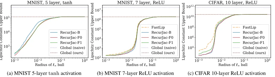
Figure 3: Global and local Lipschitz constants on three networks. FastLip can only be applied to (leaky)ReLU networks.

runner-up target random target least-likely target Network Method Undefended Adv. Training Undefended Adv. Training Undefended Adv. Training

MNIST 3-layer

RecurJac 0.02256 0.11573 0.02870 0.13753 0.03205 0.16153

FastLip 0.01802 0.09639 0.02374 0.11753 0.02720 0.14067 MNIST

4-layer

RecurJac 0.02104 0.07350 0.02399 0.08603 0.02519 0.09863

FastLip 0.01602 0.04232 0.01882 0.05267 0.02018 0.06417

Table 1: Comparison of the lower bounds for`8 distortion found by RecurJac (our algorithm) and FastLip on models with adversarial training with PGD perturbation“0.3for two models and 3 targeted attack classes, averaged over 100 images.

including optimization problems on neural networks. How-ever, if for at least one pair oftj, kuwe haveU_j,k ă0or L_j,k ą0, the JacobianY will never become a zero matrix within a local region.

In this experiment, we train an MLP network with leaky-ReLU activation (α“0.3) for MNIST and varying network depth from 2 to 10. Each hidden layer has 20 neurons, and all models achieve over 96% accuracy on validation set. We randomly choose 500 images of digit “1” from the test set that are correctly classified by all models, and bound the gradient off1pxq(logit output for class “1”). For each

im-age, we record the largest`2and`8 distortion (denoted as

R˚

2 andR˚8) added such that there is at least one element

k in∇f1pxqthat can never reach zero (i.e.,U1,k ă 0 or

L_1,ką0). The reportedR˚_{are the average of 500 images.} Figure 2 shows howR˚ _{decreases as the network depth} increases. Interestingly, for the smallest network with only 2 layers, no stationary point is found in its entire domain (R˚ _{“ 8). For deeper networks, the region without} sta-tionary points nearxbecomes smaller, indicating the diffi-culty of finding optimal adversarial examples (a global op-tima with minimum distortion) grows with network depth.

Local and global Lipschitz constant. We apply RecurJac to get local and global Lipschitz constants on 4 networks of different scales for MNIST and CIFAR. For MNIST, we use a 10-layer leaky-ReLU network with 20 neurons per layer, a 5-layertanhnetwork with 50 neurons per layer, a 7-layer ReLU network with 1024, 512, 256, 128, 64 and 32 hidden neurons; for CIFAR, we use a 10-layer network with 2048, 2048, 1024, 1024, 512, 512, 256, 256, 128 hidden neurons.

As a comparison, we include Lipschitz constants com-puted by Fast-Lip (Weng et al. 2018a), a state-of-the-art

al-gorithm for ReLU networks (we also trivially extended it to the leaky ReLU case for comparison). For our algorithm, we run both the backward and the forward versions, de-noted as RecurJac-B (Algorithm 1) and RecurJac-F0 (the forward version). RecurJac-F0 requires to maintain inter-mediate bounds in shape nlˆn0, thus the computational

cost is very high. We implemented another forward version, RecurJac-F1, which starts intermediate bounds after the first layer and reduce the space complexity tonlˆn1.

We randomly select an image for each dataset and as the input. Then, we upper bound the Local Lipschitz constant within an `8 ball of radius R. As shown in Figure 1 and 3, for all networks, whenRis small, our algorithms signif-icantly outperforms Fast-Lip as we find much smaller (and thus in better quality) Lipschitz constants (sometimes a few magnitudes smaller, noting the logarithmic y-axis); WhenR

is large, local Lipschitz constant converges to a value which corresponds to the worst case activation pattern, which is in fact a global Lipschitz constant. Although this value is large, it is still magnitudes smaller than the global Lipschitz constant obtained by the naive product of weight matrices’ induced norms (dotted lines with label “naive”).

For the largest CIFAR network, the average computation time for 1 local Lipschitz constant of FastLin, RecurJac-B, RecurJac-F0 and RecurJac-F1 are 2.4 sec, 10.5 sec, 1 hr and 5 hr respectively, on 1 CPU core. RecurJac-F0 and RecurJac-F1 sometimes provide better results than RecurJac-B (Fig. 3a). However whennH !n0, RecurJac-B

is preferred due to its computational efficiency.

Robustness verification for adversarial examples. For a correctly classified source imagesof classcand an attack target classj, we definegpsq “fcpsq ´fjpsq ą0that

if gpxq goes below 0, an adversarial example xis found. Using Theorem 2, we know that the largest R such that

şR

0 L

Brs;ts_{pgqdtăgpsqis a certified robustness lower bound} within which no adversarial examples of class j can be found. In this experiment, we approximate the integral in (24) from above by using 30 intervals.

We evaluate the robustness lower bound on unde-fended networks and adversarially trained networks pro-posed by (Madry et al. 2018). We use two MLP networks with 3 and 4 layers with 1024 neurons per layer. Table 1 shows that our algorithm can indeed reflect the increased robustness as the certified lower bounds under “Adv. Train-ing” column become much larger than “Undefended”. Addi-tionally, when the adversarial training procedure attempts to defend against adversarial examples with`8 distortion less than 0.3, our bounds are better than Fast-Lip and closer to 0.3, suggesting that adversarial training is effective.

Conclusion

In this paper, we propose a novel algorithm, RecurJac, for re-cursively bounding a neural network’s Jacobian matrix with respect to its input. Our method can be efficiently applied to networks with a wide class of activation functions. Applica-tions of RecurJac include characterizing local optimization landscape, computing a local or global Lipschitz constant, and robustness verification of neural networks.

References

Arjovsky, M.; Chintala, S.; and Bottou, L. 2017. Wasserstein generative adversarial networks. InICML, 214–223. Arora, S., and Zhang, Y. 2018. Do GANs actually learn the distribution? an empirical study. ICLR.

Bartlett, P. L.; Foster, D. J.; and Telgarsky, M. J. 2017. Spectrally-normalized margin bounds for neural networks. InNIPS, 6240–6249.

Cisse, M.; Bojanowski, P.; Grave, E.; Dauphin, Y.; and Usunier, N. 2017. Parseval networks: Improving robustness to adversarial examples. ICML.

Croce, F.; Andriushchenko, M.; and Hein, M. 2018. Prov-able robustness of ReLU networks via maximization of lin-ear regions. arXiv preprint arXiv:1810.07481.

Dauphin, Y. N.; Pascanu, R.; Gulcehre, C.; Cho, K.; Gan-guli, S.; and Bengio, Y. 2014. Identifying and attacking the saddle point problem in high-dimensional non-convex opti-mization. InNIPS, 2933–2941.

De Haan, L., and Ferreira, A. 2007. Extreme value theory: an introduction. Springer Science & Business Media. Dvijotham, K.; Stanforth, R.; Gowal, S.; Mann, T.; and Kohli, P. 2018. A dual approach to scalable verification of deep networks.UAI.

Elsayed, G. F.; Krishnan, D.; Mobahi, H.; Regan, K.; and Bengio, S. 2018. Large margin deep networks for classifi-cation. arXiv preprint arXiv:1803.05598.

Gehr, T.; Mirman, M.; Drachsler-Cohen, D.; Tsankov, P.; Chaudhuri, S.; and Vechev, M. 2018. AI2: Safety and

robust-ness certification of neural networks with abstract interpre-tation. In2018 IEEE Symposium on Security and Privacy. Goodfellow, I.; Pouget-Abadie, J.; Mirza, M.; Xu, B.; Warde-Farley, D.; Ozair, S.; Courville, A.; and Bengio, Y. 2014. Generative adversarial nets. InNIPS, 2672–2680. Gulrajani, I.; Ahmed, F.; Arjovsky, M.; Dumoulin, V.; and Courville, A. 2017. Improved training of Wasserstein GANs. NIPS.

Hein, M., and Andriushchenko, M. 2017. Formal guarantees on the robustness of a classifier against adversarial manipu-lation. InNIPS, 2266–2276.

Madry, A.; Makelov, A.; Schmidt, L.; Tsipras, D.; and Vladu, A. 2018. Towards deep learning models resistant to adversarial attacks. InICLR.

Mirman, M.; Gehr, T.; and Vechev, M. 2018. Differentiable abstract interpretation for provably robust neural networks. InICML, 3575–3583.

Miyato, T.; Kataoka, T.; Koyama, M.; and Yoshida, Y. 2018. Spectral normalization for generative adversarial networks. arXiv preprint arXiv:1802.05957.

Qian, H., and Wegman, M. N. 2018. L2-nonexpansive neu-ral networks. arXiv preprint arXiv:1802.07896.

Raghunathan, A.; Steinhardt, J.; and Liang, P. 2018. Certi-fied defenses against adversarial examples. ICLR.

Sriperumbudur, B. K.; Fukumizu, K.; Gretton, A.; Sch¨olkopf, B.; and Lanckriet, G. R. 2009. On in-tegral probability metrics,zphi-divergences and binary classification.arXiv preprint arXiv:0901.2698.

Tsuzuku, Y.; Sato, I.; and Sugiyama, M. 2018. Lipschitz-margin training: Scalable certification of perturbation in-variance for deep neural networks. arXiv preprint arXiv:1802.04034.

Vapnik, V. N., and Vapnik, V. 1998. Statistical learning theory, volume 1. Wiley New York.

Weng, T.-W.; Zhang, H.; Chen, H.; Song, Z.; Hsieh, C.-J.; Boning, D.; Dhillon, I. S.; and Daniel, L. 2018a. Towards fast computation of certified robustness for ReLU networks. InInternational Conference on Machine Learning.

Weng, T.-W.; Zhang, H.; Chen, P.-Y.; Yi, J.; Su, D.; Gao, Y.; Hsieh, C.-J.; and Daniel, L. 2018b. Evaluating the robust-ness of neural networks: An extreme value theory approach. ICLR.

Wong, E., and Kolter, Z. 2018. Provable defenses against adversarial examples via the convex outer adversarial poly-tope. InICML, 5283–5292.

Wong, E.; Schmidt, F.; Metzen, J. H.; and Kolter, J. Z. 2018. Scaling provable adversarial defenses. NIPS.

Wood, G., and Zhang, B. 1996. Estimation of the Lips-chitz constant of a function.Journal of Global Optimization 8(1):91–103.

Zhang, H.; Weng, T.-W.; Chen, P.-Y.; Hsieh, C.-J.; and Daniel, L. 2018a. Efficient neural network robustness certi-fication with general activation functions. InNIPS.