MEAL: Multi-Model Ensemble via Adversarial Learning

The Thirty-Third AAAI Conference on Artificial Intelligence (AAAI-19)

MEAL: Multi-Model Ensemble via Adversarial Learning

Zhiqiang Shen,

Zhankui He,

Xiangyang Xue

School of Computer Science, Fudan University, Shanghai, China

2_{Beckman Institute, University of Illinois at Urbana-Champaign, IL, USA} 3_{School of Data Science, Fudan University, Shanghai, China}

[email protected],{zkhe15, xyxue}@fudan.edu.cn

Abstract

Often the best performing deep neural models are ensembles of multiple base-level networks. Unfortunately, the space re-quired to store these many networks, and the time rere-quired to execute them at test-time, prohibits their use in applica-tions where test sets are large (e.g., ImageNet). In this pa-per, we present a method for compressing large, complex trained ensembles into a single network, where knowledge from a variety of trained deep neural networks (DNNs) is distilled and transferred to a single DNN. In order to distill diverse knowledge from different trained (teacher) models, we propose to use adversarial-based learning strategy where we define a block-wise training loss to guide and optimize the predefined student network to recover the knowledge in teacher models, and to promote the discriminator network to distinguish teachervs.student features simultaneously. The proposed ensemble method (MEAL) of transferring distilled knowledge with adversarial learning exhibits three important advantages: (1) the student network that learns the distilled knowledge with discriminators is optimized better than the original model; (2) fast inference is realized by a single for-ward pass, while the performance is even better than tra-ditional ensembles from multi-original models; (3) the stu-dent network can learn the distilled knowledge from a teacher model that has arbitrary structures. Extensive experiments on CIFAR-10/100, SVHN and ImageNet datasets demonstrate the effectiveness of our MEAL method. On ImageNet, our ResNet-50 based MEAL achieves top-1/5 21.79%/5.99% val error, which outperforms the original model by 2.06%/1.14%.

1. Introduction

The ensemble approach is a collection of neural networks whose predictions are combined at test stage by weighted averaging or voting. It has been long observed that en-sembles of multiple networks are generally much more ro-bust and accurate than a single network. This benefit has also been exploited indirectly when training a single net-work through Dropout (Srivastava et al. 2014), Dropcon-nect (Wan et al. 2013), Stochastic Depth (Huang et al. 2016), Swapout (Singh, Hoiem, and Forsyth 2016), etc. We extend this idea by forming ensemble predictions during training,

∗

equal contribution. This work was done when Zhankui He was a research intern at University of Illinois at Urbana-Champaign.

Copyright c2019, Association for the Advancement of Artificial

Intelligence (www.aaai.org). All rights reserved.

1

2

3

4

5

# of ensembles

0×

1×

2×

3×

4×

5×

6×

FLOPs

FLOPs at Inference Time

Snapshot Ensemble

(Huang et al. 2017)

Our FLOPs at Test Time

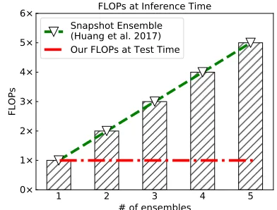
Figure 1: Comparison of FLOPs at inference time. Huang et al. (Huang et al. 2017a) employ models at different lo-cal minimum for ensembling, which enables no additional training cost, but the computational FLOPs at test time lin-early increase with more ensembles. In contrast, our method use only one model during inference time throughout, so the testing cost is independent of # ensembles.

using the outputs of different network architectures with dif-ferent or identical augmented input. Our testing still operates on a single network, but the supervision labels made on dif-ferent trained networks correspond to an ensemble pre-diction of a group of individual reference networks.

The traditional ensemble, or called true ensemble, has some disadvantages that are often overlooked. 1) Redun-dancy: The information or knowledge contained in the trained neural networks are always redundant and has over-laps between with each other. Directly combining the pre-dictions often requires extra computational cost but the gain is limited. 2) Ensemble is always large and slow: Ensem-ble requires more computing operations than an individual network, which makes it unusable for applications with lim-ited memory, storage space, or computational power such as desktop, mobile and even embedded devices, and for appli-cations in which real-time predictions are needed.

library bookshop

confectionery grocery store

tobacco shop toyshop

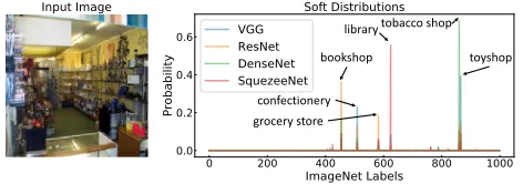
Figure 2: Left is a training example of class “tobacco shop” from ImageNet. Right are soft distributions from different trained architectures. The soft labels are more informative

and can provide more coverage for visually-related scenes.

without incurring any additionaltesting costs. We achieve this goal by leveraging the combination of diverse outputs from different neural networks as supervisions to guide the target network training. The reference networks are called

Teachersand the target networks are calledStudents. Instead

of using the traditional one-hot vector labels, we use thesoft

labels that provide more coverage for co-occurring and visu-ally related objects and scenes. We argue that labels should be informative for the specific image. In other words, the labels should not be identical for all the given images with the same class. More specifically, as shown in Fig. 2, an im-age of “tobacco shop” has similar appearance to “library” should have a different label distribution than an image of “tobacco shop” but is more similar to “grocery store”. It can also be observed that soft labels can provide the additional intra- and inter-category relations of datasets.

To further improve the robustness of student networks, we introduce an adversarial learning strategy to force the student to generate similar outputs as teachers. Our exper-iments show that MEAL consistently improves the accu-racy across a variety of popular network architectures on different datasets. For instance, our shake-shake (Gastaldi 2017) based MEAL achieves 2.54% test error on CIFAR-10, which is a relative11.2%improvement1. On ImageNet, our ResNet-50 based MEAL achieves 21.79%/5.99% val error, which outperforms the baseline by a large margin.

In summary, our contribution in this paper is three fold.

• An end-to-end framework with adversarial learning is de-signed based on theteacher-studentlearning paradigm for deep neural network ensembling.

• The proposed method can achieve the goal of ensembling multiple neural networks with no additionaltesting cost.

• The proposed method improves the state-of-the-art accu-racy on CIFAR-10/100, SVHN, ImageNet for a variety of existing network architectures.

2. Related Work

There is a large body of previous work (Hansen and Salamon 1990; Perrone and Cooper 1995; Krogh and Vedelsby 1995; Dietterich 2000; Huang et al. 2017a; Lakshminarayanan, Pritzel, and Blundell 2017) on ensembles with neural net-works. However, most of these prior studies focus on

im-1

Shake-shake baseline (Gastaldi 2017) is 2.86%.

proving the generalization of an individual network. Re-cently, Snapshot Ensembles (Huang et al. 2017a) is pro-posed to address the cost of training ensembles. In contrast to the Snapshot Ensembles, here we focus on the cost of

test-ing ensembles. Our method is based on the recently raised

knowledge distillation (Hinton, Vinyals, and Dean 2015; Papernot et al. 2017; Li et al. 2017; Yim et al. 2017) and adversarial learning (Goodfellow et al. 2014), so we will re-view the ones that are most directly connected to our work.

“Implicit” Ensembling.Essentially, our method is an “im-plicit” ensemble which usually has high efficiency during both training and testing. The typical “implicit” ensemble methods include: Dropout (Srivastava et al. 2014), Drop-Connection (Wan et al. 2013), Stochastic Depth (Huang et al. 2016), Swapout (Singh, Hoiem, and Forsyth 2016), etc. These methods generally create an exponential number of networks with shared weights during training and then im-plicitly ensemble them at test time. In contrast, our method focuses on the subtle differences of labels with identical in-put. Perhaps the most similar to our work is the recent pro-posed Label Refinery (Bagherinezhad et al. 2018), who fo-cus on the single model refinement using the softened labels from the previous trained neural networks and iteratively learn a new and more accurate network. Our method differs from it in that we introduce adversarial modules to force the model to learn the difference between teachers and students, which can improve model generalization and can be used in conjunction with any other implicit ensembling techniques.

Adversarial Learning. Generative Adversarial Learn-ing (Goodfellow et al. 2014) is proposed to generate realistic-looking images from random noise using neural networks. It consists of two components. One serves as a generator and another one as a discriminator. The gener-ator is used to synthesize images to fool the discrimina-tor, meanwhile, the discriminator tries to distinguish real and fake images. Generally, the generator and discrimina-tor are trained simultaneously through competing with each other. In this work, we employ generators to synthesize stu-dent features and use discriminator to discriminate between teacher and student outputs for the same input image. An advantage of adversarial learning is that the generator tries to produce similar features as a teacher that the discrimi-nator cannot differentiate. This procedure improves the ro-bustness of training for student network and has applied to many fields such as image generation (Johnson, Gupta, and Fei-Fei 2018), detection (Bai et al. 2018), etc.

Knowledge Transfer. Distilling knowledge from trained neural networks and transferring it to another new network has been well explored in (Hinton, Vinyals, and Dean 2015; Chen, Goodfellow, and Shlens 2016; Li et al. 2017; Yim et al. 2017; Bagherinezhad et al. 2018; Anil et al. 2018). The typical way of transferring knowledge is theteacher-student

learning paradigm, which uses a softened distribution of the

pa-Te

ac

h

er

N

Alignment Similarity Loss

Alignment

Discriminator

Teacher Net

Student Net Alignment

Alignment

Discriminator

Alignment Alignment

Discriminator

Similarity Loss Similarity Loss

Generator

Binary Cross-entropy Loss Fc Layers Teacher

Selection Module

…

h

er

A

Figure 3: Overview of our proposed architecture. We input the same image into the teacher and student networks to generate intermediate and final outputs forSimilarity LossandDiscriminators. The model is trained adversarially against several

dis-criminator networks. During training the model observes supervisions from trained teacher networks instead of the one-hot

ground-truth labels, and the teacher’s parameters are fixed all the time.

rameters from two networks. Bagherinezhad et al. (Bagher-inezhad et al. 2018) studied the effects of various properties of labels and introduce theLabel Refinerymethod that iter-atively updated the ground truth labels after examining the entire dataset with the teacher-student learning paradigm.

3. Overview

Siamese-like Network Structure Our framework is a siamese-like architecture that contains two-stream networks in teacher and student branches. The structures of two streams can be identical or different, but should have the same number of blocks, in order to utilize the intermediate outputs. The whole framework of our method is shown in Fig. 3. It consists of a teacher network, a student network, alignment layers, similarity loss layers and discriminators.

The teacher and student networks are processed to gener-ate intermedigener-ate outputs for alignment. The alignment layer is an adaptive pooling process that takes the same or differ-ent length feature vectors as input and output fixed-length new features. We force the model to output similar features of student and teacher by training student network adversar-ially against several discriminators. We will elaborate each of these components in the following sections with more de-tails.

4. Adversarial Learning (AL) for Knowledge

Distillation

4.1 Similarity Measurement

Given a datasetD = (Xi, Yi), we pre-trained the teacher

network Tθ over the dataset using the cross-entropy loss

against the one-hot image-level labels2in advance. The

stu-2

Ground-truth labels

dent network Sθ is trained over the same set of images,

but uses labels generated by Tθ. More formally, we can

view this procedure as trainingSθon a new labeled dataset

˜

D= (Xi,Tθ(Xi)). Once the teacher network is trained, we

freeze its parameters when training the student network. We train the student networkSθ by minimizing the

sim-ilarity distance between its output and the soft label gener-ated by the teacher network. LettingpTθ

c (Xi) =Tθ(Xi)[c],

pSθ

c (Xi) =Sθ(Xi)[c]be the probabilities assigned to classc

in the teacher modelTθand student modelSθ. The similarity

metric can be formulated as:

LSim=d(Tθ(Xi),Sθ(Xi))

=X

c

d(pTθ

c (Xi), pScθ(Xi)) (1)

We investigated three distance metrics in this work, in-cluding`1,`2and KL-divergence. The detailed experimental

comparisons are shown in Tab. 1. Here we formulate them as follows.

`1distanceis used to minimize the absolute differences

be-tween the estimated student probability values and the refer-ence teacher probability values. Here we formulate it as:

L`1Sim(Sθ) = 1 n

X

c n

X

i=1

pT_cθ(Xi)−pScθ(Xi)

1

(2)

`2distanceor euclidean distance is the straight-line distance

in euclidean space. We use`2loss function to minimize the

error which is the sum of all squared differences between the student output probabilities and the teacher probabilities. The`2can be formulated as:

L`2Sim(Sθ) = 1 n

X

c n

X

i=1

pT_cθ(Xi)−pScθ(Xi)

2

Teacher outputs

Student outputs

Teacher? Student?

! !"

!#

Figure 4: Illustration of our proposed discriminator. We con-catenate the outputs of teacher and student as the inputs of a discriminator. The discriminator is a three-layer fully-connected network.

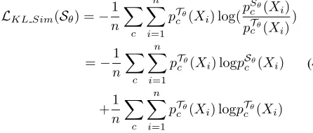
KL-divergenceis a measure of how one probability distri-bution is different from another reference probability dis-tribution. Here we train student networkSθby minimizing

the KL-divergence between its outputpSθ

c (Xi)and the soft

labelspTθ

c (Xi)generated by the teacher network. Our loss

function is:

LKL Sim(Sθ) =−

1 n

X

c n

X

i=1 pTθ

c (Xi) log(

pSθ

c (Xi)

pTθ

c (Xi)

)

=−1

n

X

c n

X

i=1 pTθ

c (Xi) logpScθ(Xi)

+1 n

X

c n

X

i=1 pTθ

c (Xi) logpTcθ(Xi)

(4)

where the second term is the entropy of soft labels from teacher network and is constant with respect toTθ. We can

remove it and simply minimize the cross-entropy loss as fol-lows:

LCE Sim(Sθ) =−

1 n

X

c n

X

i=1 pTθ

c (Xi) logpScθ(Xi) (5)

4.2 Intermediate Alignment

Adaptive Pooling. The purpose of the adaptive pooling layer is to align the intermediate output from teacher net-work and student netnet-work. This kind of layer is similar to the ordinary pooling layer like average or max pooling, but can generate a predefined length of output with different in-put size. Because of this specialty, we can use the different teacher networks and pool the output to the same length of student output. Pooling layer can also achieve spatial invari-ance when reducing the resolution of feature maps. Thus, for the intermediate output, our loss function is:

Lj_Sim=d(f(Tθj), f(Sθj)) (6)

where Tθj and Sθj are the outputs at j-th layer of the

teacher and student, respectively.f is the adaptive pooling function that can be average or max. Fig. 5 illustrates the process of adaptive pooling. Because we adopt multiple in-termediate layers, our final similarity loss is a sum of indi-vidual one:

0.9 0.1 0.6 0.2 0.3

adaptive pooling 0.5

0 0 2

0.7

indices

0.9 0.6 0.7 values Forward

0.3 0 0.5 0 0 0

0 0 2

0.1

indices

0.3 0.5 0.1 gradients backward

output size = 3

Figure 5: The process of adaptive pooling in forward and backward stages. We use max operation for illustration.

LSim=

X

j∈A

Lj_Sim (7)

whereAis the set of layers that we choose to produce out-put. In our experiments, we use the last layer in each block of a network (block-wise).

4.3 Stacked Discriminators

We generate student output by training the student network

Sθ and freezing the teacher parts adversarially against a

series of stacked discriminators Dj. A discriminatorD

at-tempts to classify its inputxas teacher or student by maxi-mizing the following objective (Goodfellow et al. 2014):

Lj_GAN = _E

x∼pteacher

logDj(x) + E

x∼pstudent

log(1−Dj(x)) (8)

where x∼pstudent are outputs from generation network Sθj. At the same time,Sθj attempts to generate similar

out-puts which will fool the discriminator by minimizingLj_GAN. Since the parameters of our teacher are fixed during train-ing, the first term can be removed and our final objective loss is:

Lj_GAN = _E

x∼pstudent

log(1−Dj(x)) (9)

In Eq. 10,xis the concatenation of teacher and student outputs. We feedxinto the discriminator which is a three-layer fully-connected network. The whole structure of a dis-criminator is shown in Fig. 4.

Multi-Stage Discriminators. Using multi-Stage discrimi-nators can refine the student outputs gradually. As shown in Fig. 3, the final adversarial loss is a sum of the individual ones:

LGAN=

X

j∈A

Lj_GAN (10)

Let|A|be the number of discriminators. In our experiments, we use 3 for CIFAR (Krizhevsky 2009) and SVHN (Netzer et al. 2011), and 5 for ImageNet (Deng et al. 2009).

4.4 Joint Training of Similarity and Discriminators

Based on above definition and analysis, we incorporate the similarity loss in Eq. 7 and adversarial loss in Eq. 10 into our final loss function. Our whole framework is trained end-to-end by the following objective function:

L=αLSim+βLGAN (11)

5. Multi-Model Ensemble via Adversarial

Learning (MEAL)

We achieve ensemble with a training method that is sim-ple and straight-forward to imsim-plement. As different net-work structures can obtain different distributions of outputs, which can be viewed as soft labels (knowledge), we adopt these soft labels to train our student, in order to compress knowledge of different architectures into a single network. Thus we can obtain the seemingly contradictory goal of en-sembling multiple neural networks atno additional testing

cost.

5.1 Learning Procedure

To clearly understand what the student learned in our work, we define two conditions. First, the student has the same structure as the teacher network. Second, we choose one structure for student and randomly select a structure for teacher in each iteration as our ensemble learning procedure. The learning procedure contains two stages. First, we pre-train the teachers to produce a model zoo. Because we use the classification task to train these models, we can use the softmax cross entropy loss as the main training loss in this stage. Second, we minimize the loss functionLin Eq. 11 to make the student output similar to that of the teacher output. The learning procedure is explained below in Algorithm 1.

Algorithm 1Multi-Model Ensemble via Adversarial Learn-ing (MEAL).

Stage 1:

Building and Pre-training the Teacher Model Zoo T =

{T1

θ,Tθ2, . . .Tθi}, including: VGGNet (Simonyan and Zisserman

2015), ResNet (He et al. 2016), DenseNet (Huang et al. 2017b), MobileNet (Howard et al. 2017), Shake-Shake (Gastaldi 2017), etc. Stage 2:

1: functionT SM(T)

2: Tθ←RS(T) .Random Selection

3: returnTθ

4: end function 5: foreach iterationdo:

6: Tθ←T SM(T) .Randomly Select a Teacher Model

7: Sθ= arg minS_θ L(Tθ,Sθ) .Adversarial Learning for a

Student 8: end for

6. Experiments and Analysis

We empirically demonstrate the effectiveness of MEAL on several benchmark datasets. We implement our method on the PyTorch (Paszke et al. 2017) platform.

6.1. Datasets

CIFAR.The two CIFAR datasets (Krizhevsky 2009) con-sist of colored natural images with a size of 32×32. CIFAR-10 is drawn from CIFAR-10 and CIFAR-CIFAR-100 is drawn from CIFAR-100 classes. In each dataset, the train and test sets contain 50,000 and 10,000 images, respectively. A standard data

augmenta-tion scheme3 (Lee et al. 2015; Romero et al. 2015; Lars-son, Maire, and Shakhnarovich 2016; Huang et al. 2017a; Liu et al. 2017) is used. We report the test errors in this sec-tion with training on the whole training set.

SVHN. The Street View House Number (SVHN) dataset (Netzer et al. 2011) consists of 32×32 colored digit images, with one class for each digit. The train and test sets contain 604,388 and 26,032 images, respec-tively. Following previous works (Goodfellow et al. 2013; Huang et al. 2016; 2017a; Liu et al. 2017), we split a subset of 6,000 images for validation, and train on the remaining images without data augmentation.

ImageNet.The ILSVRC 2012 classification dataset (Deng et al. 2009) consists of 1000 classes, with a number of 1.2 million training images and 50,000 validation im-ages. We adopt the the data augmentation scheme follow-ing (Krizhevsky, Sutskever, and Hinton 2012) and apply the same operation as (Huang et al. 2017a) at test time.

6.2 Networks

We adopt several popular network architectures as our teacher model zoo, including VGGNet (Simonyan and Zis-serman 2015), ResNet (He et al. 2016), DenseNet (Huang et al. 2017b), MobileNet (Howard et al. 2017), shake-shake (Gastaldi 2017), etc. For VGGNet, we use 19-layer with Batch Normalization (Ioffe and Szegedy 2015). For ResNet, we use 18-layer network for CIFAR and SVHN and 50-layer for ImagNet. For DenseNet, we use theBC struc-ture with depth L=100, and growth rate k=24. For shake-shake, we use 26-layer 2×96d version. Note that due to the high computing costs, we use shake-shake as a teacher only when the student is shake-shake network.

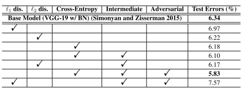
Table 1: Ablation study on CIFAR-10 using VGGNet-19 w/BN. Please refer to Section 6.3 for more details.

`1dis. `2dis. Cross-Entropy Intermediate Adversarial Test Errors (%)

Base Model (VGG-19 w/ BN) (Simonyan and Zisserman 2015) 6.34

! 6.97

! 6.22

! 6.18

! ! 6.10

! ! 6.17

! ! ! 5.83

! ! ! 7.57

6.3 Ablation Studies

We first investigate each design principle of our MEAL framework. We design several controlled experiments on CIFAR-10 with VGGNet-19 w/BN (both to teacher and stu-dent) for this ablation study. A consistent setting is imposed on all the experiments, unless when some components or structures are examined.

The results are mainly summarized in Table 1. The first three rows indicate that we only use`1,`2or cross-entropy

3

CIFAR-10 3.50

3.55 3.60 3.65 3.70 3.75 3.80

Test Error (%)

3.76

3.74 _3.73

3.56

Single Single AL True Ens. Our Ens.

CIFAR-100 17

18 19 20

Test Error (%)

20.23

19.04

17.73 17.21

Single Single AL True Ens. Our Ens.

SVHN 1.60

1.65 1.70 1.75 1.80

Test Error (%)

1.77

1.69 1.66

1.64

Single Single AL True Ens. Our Ens.

ImageNet 21.0

21.5 22.0 22.5 23.0 23.5 24.0

Top-1 Test Error (%)

23.85 _23.71

22.76

21.69

Single Single AL True Ens. Our Ens.

Figure 6: Error rates (%) on CIFAR-10 and CIFAR-100, SVHN and ImageNet datasets. In each figure, the results from left to right are 1) base model; 2) base model with adversarial learning; 3) true ensemble/traditional ensemble; and 4) our ensemble results. For the first three datasets, we employ DenseNet as student, and ResNet for the last one (ImageNet).

loss from the last layer of a network. It’s similar to the

Knowledge Distillation method. We can observe that use

cross-entropy achieve the best accuracy. Then we employ more intermediate outputs to calculate the loss, as shown in rows 4 and 5. It’s obvious that including more layers im-proves the performance. Finally, we involve the discrimina-tors to exam the effectiveness of adversarial learning. Using cross-entropy, intermediate layers and adversarial learning achieve the best result. Additionally, we use average based adaptive pooling for alignment. We also tried max operation, the accuracy is much worse (6.32%).

6.4 Results

Comparison with Traditional Ensemble. The results are summarized in Figure 6 and Table 2. In Figure 6, we com-pare the error rate using the same architecture on a vari-ety of datasets (except ImageNet). It can be observed that our results consistently outperform the single and traditional methods on these datasets. The traditional ensembles are obtained through averaging the final predictions across all teacher models. In Table 2, we compare error rate using dif-ferent architectures on the same dataset. In most cases, our ensemble method achieves lower error than any of the base-lines, including the single model and traditional ensemble.

Table 2: Error rate (%) using different network architectures on CIFAR-10 dataset.

Network Single (%) Traditional Ens. (%) Our Ens. (%)

MobileNet (Howard et al. 2017) 10.70 – 8.09

VGG-19 w/ BN (Simonyan and Zisserman 2015) 6.34 – 5.55

DenseNet-BC (k=24) (Huang et al. 2017b) 3.76 3.73 3.54

Shake-Shake-26 2x96d (Gastaldi 2017) 2.86 2.79 2.54

Comparison with Dropout.We compare MEAL with the “Implicit” method Dropout (Srivastava et al. 2014). The re-sults are shown in Table 3, we employ several network ar-chitectures in this comparison. All models are trained with the same epochs. We use a probability of 0.2 for drop nodes during training. It can be observed that our method achieves better performance than Dropout on all these networks.

Our Learning-Based Ensemble Results on ImageNet.As shown in Table 4, we compare our ensemble method with the original model and the traditional ensemble. We use VGG-19 w/BN and 50 as our teachers, and use ResNet-50 as the student. The #FLOPs and inference time for

tra-Table 3: Comparison of error rate (%) with Dropout (Srivas-tava et al. 2014) baseline on CIFAR-10.

Network Dropout (%) Our Ens. (%)

VGG-19 w/ BN (Simonyan and Zisserman 2015) 6.89 5.55

GoogLeNet (Szegedy et al. 2015) 5.37 4.83

ResNet-18 (He et al. 2016) 4.69 4.35

DenseNet-BC (k=24) (Huang et al. 2017b) 3.75 3.54

ditional ensemble are the sum of individual ones. There-fore, our method has both better performance and higher efficiency. Most notably, our MEAL Plus4 _{yields an error}

rate of Top-1 21.79%, Top-5 5.99% on ImageNet, far out-performing the original ResNet-50 23.85%/7.13% and the traditional ensemble 22.76%/6.49%. This shows great po-tential on large-scale real-size datasets.

Table 4: Val. error (%) on ImageNet dataset.

Method Top-1 (%) Top-5 (%) #FLOPs Inference Time (per/image) Teacher Networks:

VGG-19 w/BN 25.76 8.15 19.52B 5.70×10−3_s

ResNet-50 23.85 7.13 4.09B 1.10×10−2_s

Ours (ResNet-50) 23.58 6.86 4.09B 1.10×10−2_s

Traditional Ens. 22.76 6.49 23.61B 1.67×10−2_s

Ours Plus (ResNet-50) 21.79 5.99 4.09B 1.10×10−2_s

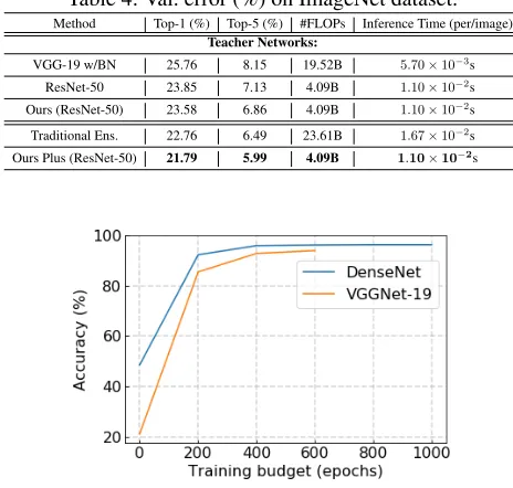
Figure 7: Accuracy of our ensemble method under different training budgets on CIFAR-10.

4

1 2 3 4 5 # of ensembles 7.5

8.0 8.5 9.0 9.5 10.0

Test Error (%)

MobileNet

MobileNet baseline: 10.70% (Howard et al. 2017)

1 2 3 4 5

# of ensembles 5.5

5.6 5.7 5.8 5.9 6.2 6.7

Test Error (%)

VGG19-BN

VGG19-BN baseline: 6.34% (Simonyan et al. 2015)

1 2 3 4 5

# of ensembles 3.50

3.55 3.60 3.65 3.70 3.75

Test Error (%)

DenseNet

DenseNet baseline: 3.76% (Huang et al. 2017)

Figure 8: Error rate (%) on CIFAR-10 with MobileNet, VGG-19 w/BN and DenseNet.

Figure 9: Probability Distributions between four net-works. Left: SequeezeNet vs. VGGNet. Right: ResNet vs.

DenseNet.

6.5 Analysis

Effectiveness of Ensemble Size.Figure 8 displays the per-formance of three architectures on CIFAR-10 as the ensem-ble size is varied. Although ensembling more models gener-ally gives better accuracy, we have two important observa-tions. First, we observe that our single model “ensemble” al-ready outputs the baseline model with a remarkable margin, which demonstrates the effectiveness of adversarial learn-ing. Second, we observe some drops in accuracy using the VGGNet and DenseNet networks when including too many ensembles for training. In most case, an ensemble of four models obtains the best performance.

Budget for Training. On CIFAR datasets, the standard training budget is 300 epochs. Intuitively, our ensemble method can benefit from more training budget, since we use the diverse soft distributions as labels. Figure 7 displays the relation between performance and training budget. It ap-pears that more than 400 epochs is the optimal choice and our model will fully converge at about 500 epochs.

Diversity of Supervision.We hypothesize that different ar-chitectures create soft labels which are not only informative but also diverse with respect to object categories. We qualita-tively measure this diversity by visualizing the pairwise cor-relation of softmax outputs from two different networks. To do so, we compute the softmax predictions for each training image in ImageNet dataset and visualize each pair of the cor-responding ones. Figure 9 displays the bubble maps of four architectures. In the left figure, the coordinate of each bubble is a pair ofk-th predictions (pk_{SequeezeN et}, pk_{V GGN et}),k =

Figure 10: Visualizations of validation images from the Ima-geNet dataset by t-SNE (Maaten and Hinton 2008). We ran-domly sample 10 classes within 1000 classes. Left is the sin-gle model result using the standard training strategy. Right is our ensemble model result.

1,2, . . . ,1000, and the right figure is (pk_{ResN et}, pk_{DenseN et}). If the label distributions are identical from two networks, the bubbles will be placed on the master diagonal. It’s very in-teresting to observe that the left (weaker network pairs) has bigger diversity than the right (stronger network pairs). It makes sense because the stronger models generally tend to generate predictions close to the ground-truth. In brief, these differences in predictions can be exploited to create effective ensembles and our method is capable of improving the com-petitive baselines using this kind of diverse supervisions.

6.6 Visualization of the Learned Features

To further explore what our model actually learned, we vi-sualize the embedded features from the single model and our ensembling model. The visualization is plotted by t-SNE tool (Maaten and Hinton 2008) with the last conv-layer features (2048 dimensions) from ResNet-50. We randomly sample 10 classes on ImageNet, results are shown in Fig-ure 10, it’s obvious that our model has better featFig-ure embed-ding result.

7. Conclusion

AcknowledgementsThis work was supported in part by Na-tional Key R&D Program of China (No.2017YFC0803700), NSFC under Grant (No.61572138 & No.U1611461) and STCSM Project under Grant No.16JC1420400.

References

Anil, R.; Pereyra, G.; Passos, A.; Ormandi, R.; Dahl, G. E.; and Hinton, G. E. 2018. Large scale distributed neural network training through online distillation. InICLR.

Bagherinezhad, H.; Horton, M.; Rastegari, M.; and Farhadi, A. 2018. Label refinery: Improving imagenet classification through label progression. InECCV.

Bai, Y.; Zhang, Y.; Ding, M.; and Ghanem, B. 2018. Finding tiny faces in the wild with generative adversarial network.

Chen, T.; Goodfellow, I.; and Shlens, J. 2016. Net2net: Accelerat-ing learnAccelerat-ing via knowledge transfer. InICLR.

Deng, J.; Dong, W.; Socher, R.; Li, L.-J.; et al. 2009. Imagenet: A large-scale hierarchical image database. InCVPR.

Dietterich, T. G. 2000. Ensemble methods in machine learning. In International workshop on multiple classifier systems, 1–15.

Gastaldi, X. 2017. Shake-shake regularization. arXiv preprint

arXiv:1705.07485.

Goodfellow, I. J.; Warde-Farley, D.; Mirza, M.; Courville, A.; and

Bengio, Y. 2013. Maxout networks. InICML.

Goodfellow, I.; Pouget-Abadie, J.; Mirza, M.; Xu, B.; Warde-Farley, D.; Ozair, S.; Courville, A.; and Bengio, Y. 2014. Gen-erative adversarial nets. InNIPS.

Hansen, L. K., and Salamon, P. 1990. Neural network

ensem-bles. IEEE transactions on pattern analysis and machine

intelli-gence12(10):993–1001.

He, K.; Zhang, X.; Ren, S.; and Sun, J. 2016. Deep residual learn-ing for image recognition. InCVPR.

Hinton, G.; Vinyals, O.; and Dean, J. 2015. Distilling the knowl-edge in a neural network.arXiv preprint arXiv:1503.02531. Howard, A. G.; Zhu, M.; Chen, B.; Kalenichenko, D.; Wang, W.; Weyand, T.; Andreetto, M.; and Adam, H. 2017. Mobilenets: Effi-cient convolutional neural networks for mobile vision applications. arXiv preprint arXiv:1704.04861.

Huang, G.; Sun, Y.; Liu, Z.; Sedra, D.; and Weinberger, K. Q. 2016.

Deep networks with stochastic depth. InECCV.

Huang, G.; Li, Y.; Pleiss, G.; Liu, Z.; Hopcroft, J. E.; and Wein-berger, K. Q. 2017a. Snapshot ensembles: Train 1, get m for free. InICLR.

Huang, G.; Liu, Z.; Weinberger, K. Q.; and van der Maaten, L.

2017b. Densely connected convolutional networks. InCVPR.

Ioffe, S., and Szegedy, C. 2015. Batch normalization: Accelerating deep network training by reducing internal covariate shift. arXiv preprint arXiv:1502.03167.

Johnson, J.; Gupta, A.; and Fei-Fei, L. 2018. Image generation

from scene graphs. InCVPR.

Krizhevsky, A.; Sutskever, I.; and Hinton, G. 2012. Imagenet clas-sification with deep convolutional neural networks. InNIPS. Krizhevsky, A. 2009. Learning multiple layers of features from tiny images. Technical report.

Krogh, A., and Vedelsby, J. 1995. Neural network ensembles, cross validation, and active learning. InNIPS.

Lakshminarayanan, B.; Pritzel, A.; and Blundell, C. 2017. Simple and scalable predictive uncertainty estimation using deep ensem-bles. InNIPS.

Larsson, G.; Maire, M.; and Shakhnarovich, G. 2016. Fractal-net: Ultra-deep neural networks without residuals. arXiv preprint

arXiv:1605.07648.

Lee, C.-Y.; Xie, S.; Gallagher, P. W.; et al. 2015. Deeply-supervised nets. InAISTATS.

Li, Y.; Yang, J.; Song, Y.; Cao, L.; Luo, J.; and Li, L.-J. 2017. Learning from noisy labels with distillation. InICCV.

Liu, Z.; Li, J.; Shen, Z.; Huang, G.; Yan, S.; and Zhang, C. 2017. Learning efficient convolutional networks through network slim-ming. InICCV.

Maaten, L. v. d., and Hinton, G. 2008. Visualizing data using t-sne.

Journal of machine learning research9(Nov):2579–2605.

Netzer, Y.; Wang, T.; Coates, A.; Bissacco, A.; Wu, B.; and Ng, A. Y. 2011. Reading digits in natural images with unsupervised

feature learning. InNIPS workshop on deep learning and

unsuper-vised feature learning, volume 2011, 5.

Papernot, N.; Abadi, M.; Erlingsson, U.; Goodfellow, I.; and Tal-war, K. 2017. Semi-supervised knowledge transfer for deep learn-ing from private trainlearn-ing data. InICLR.

Paszke, A.; Gross, S.; Chintala, S.; Chanan, G.; Yang, E.; DeVito, Z.; Lin, Z.; Desmaison, A.; Antiga, L.; and Lerer, A. 2017. Auto-matic differentiation in pytorch.

Perrone, M. P., and Cooper, L. N. 1995. When networks disagree:

Ensemble methods for hybrid neural networks. InHow We Learn;

How We Remember: Toward an Understanding of Brain and Neu-ral Systems: Selected Papers of Leon N Cooper. World Scientific. 342–358.

Romero, A.; Ballas, N.; Kahou, S. E.; Chassang, A.; Gatta, C.; and Bengio, Y. 2015. Fitnets: Hints for thin deep nets. InICLR. Simonyan, K., and Zisserman, A. 2015. Very deep convolutional networks for large-scale image recognition. InICLR.

Singh, S.; Hoiem, D.; and Forsyth, D. 2016. Swapout: Learning an ensemble of deep architectures. InAdvances in neural information processing systems, 28–36.

Srivastava, N.; Hinton, G. E.; Krizhevsky, A.; et al. 2014. Dropout: a simple way to prevent neural networks from overfitting.JMLR. Szegedy, C.; Liu, W.; Jia, Y.; Sermanet, P.; et al. 2015. Going

deeper with convolutions. InCVPR.