Rank Determination for Low-Rank Data Completion

Rank Determination for Low-Rank Data Completion

Morteza Ashraphijuo [email protected]

Columbia University New York, NY 10027, USA

Xiaodong Wang [email protected]

Columbia University New York, NY 10027, USA

Vaneet Aggarwal [email protected]

Purdue University

West Lafayette, IN 47907, USA

Editor:Animashree Anandkumar

Abstract

Recently, fundamental conditions on the sampling patterns have been obtained for finite com-pletability of low-rank matrices or tensors given the corresponding ranks. In this paper, we consider the scenario where the rank is not given and we aim to approximate the unknown rank based on the location of sampled entries and some given completion. We consider a number of data models, including single-view matrix, multi-view matrix, CP tensor, tensor-train tensor and Tucker tensor. For each of these data models, we provide an upper bound on the rank when an arbitrary low-rank completion is given. We characterize these bounds both deterministically, i.e., with probability one given that the sampling pattern satisfies certain combinatorial properties, and probabilistically, i.e., with high probability given that the sampling probability is above some threshold. Moreover, for both single-view matrix and CP tensor, we are able to show that the obtained upper bound is ex-actly equal to the unknown rank if the lowest-rank completion is given. Furthermore, we provide numerical experiments for the case of single-view matrix, where we use nuclear norm minimiza-tion to find a low-rank compleminimiza-tion of the sampled data and we observe that in most of the cases the proposed upper bound on the rank is equal to the true rank.

Keywords: Low-rank data completion, rank estimation, tensor, matrix, manifold, Tucker rank, tensor-train rank, CP rank, multi-view matrix.

1. Introduction

Developing methods and algorithms to study large high-dimensional data is becoming more indis-pensable as hyperspectral images and videos, product ranking datasets and other applications of big datasets are attracting more attention recently. Moreover, in order to guarantee the same level of efficiency in images or videos, a minor increment in dimensionality in the datasets entails a sig-nificant increment in the amount of the data, and this fact causes modeling and also computational challenges to analyze big high-dimensional datasets. Consequently, providing a statistically rig-orous result requires a massive amount of data that grows exponentially with the dimension. The low-rank data completion problem is concerned with completing a matrix or tensor given a subset of its entries and some rank constraints. Various applications can be found in many fields includ-ing image and signal processinclud-ing (Cand`es et al., 2013; Ji et al., 2010), data mininclud-ing (Eld´en, 2007),

c

network coding (Harvey et al., 2005), compressed sensing (Lim and Comon, 2010; Sidiropoulos and Kyrillidis, 2012; Ashraphijuo et al., 2016c; Gandy et al., 2011; Ashraphijuo and Wang, 2017c; Ashraphijuo et al., 2015), reconstructing the visual data (Liu et al., 2013), bioinformatics and sys-tems biology (Ogundijo et al., 2017; Ogundijo et al.), fingerprinting (Liu et al., 2016), etc. There is an extensive literature on developing various optimization methods to treat this problem including minimizing a convex relaxation of rank (Cand`es and Recht, 2009; Cand`es and Tao, 2010; Cai et al., 2010; Gandy et al., 2011; Ashraphijuo et al., 2016b; Ashraphijuo and Wang, 2017c), non-convex approaches (Recht and R´e, 2013), and alternating minimization (Jain et al., 2013; Ge et al., 2016), etc. More recently, deterministic conditions on the sampling patterns have been studied for sub-space clustering in (Pimentel-Alarc´on et al., 2016c, 2015, 2016a,b). Moreover, the fundamental conditions on the sampling pattern that lead to different numbers of completion (unique, finite, or infinite) for different data structures given the corresponding rank constraints have been investi-gated in (Pimentel-Alarc´on et al., 2016d; Ashraphijuo et al., 2017c; Ashraphijuo and Wang, 2017b; Ashraphijuo et al., 2016a; Ashraphijuo and Wang, 2017a; Ashraphijuo et al., 2017d,a,b).

However, in many practical low-rank data completion problems, the rank may not be known

a priori. In this paper, we investigate this problem and we aim to approximate the rank based on the given entries, where it is assumed that the original data is generically chosen from the manifold corresponding to the unknown rank. The only existing work that treats this problem for a single-view matrix data based on the sampling pattern is (Pimentel-Alarc´on and Nowak, 2016), which requires some strong assumptions including the existence of a completion whose rankr is a lower bound on the unknown true rankr∗, i.e.,r∗ ≥r. We start by investigating the single-view matrix to provide a new analysis that does not require such assumption and also we can extend our approach to treat the CP rank tensor model. Moreover, we further generalize our approach to treat vector rank data models including the multi-view matrix, the Tucker rank tensor and the tensor-train (TT) rank tensor. For each of these data models, we obtain the upper bound on the scalar rank or component-wise upper bound on the unknown vector rank, deterministically based on the sampling pattern and the rank of a given completion. We also obtain such bound that holds with high probability based on the sampling probability. Moreover, for the single-view matrix, we provide some numerical results to show how tight our probabilistic bounds on the rank are (in terms of the sampling probability). In particular, we used nuclear norm minimization to find a completion and demonstrate our proposed method in obtaining a tight bound on the unknown rank.

In general, providing a completion requires much less samples than recovering the original sampled data. The goal of this paper is to solve the fundamental problem of rank determination for the original sampled data given an arbitrary low-rank data completion. One possible application scenario is to improve upon the low-rank completion obtained by the convex relaxation methods. Specifically, using convex optimization (minimization of nuclear and atomic norms or summation of nuclear norms of matricizations and unfoldings) or any other methods in the literature, we may be able to find a fairly low-rank “completion” of the original data, which is not necessarily equal (or even close) to the original sampled data. Then, under some circumstances, the rank of the obtained completion using any rank independent method can be an upper bound on the rank of the original sampled data (and sometimes the obtained rank can be exactly equal to the rank of the original sampled data).

Ashraphi-juo et al., 2016a; AshraphiAshraphi-juo and Wang, 2017a) such that given an arbitrary low-rank completion we can provide a tight upper bound on the rank. To illustrate how such approximation is even pos-sible consider the following example. Assume that ann1×n2rank-2matrix is chosen generically

from the corresponding manifold. Hence, any2×2submatrix of this matrix is full-rank with proba-bility one (due to the genericity assumption). Moreover, note that any3×3submatrix of this matrix is not full-rank. As a result, by observing the sampled entries we can find some bounds on the rank. Using the analysis in (Pimentel-Alarc´on et al., 2016d; Ashraphijuo et al., 2017c; Ashraphijuo and Wang, 2017b; Ashraphijuo et al., 2016a; Ashraphijuo and Wang, 2017a) on finite completablity of the sampled data (finite number of completions) for different data models, we characterize both deterministic and probablistic bounds on the unknown rank.

The remained of the paper is organized as follows. In Section 2, we introduce the data models and problem statement. In Sections 3 and 4 we characterize our determintic and probablistic bounds for scalar-rank cases (single-view matrix and CP tensor) and vector-rank cases (multi-view matrix, Tucker tensor and TT tensor), respectively. Finally, Section 5 concludes the paper.

2. Data Models and Problem Statement

2.1 Matrix Models

2.1.1 SINGLE-VIEWMATRIX

Assume that the sampled matrixUis chosen generically from the manifold of then1×n2matrices

of rankr∗, wherer∗ is unknown. The matrixV ∈ Rn1×r

∗

is called a basis forUif each column ofUcan be written as a linear combination of the columns ofV. DenoteΩas the binary sampling pattern matrix that is of the same size asU and Ω(~x) = 1 if U(~x) is observed andΩ(~x) = 0

otherwise, where~x = (x1, x2)represents the entry corresponding to row number x1 and column

numberx2. Moreover, defineUΩas the matrix obtained from samplingUaccording toΩ, i.e.,

UΩ(~x) =

U(~x) if Ω(~x) = 1,

0 if Ω(~x) = 0. (1)

2.1.2 MULTI-VIEWMATRIX

The matrixU ∈ _Rn×(n1+n2) _{is sampled. Denote a partition ofUasU = [U}

1|U2]whereU1 ∈ Rn×n1 andU2 ∈ Rn×n2 represent the first and second views of data, respectively. The sampling pattern is defined asΩ= [Ω1|Ω2], whereΩ1andΩ2represent the sampling patterns corresponding

to the first and second views of data, respectively. Assume that rank(U1) =r∗1, rank(U2) =r∗2and

rank(U) =r∗, and alsoUis chosen generically from the manifold structure with above parameters. Denoter∗ = (r∗₁, r₂∗, r∗)which is assumed unknown.

2.2 Tensor Models

Assume that ad-way tensorU ∈_Rn1×···×nd_{is sampled. For the sake of simplicity in notation, define} Ni ,

Πi_j=1nj

, N¯i ,

Πd_j=i+1nj

andN−i , N_nd_i. DenoteΩas the binary sampling pattern

as the tensor obtained from samplingU according toΩ, i.e.,

UΩ(~x) =

U(~x) if Ω(~x) = 1,

0 if Ω(~x) = 0. (2)

For each subtensor U0 _{of the tensor U, define N}

Ω(U0) as the number of observed entries in U0

according to the sampling patternΩ. Define the matrixUe_(i)∈_RNi×

¯

Ni _{as thei-thunfoldingof the tensorU, such thatU(~x) =} e

U(i)(Mfi(x1, . . . , xi),M−f i(xi+1, . . . , xd)), whereMfi : (x1, . . . , xi) → {1,2, . . . , Ni}andM−f i :

(xi+1, . . . , xd)→ {1,2, . . . ,N¯i}are two bijective mappings.

LetU(i) ∈Rni×N−ibe thei-thmatricizationof the tensorU, such thatU(~x) =U(i)(xi, Mi(x1,

. . . , xi−1, xi+1, . . . , xd)), where Mi : (x1, . . . , xi−1, xi+1, . . . , xd) → {1,2, . . . , N−i}is a

bijec-tive mapping. Observe that for any arbitrary tensorA, the first matricization and the first unfolding are the same, i.e.,A(1) =Ae₍₁₎.

In what follows, we introduce three different tensor ranks, i.e., the CP rank, Tucker rank and TT rank.

2.2.1 CP DECOMPOSITION

The CP rank of a tensorU, rankCP(U) = r, is defined as the minimum numberr such that there existal_i ∈_Rni_{for1≤i≤dand1≤l≤r, such that}

U =

r

X

l=1

al₁⊗al₂⊗. . .⊗al_d, (3)

or equivalently,

U(x1, x2, . . . , xd) = r

X

l=1

al₁(x1)al2(x2). . .ald(xd), (4)

where⊗denotes the tensor product (outer product) andal_i(xi)denotes thexi-th entry of vectorali.

Note thatal₁⊗al₂⊗. . .⊗al_d∈_Rn1×···×nd _{is a rank-1tensor,l= 1,2, . . . , r.}

2.2.2 TUCKERDECOMPOSITION

GivenU ∈Rn1×···×nd _andX∈Rni×n0i, the productU0 ,U ×_iX ∈_Rn1×···×ni−1×n0_i×ni+1×···×nd is defined as

U0(x1,· · ·, xi−1, ki, xi+1,· · ·, xd), ni X

xi=1

U(x1,· · ·, xi−1, xi, xi+1,· · ·, xd)X(xi, ki). (5)

The Tucker rank of a tensor U is defined as rankTucker(U) = r = (m1, . . . , md) where mi =

rank(U_(i)), i.e., the rank of thei-th matricization,i= 1, . . . , d. The Tucker decomposition ofU is given by

U(~x) =

m1

X

k1=1 · · ·

md X

kd=1

or in short

U =C ×d_i=1Ti, (7)

whereC ∈Rm1×···×md _{is the core tensor andT}

i ∈Rmi×niaredorthogonal matrices. 2.2.3 TT DECOMPOSITION

The separation or TT rank of a tensor is defined as rankTT(U) = r = (u1, . . . , ud−1)whereui =

rank(Ue_(i)), i.e., the rank of thei-th unfolding,i = 1, . . . , d−1. Note thatu_i ≤ max{N_i,N¯_i}in general and alsou1is simply the conventional matrix rank whend= 2. The TT decomposition of

a tensorU is given by

U(~x) =

u1

X

k1=1 · · ·

ud−1

X

kd−1=1 U(1)_(x

1, k1) d−1

Y

i=2

U(i)_(k

i−1, xi, ki)

!

U(d)_(k

d−1, xd), (8)

or in short

U =U(1). . .U(d), (9)

where the3-way tensorsU(i)_∈

Rui−1×ni×ui fori= 2, . . . , d−1and matricesU(1) ∈Rn1×u1 and

U(d) _∈

Rud−1×nd are the components of this decomposition.

For each matrix or tensor model, we assume that the true rank ofU orU isr∗ orr∗ which is unknown, and alsoUorU is chosen generically from the corresponding manifold. The table below represents the mentioned symbols in brief.

Data structure Sampled data Rank Comments Single-view matrix U∈_Rn1×n2 _r∗ _–

Multi-view matrix U= [U1|U2]∈Rn×(n1+n2) r∗ = (r1∗, r2∗, r∗) r∗i =rank(Ui)

CP tensor U ∈_Rn1×···×nd _r∗ _– Tucker tensor U ∈Rn1×···×nd _r∗ _{= (m}∗

1, . . . , m∗d) m

∗

i =rank(U(i))

TT tensor U ∈_Rn1×···×nd _r∗ _{= (u}∗

1, . . . , u∗d−1) u

∗

i =rank(Ue_(i))

2.3 Problem Statement

3. Scalar-Rank Cases

3.1 Single-View Matrix

Previously, this problem has been treated in (Pimentel-Alarc´on and Nowak, 2016), where strong assumptions including the existence of a completion with rank r ≤ r∗ have been used. In this section, we provide an analysis that does not require such assumption and moreover our analysis can be extended to multi-view data and tensors in the following sections. Furthermore, we show the tightness of our theoretical bounds via numerical examples.

Assume thatU∈_Rn1×n2 _{is the sampled matrix. Let}

P1 andP2denote the Lebesgue measures

onRn1×r

∗

andRr

∗_×n

2_{, respectively. In this paper, we assume that the matrixUis chosen}

generi-cally from the manifold ofn1×n2matrices of rankr∗, i.e., the entries ofUare drawn independently

with respect to Lebesgue measure on the corresponding manifold. Hence, the probability measures of all statements in this subsection areP1×P2.

3.1.1 DETERMINISTICRANKANALYSIS

The following condition will be used frequently in this subsection.

ConditionAr: Each column of the sampled matrix includes at leastrsampled entries.

Consider an arbitrary column of the sampled matrixU(:, i), wherei∈ {1, . . . , n2}. Letli =

NΩ(U(:, i))denote the number of observed entries in thei-th column ofU. ConditionArresults

thatli≥r.

We construct a binary valued matrix called constraint matrix Ω˘r based on Ω and a given

numberr. Specifically, we constructli−rcolumns with binary entries based on the locations of the

observed entries inU(:, i)such that each column has exactlyr+1entries equal to one. Assume that x1, . . . , xli are the row indices of all observed entries in this column. LetΩ

i

rbe the corresponding

n1×(li−r)matrix to this column which is defined as the following: for anyj ∈ {1, . . . , li−r},

thej-th column has the value1in rows{x1, . . . , xr, xr+j}and zeros elsewhere. Define the binary

constraint matrix as Ω˘r =

Ω1_r|Ω2_r. . .|Ωn2

r

∈ _Rn1×Kr _{(Pimentel-Alarc´on et al., 2016d), where} Kr=NΩ(U)−n2r.

ConditionBr: There exists a submatrix1Ω˘0r ∈Rn1×K ofΩ˘rsuch thatK =n1r−r2and for

anyK0∈ {1,2, . . . , K}and any submatrixΩ˘_r00∈_Rn1×K0 _ofΩ˘0

rwe have

rf(Ω˘00_r)−r2 ≥K0, (10) wheref(Ω˘00_r)denotes the number of nonzero rows ofΩ˘00_r.

Note that exhaustive enumeration is needed in order to check whether or not Condition Br

holds. Hence, the deterministic analysis cannot be used in practice for large-scale data. However, it serves as the basis of the subsequent probabilistic analysis that will lead to a simple lower bound on the sampling probability such that ConditionBr holds with high probability, which is of practical

value.

In the following, we restate Theorem1in (Pimentel-Alarc´on et al., 2016d) which will be used later.

Lemma 1 With probability one, there are finitely many completions of the sampled matrix if and only if ConditionsAr∗andB_r∗ hold.

Recall that the true rankr∗is assumed unknown.

Definition 2 LetS_Ωdenote the set of all natural numbersrsuch that both ConditionsAr andBr hold.

Lemma 3 There exists a numberrΩsuch thatSΩ={1,2, . . . , rΩ}.

Proof Assume that 1 < r ≤ min{n1, n2} and r ∈ SΩ. It suffices to showr −1 ∈ SΩ. By

contradiction, assume thatr −1 ∈ S/ Ω. Therefore, according to Lemma 1, there exist infinitely

many completions ofU of rankr−1and there exist at most finitely many completions of Uof rankr.

Consider a rankr−1completionUr−1. Note that changing one single entry (a non-observed

entry) ofUr−1, for exampleUr−1(1,1) = x, to a random number iny ∈ Rchanges the rank of this matrix by at most1and basically since we are changing to a random number, it can be easily seen that the rank does not decrease with probability one. Hence, the rank of the modified matrix U0_r−1 would be eitherr −1orr. Assume that the rank has been increased to r. Then, we show there exist infinitely many completions of rank r, which contradicts the assumption. In fact, for any value ofUr−1(1,1)exceptx, this matrix would be a rankrcompletion. To observe this more

clearly, consider ther×r submatrix ofU0_r−1 whose determinant is not zero due to changing the value ofUr−1(1,1). It is easily observed that this submatrix includesU0r−1(1,1)and let assume

it isU0_r−1(1 : r,1 : r), and therefore the determinant ofU0r−1(2 : r,2 : r) is a nonzero number

(otherwise the rank would not increase by changing the value ofUr−1(1,1)). Hence, it is easy to

see that for any value ofUr−1(1,1)exceptx,U0r−1 would be a rankr completion, and therefore

there exist infinitely many completions of rankrand proof is complete in this scenario.

Now, assume that changing any of the non-observed entries does not increase the rank ofUr−1.

Then, this contradicts the assumption that there exists a full rank completion of the sampled data since there does not exist any completion of rank higher thanr−1.

The following theorem provides a relationship between the unknown rankr∗andrΩ.

Theorem 4 With probability one, exactly one of the following statements holds (i)r∗∈ SΩ={1,2, . . . , rΩ};

(ii) For any arbitrary completion of the sampled matrixUof rankr, we haver /∈ S_Ω.

Proof Suppose that there does not exist a completion of the sampled matrixUof rankrsuch that r ∈ S_Ω. Therefore, it is easily verified that statement (ii) holds and statement (i) does not hold. On the other hand, assume that there exists a completion of the sampled matrixUof rankr, where r ∈ S_Ω. Hence, statement (ii) does not hold and to complete the proof it suffices to show that with probability one, statement (i) holds.

Observe thatrΩ∈ SΩ, and therefore ConditionArΩ holds. Hence, each column ofUincludes

at leastrΩ+ 1observed entries. On the other hand, the existence of a completion of the sampled

matrixU of rank r ∈ S_Ω results in the existence of a basisX ∈ _Rn1×r _{such that each column}

terms of the entries ofYas the following

U(i, j) =

r

X

l=1

X(i, l)Y(l, j). (11)

Consider the first column ofUand recall that it includes at leastrΩ+1≥r+1observed entries.

The genericity of the coefficients of the above-mentioned polynomials results that using r of the observed entries the first column ofY can be determined uniquely. This is because there exists a unique solution for a system ofrlinear equations inrvariables that are linearly independent. Then, there exists at least one more observed entry besides theser observed entries in the first column of U and it can be written as a linear combination of ther observed entries that have been used to obtain the first column of Y. LetU(i1,1),. . ., U(ir,1)denote the r observed entries that have

been used to obtain the first column ofY andU(ir+1,1)denote the other observed entry. Hence,

the existence of a completion of the sampled matrixUof rankr∈ S_Ωresults in an equation as the following

U(ir+1,1) = r

X

l=1

tlU(il,1), (12)

where tl’s are constant scalars, l = 1, . . . , r. Assume thatr∗ ∈ S/ Ω, i.e., statement (i) does not

hold. Then, note thatr∗ ≥r+ 1andUis chosen generically from the manifold ofn1×n2

rank-r∗ matrices, and therefore an equation of the form of (12) holds with probability zero. Moreover, according to Lemma 1 there exist at most finitely many completions of the sampled matrix of rank r. Therefore, there exist a completion ofUof rankr with probability zero, which contradicts the initial assumption that there exists a completion of the sampled matrixUof rankr, wherer∈ S_Ω.

Note that the existing work that treats the similar problem for a single-view matrix data based on the sampling pattern is (Pimentel-Alarc´on and Nowak, 2016), which requires some strong as-sumptions including the existence of a completion whose rankris a lower bound on the unknown true rankr∗, i.e.,r∗ ≥r. We provide a new analysis that does not require such assumption and also based on our new analysis, we can extend our approach to treat other data structures.

Corollary 5 Consider an arbitrary numberr0 ∈ S_Ω. Similar to Theorem 4, it follows that with probability one, exactly one of the followings holds

(i)r∗∈ {1,2, . . . , r0};

(ii) For any arbitrary completion of the sampled matrixUof rankr, we haver /∈ {1,2, . . . , r0}.

As a result of Corollary 5, we have the following.

Corollary 6 Assuming that there exists a rank-r completion of the sampled matrixU such that

r∈ SΩ, then with probability oner∗ ≤r.

Corollary 7 LetU∗denote an optimal solution to the following NP-hard optimization problem

minimize_U0_∈

Rn1×n2 rank(U

0_{) (13)}

Also, let Uˆ denote a suboptimal solution to the above optimization problem. Then, Corollary 5 results the following statements:

(i) Ifrank(U∗)∈ S_Ω, thenr∗ =rank(U∗)with probability one. (ii) Ifrank(Uˆ)∈ S_Ω, thenr∗ ≤rank(Uˆ)with probability one.

Remark 8 One challenge of applying Corollary 7 or any of the other obtained deterministic results is the computation ofS_Ω, which involves exhaustive enumeration to check ConditionBr. Next, for each numberr, we provide a lower bound on the sampling probability in terms ofr that ensures

r ∈ SΩ with high probability. Consequently, we do not need to compute SΩbut instead we can

certify the above results with high probability.

3.1.2 PROBABILISTICRANKANALYSIS

The following lemma is a re-statement of Theorem3in (Pimentel-Alarc´on et al., 2016d), which is the probabilistic version of Lemma 1.

Lemma 9 Supposer ≤ n1

6 and that eachcolumnof the sampled matrix is observed in at leastl entries, uniformly at random and independently across entries, where

l >max

n

12 log

n₁

+ 12,2r o

. (14)

Also, assume thatr(n1−r)≤n2. Then, with probability at least1−,r ∈ SΩ.

The following lemma is taken from (Ashraphijuo et al., 2016a) and will be used to derive a lower bound on the sampling probability that leads to the similar statement as Theorem 4 with high probability.

Lemma 10 Consider a vector with n entries where each entry is observed with probability p

independently from the other entries. If p > p0 = k_n + √41

n, then with probability at least

1−exp(−

√

n 2 )

, more thankentries are observed.

The following proposition characterizes the probabilistic version of Theorem 4.

Proposition 11 Supposer ≤ n1

6 , r(n1 −r) ≤ n2 and that each entry of the sampled matrix is observed uniformly at random and independently across entries with probabilityp, where

p > 1 n1 max n 12 log n₁

+ 12,2r o

+ √₄1

n1

. (15)

Then, with probability at least(1−)1−exp(−

√

n1

2 )

n2

, we haver∈ SΩ.

Proof Consider an arbitrary column ofUand note that resulting from Lemma 10 the number of observed entries at this column ofUis greater thanmax

12 log n1

+ 12,2r with probability

at least

1−exp(−

√

n1

2 )

. Therefore, the number of sampled entries at each column satisfies

l >max

n

12 log

n₁

+ 12,2r o

with probability at least1−exp(−

√

n1

2 )

n2

. Thus, resulting from Lemma 9 with probability at least

(1−)

1−exp(−

√

n1

2 )

n2

, we haver∈ SΩ.

Finally, we have the following probabilistic version of Corollary 7.

Corollary 12 Assume thatrank(U∗) ≤ n1

6 andrank(U

∗_)(n

1−rank(U∗)) ≤ n2 and(15) holds forr = rank(U∗), whereU∗ denotes an optimal solution to the optimization problem(13). Then, according to Proposition 11 and Corollary 7, with probability at least(1−)1−exp(−

√

n1

2 )

n2

,

r∗=rank(U∗). Similarly, assume thatrank(Uˆ)≤ n1

6 andrank(Uˆ)(n1−rank(Uˆ))≤n2 and(15) holds forr = rank(Uˆ), whereUˆ denotes a suboptimal solution to the optimization problem(13). Then, with probability at least(1−)1−exp(−

√

n1

2 )

n2

,r∗ ≤rank(Uˆ).

3.1.3 NUMERICALRESULTS

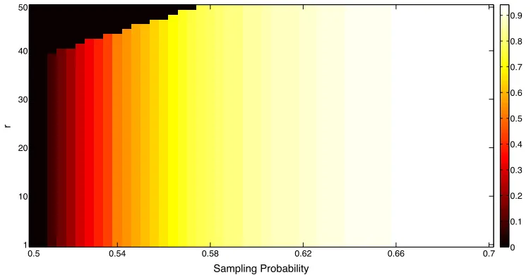
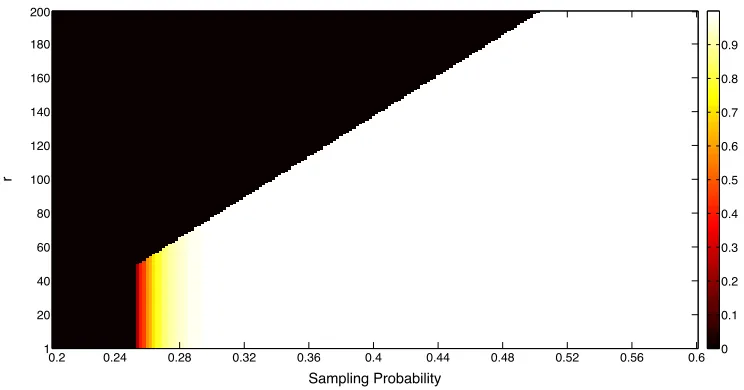
In Fig. 1 and Fig. 2, the x-axis represents the sampling probability, and the y-axis denotes the value of r. The color scale represents the lower bound on the probability of event r ∈ SΩ. For

example, as we can observe in Fig. 1, for anyr ∈ {1, . . . ,44}we haver ∈ SΩwith probability at

least0.6(approximately based on the color scale since the corresponding points are orange) given thatp= 0.54.

We consider the sampled matrixU ∈_R300×15000_{andU ∈}

R1200×240000in Fig. 1 and Fig. 2, respectively. In particular, for fixed values of sampling probabilitypandr, we first find a “small” that (15) holds by trial-and-error. Then, according to Proposition 11, we conclude that with proba-bility at least(1−)

1−exp(−

√

n1

2 )

n2

,r∈ SΩ.

Sampling Probability

r

0.5 0.54 0.58 0.62 0.66 0.7

50

40

30

20

10

1 ₀

0.1 0.2 0.3 0.4 0.5 0.6 0.7 0.8 0.9

Figure 1: Probability ofr∈ S_Ωas a function of sampling probability forU∈_R300×15000_.

Sampling Probability

r

0.2 0.24 0.28 0.32 0.36 0.4 0.44 0.48 0.52 0.56 0.6 200

180

160

140

120

100

80

60

40

20

1 0

0.1 0.2 0.3 0.4 0.5 0.6 0.7 0.8 0.9

Figure 2: Probability ofr ∈ SΩas a function of sampling probability forU∈R1200×240000.

(entries are drawn according to a uniform distribution on real numbers within an interval)n1×r

matrix andr×n2matrix. Then, each entry of the randomly generated matrix is sampled uniformly

at random and independently across entries with some sampling probability p. Afterwards, we apply the nuclear norm minimization method proposed in (Candes and Recht, 2012) for matrix completion, where the non-convex objective function in (13) is relaxed by using nuclear norm, which is the convex hull of the rank function, as follows

minimize_U0_∈

Rn1×n2 kU

0_k

∗ (17)

subject to U0_Ω=UΩ,

wherekU0k∗denotes the nuclear norm ofU0. LetUˆ∗denote an optimal solution to (17) and recall thatU∗ denotes an optimal solution to (13). Since (17) is a convex relaxation to (13), we conclude thatUˆ∗ is a suboptimal solution to (13), and therefore rank(U∗)≤rank(Uˆ∗). We used the Matlab program found online (Shabat, 2015) to solve (17).

As an example, we generate a random matrix U ∈ _R300×15000 _{(the same size as the matrix}

in Fig. 1) of rank r as described above for r ∈ {1, . . . ,50} and some values of the sampling probabilityp. Then, we obtain the rank of the completion given by (17) and denote it byr0. Due to the randomness of the sampled matrix, we repeat this procedure5times. We calculate the “gap” r0−rin each of these5runs and denote the maximum and minimum among these 5 numbers bydmax anddmin, respectively. Hence, dmax anddminrepresent the loosest (worst) and tightest (best) gaps between the rank obtained by (17) and rank of the original sampled matrix over5runs, respectively. In Figs. 3–6, the maximum and minimum gaps are plotted as a function of rank of the matrix, for different sampling probabilities.

We have the following observations.

• According to Fig. 1, forp= 0.54andp= 0.58we can ensure that the rank of any completion is an upper bound on the rank of the sampled matrix orr∗ with probability at least0.6and

0 10 20 30 40 50 0

10 20 30 40 50 60

Rank of the Sampled Matrix

Gap

Maximum Gap

Minimum Gap

Figure 3: The gaps between the rank of the obtained matrix via (17) and that of the original sampled matrix forp= 0.46.

0 10 20 30 40 50

0 5 10 15 20 25

Rank of the Sampled Matrix

Gap

Maximum Gap

Minimum Gap

Figure 4: The gaps between the rank of the obtained matrix via (17) and that of the original sampled matrix forp= 0.50.

• As we can observe in Figs. 3–6, the defined gap is always a nonnegative number, which is consistent with previous observation that forp= 0.54andp= 0.58we can certify that with high probability (≥ 0.6) the rank of any completion is an upper bound on the rank of the sampled matrix orr∗.

0 10 20 30 40 50 0

1 2 3 4 5 6 7 8 9

Rank of the Sampled Matrix

Gap

Maximum Gap

Minimum Gap

Figure 5: The gaps between the rank of the obtained matrix via (17) and that of the original sampled matrix forp= 0.54.

0 10 20 30 40 50

0 1 2 3 4 5 6

Rank of the Sampled Matrix

Gap

Maximum Gap

Minimum Gap

Figure 6: The gaps between the rank of the obtained matrix via (17) and that of the original sampled matrix forp= 0.58.

3.2 CP-Rank Tensor

Let Pi denote the Lebesgue measures on Rni×r

∗

, i = 1, . . . , d. In this subsection, we assume that the sampled tensorU ∈Rn1×...×nd_{is chosen generically from the manifold of tensors of rank} r∗=rankCP(U)(wherer∗is unknown), or in other words, the entries ofUare drawn independently with respect to Lebesgue measure on the corresponding manifold. Hence, the probability measures of all statements in this subsection areP1×P2×. . .×Pd.

ConditionAr: Each row of thed-th matricization of the sampled tensor, i.e.,U(d)includes at

leastrobserved entries.

We construct a binary valued tensor calledconstraint tensorΩ˘rbased onΩand a given number

r. Consider any subtensorY ∈_Rn1×n2×···×nd−1×1_{of the tensorU. The sampled tensorU includes}

ndsubtensors that belong toRn1×n2×···×nd−1×1_{and letY}

ifor1≤i≤nddenote thesend

subten-sors. Define a binary valued tensorY˘i ∈Rn1×n2×···×nd−1×ki_{, wherek}

i=NΩ(Yi)−rand its entries

are described as the following. We can look atY˘iaskitensors each belongs toRn1×n2×···×nd−1×1. For each of the mentionedki tensors in Y˘i we set the entries corresponding to r of the observed

entries equal to1. For each of the otherkiobserved entries, we pick one of thekitensors ofY˘iand

set its corresponding entry (the same location as that specific observed entry) equal to1and set the rest of the entries equal to0. In the case thatki = 0we simply ignoreY˘i, i.e.,Y˘i =∅

By putting together all ndtensors in dimension d, we construct a binary valued tensorΩ˘r ∈ Rn1×n2×···×nd−1×K, where K = Pin=1d ki = NΩ(U) −rnd and call it the constraint tensor.

Observe that each subtensor of Ω˘r which belongs to Rn1×n2×···×nd−1×1 _{includes exactly r + 1}

nonzero entries. In (Ashraphijuo and Wang, 2017b), an example is given on the construction ofΩ˘r.

ConditionB_r:Ω˘rconsists a subtensorΩ˘0r∈Rn1×n2×···×nd−1×Ksuch thatK=r(

Pd−1

i=1ni)−

r2−r(d−2)and for anyK0 ∈ {1,2, . . . , K}and any subtensorΩ˘00_r ∈_Rn1×n2×···×nd−1×K0 _ofΩ˘0

r

we have

r

_d−1 X

i=1

fi( ˘Ω00r)

!

−min n

max n

f1( ˘Ω00r), . . . , fd−1( ˘Ω00r)

o , r

o

−(d−2)

!

≥K0, (18)

wherefi( ˘Ω00r)denotes the number of nonzero rows of thei-th matricization ofΩ˘00r.

The following lemma is a re-statement of Theorem1in (Ashraphijuo and Wang, 2017b).

Lemma 13 With probability one, there are only finitely many rank-r∗completions of the sampled tensor if and only if ConditionsA_r∗ andB_r∗hold.

Definition 14 LetS_Ωdenote the set of all natural numbersrsuch that both ConditionsA_randB_r

hold.

Lemma 15 There exists a numberrΩsuch thatSΩ ={1,2, . . . , rΩ}.

Proof The proof is similar to the proof of Lemma 3 since the dimension of the manifold of CP rank-rtensors isr(Pd

i=1ni)−r2−r(d−1), which is an increasing function inr.

The following theorem gives an upper bound on the unknown rankr∗.

Theorem 16 With probability one, exactly one of the following statements holds (i)r∗∈ SΩ={1,2, . . . , rΩ};

Proof Similar to the proof of Theorem 4, it suffices to show that the assumptionr∗ ∈ S/ _Ω results that there exists a completion of U of CP rank r, where r ∈ SΩ, with probability zero. Define

V = (V₁, . . . ,V_r)as the basis of the rank-rCP decomposition ofU as in (3), whereV_l =al₁⊗al₂⊗

. . .⊗al_d−1 ∈_Rn1×...nd−1 _{is a rank-1tensor anda}l

iis defined in (3) for1 ≤l ≤rand1 ≤i≤d.

DefineY = (a1_d, . . . ,a_dr)andV ⊗_dY =Pr

l=1Vl⊗ald. Observe thatU =

Pr

l=1Vl⊗ald=V ⊗dY.

Observe that each row ofU(d) includes at leastrΩ+ 1observed entries since ConditionArΩ

holds. Moreover, the existence of a completion of the sampled tensor U of rank r ∈ S_Ω results in the existence of a basis V = (V₁, . . . ,V_r)such that there existsY = (a1_d, . . . ,ar_d) andU_Ω = (V ⊗dY)_Ω. As a result, givenV, each observed entry ofU results in a degree-1 polynomial in

terms of the entries ofYas

U(~x) =

r

X

l=1

V_l(x1, . . . , xd−1)ald(xd). (19)

Note that rΩ ≥ r and each row of U(d) includes at least rΩ + 1 ≥ r + 1observed entries.

Considerr+ 1of the observed entries of the first row ofU(d)and we denote them byU(~x1),. . .,

U(~xr+1), where the last component of the vectorx~i is equal to one,1≤i≤r+ 1. Similar to the

proof of Theorem 4, genericity ofU results in

U(~xr+1) = r

X

l=1

tlU(~xi), (20)

wheretl’s are constant scalars,l= 1, . . . , r. On the other hand, according to Lemma 13 there exist

at most finitely many completions of the sampled tensor of rankr. Therefore, there exist a com-pletion ofUof rankrwith probability zero. Moreover, an equation of the form of (20) holds with probability zero asr∗ ≥r+ 1andU is chosen generically from the manifold of tensors of rank-r∗. Therefore, there exists a completion of rankrwith probability zero.

Corollary 17 Consider an arbitrary numberr0 ∈ S_Ω. Similar to Theorem 16, it follows that with probability one, exactly one of the followings holds

(i)r∗∈ {1,2, . . . , r0};

(ii) For any arbitrary completion of the sampled tensorU of rankr, we haver /∈ {1,2, . . . , r0}.

Corollary 18 Assuming that there exists a CP rank-rcompletion of the sampled tensorU such that

r∈ S_Ω, we conclude that with probability oner∗≤r.

Corollary 19 LetU∗ _{denote an optimal solution to the following NP-hard optimization problem}

minimizeU0_∈

Rn1×···×nd rankCP(U

0₎

(21) subject to U_Ω0 =U_Ω.

Assume thatrankCP(U∗)∈ SΩ. Then, Corollary 18 results thatr∗ =rankCP(U∗)with probability one.

Lemma 20 Assume thatn1 =n2 =· · · =nd= n,d >2,n >max{200, r(d−2)}andr ≤ n₆. Moreover, assume that the sampling probability satisfies

p > 1 nd−2max

27 logn

+ 9 log

2r(d−2)

+ 18,6r

+ √₄ 1

nd−2. (22)

Then, with probability at least(1−)1−exp(−

√

nd−2

2 )

n2

, we haver ∈ S_Ω.

The following corollary is the probabilistic version of Corollaries 18 and 19.

Corollary 21 Assuming that there exists a CP rank-rcompletion of the sampled tensorU such that the conditions given in Lemma 20 hold, with the sampling probability satisfying(22), we conclude

that with probability at least(1−)

1−exp(−

√

nd−2

2 )

n2

we haver∗ ≤r. Therefore, given that

(22)holds forr =rank(U∗)andU∗denotes an optimal solution to the optimization problem(21),

with probability at least(1−)

1−exp(−

√

nd−2

2 )

n2

we haver∗ =rank(U∗).

3.2.1 NUMERICALRESULTS

We generate a random tensor U ∈ R8×8×8×8×8×8 of CP-rank 2 by adding two random rank-1 tensors. The color scale represents the lower bound on the probability that we can guarantee the rank of a given completion is an upper bound on the true value of rank. Then, we solve the following convex optimization problem for different values of the sampling probability.

minimize_U0_∈

Rn1×···×nd kUe0₍₃₎k_∗ (23)

subject to U_Ω0 =U_Ω.

Note that rank of any of the unfoldings of a tensor is a lower bound on the CP-rank of that tensor. Hence, we minimize the nuclear norm of the unfolding with the possible maximum rank among all unfoldings as Ue₍₃₎ ∈ _R512×512. Then, we use the Matlab toolbox found online “Tensorlab” to calculate the CP-rank of the obtained tensor via solving convex program (23) (there are other methods to calculate CP decomposition, e.g., (Pimentel-Alarc´on, 2016)). In Figure 7, gap represents the CP-rank of the solution of (23) minus the CP-rank of the original sampled tensor.

4. Vector-Rank Cases

4.1 Multi-View Matrix

LetP1andP2denote the Lebesgue measures onRn×r

∗

1 and_Rr

∗

1×n1_{, respectively. Moreover, letP}

3

andP4 denote the Lebesgue measures onRn×(r

∗_−r∗

1) and_Rr

∗

2×n2_{, respectively. In this paper, we}

assume thatUis chosen generically from the manifold corresponding to rank vector(r₁∗, r₂∗, r∗), i.e., the entries ofUare drawn independently with respect to Lebesgue measure on the corresponding manifold. Hence, the probability measures of all statements in this subsection areP1×P2×P3×P4.

The following Conditions will be used frequently in this subsection.

Condition Ar1,r2: Each column of U1 and U2 include at least r1 and r2 sampled entries,

Sampling Probability

Gap

0.11 0.12 0.13 0.14 0.15 0.16 0.17 0.18 5

4

3

2

1

0

0.1 0.2 0.3 0.4 0.5 0.6 0.7 0.8 0.9

Figure 7: The rank gap as a function of sampling probability forU ∈_R8×8×8×8×8×8_{of CP-rank2.}

We construct a binary valued matrix called constraint matrix for multi-view matrix U as ˘

Ωr1,r2 = [Ω˘r1|Ω˘r2], whereΩ˘r1 andΩ˘r2 represent the constraint matrix for single-view matrices

U1 andU2(defined in Section 3.1), respectively.

ConditionBr1,r2,r:Ω˘r1,r2 consists a submatrixΩ˘

0

r1,r2 ∈R

n×K_{such thatK=nr−r}2_−r2 1−

r2

2 +r(r1+r2)and for anyK0 ∈ {1,2, . . . , K}and any submatrixΩ˘00r1,r2 ∈R

n×K0 _ofΩ˘0

r1,r2 we

have

(r−r2)

f(Ω˘00_r1)−r1

+

+ (r−r1)

f(Ω˘00_r2)−r2

+

+(r1+r2−r)

f(Ω˘00_r1,r2)−(r1+r2−r)

+

≥K0, (24)

wheref(X)denotes the number of nonzero rows ofXfor any matrixXandΩ˘00_r1,r2 = [Ω˘00_r1|Ω˘00_r2], and alsoΩ˘00_r1 andΩ˘00_r2 denote the columns ofΩ˘00_r1,r2 corresponding toΩ˘r1 andΩ˘r2, respectively.

The following lemma is a re-statement of Theorem2in (Ashraphijuo et al., 2017c).

Lemma 22 With probability one, there are only finitely many completions of the sampled multi-view data if and only if ConditionsAr₁∗,r₂∗andBr∗₁,r∗₂,r∗ hold.

Definition 23 Denote the rank vectorr = (r1, r2, r). Define the generalized inequalityr0 ras the component-wise set of inequalities, e.g.,r0₁ ≤r1,r20 ≤r2andr0 ≤r.

Definition 24 LetS_Ωdenote the set of allrsuch that both ConditionsAr1,r2 andBr1,r2,rhold.

Lemma 25 Assumer ∈ S_Ω. Then, for anyr0 r, we haver0 ∈ S_Ω.

also observe that the fact thatmax{r1, r2} ≤r≤r1+r2≤min{2n, n1+n2}implies that reducing

any of the valuesr1, r2, andrreduces the value ofrn+r1n1+r2n2−r2−r21−r22+r(r1+r2).

Hence, the dimension of the manifold corresponding to rank vector r is larger than that for rank vectorr0, givenr0 r, and thus similar to the proof of Lemma 3, finite completability of data with rresults finite completability of data withr0with probability one. Then, using Lemma 22, the proof is complete.

The following theorem provides a relationship between the unknown rank vectorr∗andS_Ω.

Theorem 26 With probability one, exactly one of the following statements holds (i)r∗∈ S_Ω;

(ii) For any arbitrary completion of the sampled matrixUof rank vectorr, we haver /∈ SΩ.

Proof Similar to the proof of Theorem 4, suppose that there does not exist a completion ofUof rank vectorrsuch thatr ∈ SΩ. Therefore, it is easily verified that statement (ii) holds and statement

(i) does not hold. On the other hand, assume that there exists a completion ofU of rank vectorr, wherer∈ SΩ. Hence, statement (ii) does not hold and to complete the proof it suffices to show that

with probability one, statement (i) holds. Similar to Theorem 4, we show that assumingr∗ ∈ S/ Ω,

there exists a completion ofUof rank vectorr, wherer∈ S_Ω, with probability zero.

Sincer∗ ∈ S/ _Ω, according to Lemma 25, for anyr ∈ S_Ωat least one the following inequalities holds; r1 < r∗1, r2 < r∗2 andr < r∗. Note that assuming that there exists a completion ofU1

of rankr1 with probability zero results that there exists a completion of U of rank vectorr with

probability zero and similar statement holds forr2andr. Hence, in any possible scenario (r1 < r1∗

orr2 < r∗2 orr < r∗) the similar proof as in Theorem 4 (for single-view matrix) results that there

exists a completion ofUof rank vectorr, wherer ∈ S_Ω, with probability zero.

Corollary 27 Consider a subsetS_Ω0 ofSΩsuch that for any two members ofSΩthatr0 r00and

r00∈ S0

Ωwe haver0 ∈ SΩ0 . Then, with probability one, exactly one of the followings holds

(i)r∗∈ S0

Ω;

(ii) For any arbitrary completion ofUof rank vectorr, we haver /∈ S_Ω0 .

Proof Note that the property in the statement of Lemma 25 holds forS_Ω0 as well asSΩ. Moreover,

asS_Ω0 ⊆ S_Ω, for anyr∈ S_Ω0 there exists at most finitely many completions ofUof rank vectorr, and therefore the rest of the proof is the same as the proof of Theorem 26.

Corollary 28 Assuming that there exists a completion ofUwith rank vector rsuch thatr ∈ S_Ω, then with probability oner∗ r.

The following lemma which is a re-statement of Theorem3in (Ashraphijuo et al., 2017c) gives the number of samples per column that is needed to ensure that ConditionsAr1,r2 andBr1,r2,rhold

Lemma 29 Suppose that the following inequalities hold

n

6 ≥ max{r1, r2,(r1+r2−r)}, (25)

n1 ≥ (r−r2)(n−r1), (26)

n2 ≥ (r−r1)(n−r2), (27)

n1+n2 ≥ (r−r2)(n−r1) + (r−r1)(n−r2)

+ (r1+r2−r)(n−(r1+r2−r)). (28)

Moreover assume that eachcolumnofUis observed in at leastlentries, uniformly at random and independently across entries, where

l >max

9 log

n

+ 3 log

3 max{r−r2, r−r1, r1+r2−r}

+ 6,2r1,2r2

. (29)

Then, with probability at least1−,r∈ S_Ω.

The following proposition is the probabilistic version of Theorem 26 in terms of the sampling probability instead of verifying ConditionsAr1,r2 andBr1,r2,r.

Proposition 30 Suppose that (25)-(28) hold for r and that each entry of the sampled matrix is observed uniformly at random and independently across entries with probabilityp, where

p > 1 nmax

9 logn

+ 3 log

3 max{r−r2, r−r1, r1+r2−r}

+ 6,2r1,2r2

+ √₄1

n.

Then, with probability at least(1−)1−exp(−

√

n 2 )

n1+n2

, we haver ∈ S_Ω.

Proof The proposition is easy to verify using Lemma 29 and Lemma 9 (similar to the proof for Proposition 11).

Corollary 31 Assuming that there exists a completion ofUof rank vectorrsuch that(25)-(28)hold and the sampling probability satisfies(30), then with probability at least(1−)

1−exp(−

√

n 2 )

n1+n2

we haver∗ r.

4.2 Tucker-Rank Tensor

LetPidenote the Lebesgue measures on Rni×m

∗

i_,i =j+ 1, . . . , d, and_{P0 denotes the Lebesgue} measures on Rm

∗

j+1×m∗j+2×...×m∗d_{. In this subsection, we assume that the sampled tensor} U ∈ Rn1×...×nd is chosen generically from the manifold of tensors of rank r∗ = rankTucker(U) =

(m∗_j+1, . . . , m∗_d) (where r∗ is unknown), or in other words, the entries of U are drawn indepen-dently with respect to Lebesgue measure on the corresponding manifold. Hence, the probability measures of all statements in this subsection areP0×Pj+1×Pj+2×. . .×Pd.

Without loss of generality assume that m∗_j+1 ≥ . . . ≥ m∗_d throughout this subsection. Also, givenr= (mj+1, . . . , md), define the following function

gr(x) = d

X

i=j+1

min

 

 ri,



x−

i−1

X

i0_=j+1

ri0





+ 



Definition 32 For anyi∈ {j+ 1, . . . , d}andS_i ⊆ {1, . . . , ni}, defineU(Si)as a set containing the entries of|Si|rows (corresponding to the elements ofSi) ofU(i). Moreover, defineU(Sj+1,...,Sd)=

U(Sj+1)_{∪. . .∪ U}(Sd)_.

ConditionATucker

r : There exist

Pd

i=j+1(nimi)observed entries such that for anySi ⊆ {1, . . . ,

ni}fori∈ {j+ 1, . . . , d},U(Sj+1,...,Sd)includes at mostPd_i=j+1|Si|miof the mentionedPd_i=j+1

nimiobserved entries.

LetPbe a set ofPd

i=j+1(nimi)observed entries such that they satisfy ConditionATuckerr . Now,

we construct a(j+ 1)th-order binary constraint tensorΩ˘rin some sense similar to that in Section

3.2. For any subtensorY ∈_Rn1×n2×···×nj×1×···×1 _{of the tensorU, letN}

Ω(YP)denote the number

of sampled entries inYthat belong toP.

The sampled tensorUincludesnj+1nj+2· · ·ndsubtensors that belong toRn1×n2×···×nj×1×···×1 and we label these subtensors byY_(tj+1,...,t

d)where(tj+1, . . . , td)represents the coordinate of the subtensor. Define a binary valued tensorY˘_{(tj+1,···,t}

d) ∈ R

n1×n2×···×nj×

d−j z }| {

1×. . .×1×k_{, wherek=}

NΩ(Y(tj+1,...,td))−NΩ(Y P

(tj+1,...,td))and its entries are described as the following. We can look at

˘

Y_(tj+1,···,td)asktensors each belongs toR

n1×n2×···×nj×1×···×1_{. For each of the mentionedktensors} inY˘_(tj+1,···,td)we set the entries corresponding to theNΩ(Y

P

(tj+1,...,td))observed entries that belong toP equal to1. For each of the otherkobserved entries, we pick one of thektensors ofY˘_{(tj+1,···,td)}

and set its corresponding entry (the same location as that specific observed entry) equal to1and set the rest of the entries equal to0.

For the sake of simplicity in notation, we treat tensorsY˘_{(tj+1,···,td)}as a member ofRn1×n2×···×nj×k

instead ofRn1×n2×···×nj× d−j z }| {

1× · · · ×1×k_{. Now, by putting together alln}

j+1nj+2· · ·ndtensors in

dimension (j+ 1), we construct a binary valued tensor Ω˘r ∈ Rn1×n2×···×nj×Kj, where Kj =

NΩ(U)−Pd_i=j+1(nimi)and call it theconstraint tensor(Ashraphijuo et al., 2016a). In

(Ashraphi-juo et al., 2016a), an example is given on the construction ofΩ˘r.

ConditionBTucker

r : The constraint tensorΩ˘rconsists a subtensorΩ˘0r ∈Rn1×n2×···×nj×K such

thatK =Πj_i=1ni Πdi=j+1mi

−Pd

i=j+1m2i and for anyK0 ∈ {1,2, . . . , K}and any subtensor

˘

Ω00_r ∈Rn1×n2×···×nd−1×K0 _ofΩ˘0

rwe have

Πd_i=j+1mi fj+1( ˘Ω00r)

−gr

fj+1( ˘Ω00r)

≥K0, (31)

wherefj+1( ˘Ω00r)denotes the number of nonzero columns of the(j+ 1)-th matricization ofΩ˘00r.

The following lemma is a re-statement of Theorem3in (Ashraphijuo et al., 2016a).

Lemma 33 With probability one, there are only finitely many completions of rankr∗of the sampled tensor if and only if ConditionsATucker

r∗ andBTucker_r∗ hold.

Definition 34 LetSΩ denote the set of all rank vectors r such that both Conditions ATuckerr and

BTucker

r hold.

Proof Note that the dimension of the manifold corresponding tor is

Πj_i=1ni Πdi=j+1mi

+

Pd

i=j+1nimi−

Pd

i=j+1m2i, and thus by reducing the value ofmi0 by one (fori0 ∈ {j+1, . . . , d}),

the value of the mentioned dimension reduces by at leastΠj_i=1ni

+ni−2mi+ 1, which is greater

than zero sincemi≤ni. The rest of the proof is similar to the proof of Lemma 3.

Definition 36 DefineS_Ω(r)as a subset ofS_Ω, which includes allr0∈ S_Ωthatr0 r.

The following theorem gives a relationship betweenr∗andSΩ.

Theorem 37 With probability one, exactly one of the following statements holds (i)r∗∈ S_Ω;

(ii) For any arbitrary completion of the sampled tensorU of rankr, we haver /∈ SΩ(r∗).

Proof Similar to the proof of Theorem 4, to complete the proof it suffices to show that the as-sumptionr∗ ∈ S/ _Ω results that there exists a completion of U of rankr, where r ∈ S_Ω(r∗), with probability zero. Note that r ∈ SΩ(r∗) ⊆ SΩ results that ConditionsATuckerr and BrTucker hold.

Moreover, note thatr r∗and since r∗ ∈ S/ _Ω we conclude that there existsi0 ∈ {j+ 1, . . . , d}

such thatmi0 < m

∗

i0. As a result,

Pd

i=j+1nimi <Pdi=j+1nim∗i.

ConditionBTucker

r ensures there exists at least one more observed entry (otherwise the constraint

tensor does not exist) besides thePd

i=j+1nimi mentioned observed entries. Given the basisC ∈ Rn1×...×nj×mj+1×...×md as in (7), there existPdi=j+1nimi variables in the corresponding Tucker

decomposition. However, we have Pd

i=j+1nimi + 1 polynomials in terms these Pdi=j+1nimi

variables and therefore the last polynomials can be written as algebraic combination of the other Pd

i=j+1nimi polynomials. This leads to a linear equation in terms of the

Pd

i=j+1nimi+ 1

cor-responding observed entries. On the other hand, the Pd

i=j+1nimi observed entries satisfy the

property stated as ConditionATucker

r and it is easily verified that there exist

Pd

i=j+1nim∗i entries

(observed and non-observed) satisfying Condition ATucker

r∗ such that the union of the mentioned

Pd

i=j+1nimi entries with any arbitrary other observed entry be a subset of those Pdi=j+1nim∗i

entries. However, U is generically chosen from the manifold corresponding tor∗ and therefore a particular linear equation in terms of the mentionedPd

i=j+1nim

∗

i entries holds with probability

zero. The rest of the proof is similar to the proof of Theorem 4.

Corollary 38 Assuming that there exists a completion ofU with rank vectorrsuch thatr ∈ SΩ, we conclude that with probability oner∗r.

The following lemma is Corollary2 in (Ashraphijuo et al., 2016a), which ensures that Condi-tionsATucker

r andBrTuckerhold with high probability.

Lemma 39 Assume that Pd

i=j+1m2i ≤ Πdi=j+1mi, Πdi=j+1ni ≥ NjΠdi=j+1mi −Pdi=j+1m2i,

probabilityp, where

p > 1 Nj

6 log (Nj) + 2 log max

(

2Pd

i=j+1r2i

,

2Πd_i=j+1ri−2Pdi=j+1ri2

)!

+ 4

!

+ 1

4

p Nj

.

Then, with probability at least(1−) 1−exp(−

q Πj_i=1ni

2 )

!Πd_i=j+1ni

,r∈ S_Ω.

The following corollary is the probabilistic version of Theorem 37.

Corollary 40 Assuming that there exists a completion of the sampled tensorU of Tucker rankr

such that the assumptions in Lemma 39 hold and the sampling probability satisfies(32), then with

probability at least(1−) 1−exp(−

q Πj_i=1ni

2 )

!Πd_i=j+1ni

we haver∗r.

4.2.1 NUMERICALRESULTS

We generate a random tensor U ∈ _R8×8×8×8×8×8 _{of Tucker-rank(1,3,3,2,2). The color scale}

represents the lower bound on the probability that we can guarantee the rank of a given completion is a component-wise upper bound on the true rank. Then, we solve the following convex optimization problem for different values of the sampling probability.

minimize_U0_∈

Rn1×···×nd k

d

X

i=1

U0_(i)k∗ (32)

subject to U_Ω0 =U_Ω.

Then, we calculate rank of each matricization of the tensor obtained via solving (32) to find its Tucker-rank. In this scenario, for each component of the Tucker-rank, we find the percentage of error via mi−m∗i

n−m∗_i ×100%, wheren = 8, mi andm

∗

i are thei-th rank component of the obtained

tensor and original tensor, respectively. Hence,100% error simply means that the corresponding matricization is full rank. In Figure 8, gap represents the average of the defined error over all components of Tucker-rank, i.e., over all matricizations.

4.3 TT-Rank Tensor

Let Pi denote the Lebesgue measures on Ru

∗

i−1×ni×u∗i_{, i = 1, . . . , d, where u}∗

0 = u∗d = 1. In

this subsection, we assume that the sampled tensor U ∈ _Rn1×...×nd _{is chosen generically from} the manifold of tensors of rankr∗ = rankTT(U) = (u∗₁, . . . , u∗_d−1) (wherer∗ is unknown), or in other words, the entries of U are drawn independently with respect to Lebesgue measure on the corresponding manifold. Hence, the probability measures of all statements in this subsection are P1×. . .×Pd.

ConditionATT

r : Each row of thed-th matricization of the sampled tensor, i.e.,U(d)includes at

leastud−1observed entries.

We construct thed-way binary valued constraint tensorΩ˘ud−1 similar to that in Section 3.2 as

Sampling Probability

Gap (%)

0.13 0.132 0.134 0.136 0.138 0.140 0.142 0.144 0.146 0.148 0.15

100

90

80

70

60

50

40

30

20

10

0 0

0.1 0.2 0.3 0.4 0.5 0.6 0.7 0.8 0.9

Figure 8: The rank gap as a function of sampling probability forU ∈R8×8×8×8×8×8of Tucker-rank

(1,3,3,2,2).

U includesndsubtensors that belong toRn1×n2×···×nd−1×1and letYi for1≤i≤nddenote these

ndsubtensors. Define a binary valued tensorY˘i ∈Rn1×n2×···×nd−1×ki, whereki =NΩ(Yi)−ud−1

and its entries are described as the following. We can look at Y˘_i aski tensors each belongs to Rn1×n2×···×nd−1×1_{. For each of the mentionedk}

itensors inY˘i we set the entries corresponding to

ud−1of the observed entries equal to1. For each of the otherkiobserved entries, we pick one of the

kitensors ofY˘i and set its corresponding entry (the same location as that specific observed entry)

equal to1and set the rest of the entries equal to0. In the case thatki = 0we simply ignoreY˘i, i.e.,

˘ Y_i =∅

By putting together allndtensors in dimensiond, we construct a binary valued tensorΩ˘ud−1 ∈

Rn1×n2×···×nd−1×K_{, where K =} Pnd

i=1ki =NΩ(U)−ud−1ndand call it theconstraint tensor.

Observe that each subtensor ofΩ˘ud−1 which belongs toR

n1×n2×···×nd−1×1_{includes exactlyu}

d−1+1

nonzero entries. In (Ashraphijuo and Wang, 2017a), an example is given on the construction of

˘ Ωud−1.

ConditionBTT

r :Ω˘ud−1 consists a subtensorΩ˘

0

ud−1 ∈R

n1×n2×···×nd−1×K_{such thatK =}Pd−1

i=1

ui−1niui−

Pd−1

i=1 u2i and for anyK0 ∈ {1,2, . . . , K}and any subtensorΩ˘00ud−1 ∈R

n1×n2×···×nd−1×K0

ofΩ˘0_u

d−1 we have

d−1

X

i=1

ui−1fi( ˘Ω00ud−1)ui−u

2 i

+

≥K0, (33)

wherefi( ˘Ω00ud−1)denotes the number of nonzero rows of thei-th matricization ofΩ˘

00

ud−1.

The following lemma is a re-statement of Theorem1in (Ashraphijuo and Wang, 2017a).

Lemma 41 With probability one, there are only finitely many completions of rankr∗of the sampled tensor if and only if ConditionsATT

r∗ andBTT_r∗ hold.

The following lemma will be used in Lemma 44.

Lemma 43 ui≤min{ui−1ni, ui+1ni+1}for1≤i≤d−1.

Proof We first show that ui ≤ ui−1ni, which is easily verified for i = 1as Ue₁ includes n₁ rows and u0 = 1, and therefore assume that i > 1. Define the (d− 1)-way tensor Uli ∈ Rn1×...×ni−1×ni+1×...×ndsuch thatUli(x1, . . . , xi−1, xi+1, . . . , xd) =U(x1, . . . , xi−1, li, xi+1, . . . ,

xd) for 1 ≤ i ≤ dand 1 ≤ li ≤ ni. Also, recall that Uel₍i_i−1) denotes the (i−1)-th unfold-ing of Uli_{. Observe that Ue}li

(i−1) is a subset of columns of matrix Ue(i−1) (those columns that

correspond to the entries of U with the i-th component of the location equal to li). Therefore,

rank(Uel₍i_i−1))≤rank(Ue_(i−1)) =u_i−1.

On the other hand, observe that Uel₍i_i−1) is a subset of rows of Ue_(i) (those rows that corre-spond to the entries of U with thei-th component of the location equal toli). Hence, the union

of rows of Ueli

(i−1)’s for 1 ≤ li ≤ ni constitute all rows ofUe(i). Therefore,ui = rank(Ue(i)) ≤

Pni

li=1rank(Ue

li

(i−1))≤niui−1. Similarly, we can show thatui ≤ui+1ni+1to complete the proof.

Lemma 44 Assumer ∈ SΩ. Then, for anyr0 r, we haver0 ∈ SΩ.

Proof Note that the dimension of the manifold corresponding torisPd

i=1ui−1niui−Pdi=1−1u2i.

If we reduce the value of ui by one, the value of the mentioned dimension reduces by ui−1ni+

ui+1ni+1−2ui+ 1. According to Lemma 43,ui−1ni+ui+1ni+1−2ui+ 1is greater than zero,

and thereforer0 r results that the dimension of the manifold corresponding tor is greater than that corresponding tor0. The rest of the proof is similar to the proof of Lemma 3.

Definition 45 DefineSˆΩ as the set of all rank vectorsr ∈ SΩ such that there exists a rank vector

r0 ∈ S_Ωwithr r0 andud−1 < u0d−1 (instead ofud−1 ≤ u0d−1). Note thatSˆΩ also satisfies the property in Lemma 44.

Theorem 46 With probability one, exactly one of the following statements holds: (i)r∗∈Sˆ_Ω;

(ii) For any arbitrary completion of the sampled tensorU of rankr, we haver /∈Sˆ_Ω.

Proof Similar to the proof of Theorem 4, to complete the proof it suffices to show that the assump-tionr∗ ∈/ Sˆ_Ωresults that there exists a completion ofU of rankr, wherer ∈Sˆ_Ω, with probability zero. Define the multiplicationU(1)_{. . .U}(d−1)_{in (9) as the basis of the rankrTT decomposition of}

U. Then, by considering the(d−1)-th unfolding ofU(1)_{. . .U}(d−1)_{in TT decomposition we obtain}

a matrix factorization of the(d−1)-th unfolding ofU. The rest of the proof is similar to the proof of Theorem 4.

Corollary 47 Consider a subsetSˆ0

ΩofSˆΩsuch that for any two members ofSˆΩ thatr00 r0and

r0 ∈Sˆ0

Ωwe haver00∈SˆΩ0 . Then, with probability one, exactly one of the followings holds (i)r∗∈Sˆ0

Ω;

(ii) For any arbitrary completion ofU of rank vectorr, we haver /∈Sˆ_Ω0 .

Corollary 48 Assuming that there exists a completion ofU with rank vectorrsuch thatr ∈SˆΩ, we conclude that with probability oner∗r.

The following lemma is Lemma 14 in (Ashraphijuo and Wang, 2017a), which ensures that ConditionsATT

r andBTTr hold with high probability.

Lemma 49 Definem=Pd−2

k=1uk−1uk,M =nPdk−=12uk−1uk−Pkd−=12u2kandu0 = max

n

u1

u0, . . . ,

ud−2

ud−3

o

. Assume thatn1 =n2 =· · ·=nd=n,n >max{m,200}andu0 ≤min{n₆, ud−2}hold. Moreover, assume that the sampling probability satisfies

p > 1 nd−2max

27 log

n

+ 9 log

2M

+ 18,6ud−2

+ √₄ 1

nd−2. (34)

Then, with probability at least(1−)1−exp(−

√

nd−2

2 )

n2

, we haver ∈ S_Ω.

The following corollary is the probabilistic version of Corollary 48.

Corollary 50 Assuming that there exists a completion of the sampled tensorU of TT rankr such that the assumptions in Lemma 49 hold and the sampling probability satisfies(34), then with

prob-ability at least(1−)

1−exp(−

√

nd−2

2 )

n2

we haver∗r.

4.3.1 NUMERICALRESULTS

We generate a random tensorU ∈R8×8×8×8×8×8 of TT-rank(1,2,4,1,1). The color scale repre-sents the lower bound on the probability that we can guarantee the rank of a given completion is a component-wise upper bound on the true rank. Then, we solve the following convex optimization problem for different values of the sampling probability.

minimize_U0_∈

Rn1×···×nd k

d−1

X

i=1

e

U0_(i)k∗ (35)

subject to U_Ω0 =UΩ.

Then, we calculate rank of each unfolding of the tensor obtained via solving (35) to find its TT-rank. In this scenario, for each component of the TT-rank, we find the percentage of error via ui−u∗i

min{ni_,nd−i_}−u∗

i

×100%, where n = 8, d = 6, ui and u∗i are the i-th rank component of

Sampling Probability

Gap (%)

0.12 0.125 0.13 0.135 0.14 0.145 0.15 0.155 0.16 0.165 0.17

100

90

80

70

60

50

40

30

20

10

0 0

0.1 0.2 0.3 0.4 0.5 0.6 0.7 0.8 0.9

Figure 9: The rank gap as a function of sampling probability forU ∈ R8×8×8×8×8×8 of TT-rank

(1,2,4,1,1).

5. Conclusions

We make use of the recently developed algebraic geometry analyses that study the fundamental conditions on the sampling patterns for finite completability under a number of low-rank matrix and tensor models to treat the problem of rank approximation for a partially sampled data. Particularly, the goal is to approximate the unknown scalar or vector rank based on the sampling pattern and the rank of a given completion. A number of data models have been treated, including single-view matrix, multi-single-view matrix, CP tensor, tensor-train tensor and Tucker tensor. First we have provided an upper bound on the unknown scalar rank (for single-view matrix and CP tensor) and an component-wise upper bound on the vector rank (for multi-view matrix, Tucker tensor and TT tensor) with probability one assuming that the sampling pattern satisfies the proposed combinatorial conditions. Moreover, we have also provided probabilistic versions of such bounds that hold with high probability assuming that the sampling probability is above a threshold. In addition, for single-view matrix and CP tensor, these upper bounds can be exactly equal to the unknown scalar rank given the lowest-rank completion. To illustrate how tight our proposed upper bounds are, we have provided some numerical results for the single-view matrix case in which we applied the nuclear norm minimization to find a low-rank completion of the sampled data and observe that the proposed upper bound is almost equal to the true unknown rank.

Acknowledgments

This work was supported in part by the U.S. National Science Foundation (NSF) under grant CIF1064575, and in part by the U.S. Office of Naval Research (ONR) under grant N000141410667.

References

2017a.

Morteza Ashraphijuo and Xiaodong Wang. Fundamental conditions for low-CP-rank tensor com-pletion. Journal of Machine Learning Research, 18 (63):1–29, 2017b.

Morteza Ashraphijuo and Xiaodong Wang. Scaled nuclear norm minimization for low-rank tensor completion. arXiv preprint:1707.07976, 2017c.

Morteza Ashraphijuo, Ramtin Madani, and Javad Lavaei. Inverse function theorem for polynomial equations using semidefinite programming. InIEEE 54th Annual Conference on Decision and Control (CDC), pages 6589–6596, 2015.

Morteza Ashraphijuo, Vaneet Aggarwal, and Xiaodong Wang. Deterministic and probabilistic con-ditions for finite completability of low rank tensor. arXiv preprint:1612.01597, 2016a.

Morteza Ashraphijuo, Ramtin Madani, and Javad Lavaei. Characterization of rank-constrained feasibility problems via a finite number of convex programs. In2016 IEEE 55th Conference on Decision and Control (CDC), pages 6544–6550, 2016b.

Morteza Ashraphijuo, Ramtin Madani, and Javad Lavaei. Characterization of rank-constrained fea-sibility problems via a finite number of convex programs. InIEEE 55th Conference on Decision and Control (CDC), pages 6544–6550, 2016c.

Morteza Ashraphijuo, Vaneet Aggarwal, and Xiaodong Wang. A characterization of sampling pat-terns for low-Tucker-rank tensor completion problem. In IEEE International Symposium on Information Theory (ISIT), pages 531–535, 2017a.

Morteza Ashraphijuo, Xiaodong Wang, and Vaneet Aggarwal. A characterization of sampling pat-terns for low-rank multi-view data completion problem. In IEEE International Symposium on Information Theory (ISIT), pages 1147–1151, 2017b.

Morteza Ashraphijuo, Xiaodong Wang, and Vaneet Aggarwal. Deterministic and probabilistic con-ditions for finite completability of low-rank multi-view data. arXiv preprint:1701.00737, 2017c.

Morteza Ashraphijuo, Xiaodong Wang, and Vaneet Aggarwal. An approximation of the CP-rank of a partially sampled tensor. In55th Annual Allerton Conference on Communication, Control, and Computing (Allerton), 2017d.

Jian Feng Cai, Emmanuel J Cand`es, and Zuowei Shen. A singular value thresholding algorithm for matrix completion. SIAM Journal on Optimization, 20(4):1956–1982, 2010.

Emmanuel Candes and Benjamin Recht. Exact matrix completion via convex optimization. Com-munications of the ACM, 55(6):111–119, 2012.

Emmanuel J Cand`es and Benjamin Recht. Exact matrix completion via convex optimization. Foun-dations of Computational Mathematics, 9(6):717–772, 2009.