Active Contour Segmentation using Level Sets

Active Contour Segmentation using Level Sets

R.Baskaran

#

Aassociate Professor , Department of Mathematics Government Arts College or women, Nilakottai, Tamil Nadu , India

Abstract A new frame work for accurate extraction of object boundary from back ground for cell nucleus segmentation of cervical cancer images is proposed in this work. This method is a new region grid algorithm for the fast evolution of level-set-based geometric active contours and compares it with other established numerical schemes. Geometric active contour models are very popular partial differential equation-based tools in object boundary extraction. This algorithm overcomes the drawback associated with the implementation of implicit schemes. The proposed system is more accurate compared with alternate split schemes. The region grid is formed by image gradient magnitude and directional information. The combined algorithm allows for the rapid evolution of the contour and convergence to its final configuration after very little iteration. The experiments demonstrate the efficiency and accuracy of the method.

Keywords — Active contour, Level set, Segmentation parametric method, Geometric method..

I. INTRODUCTION

The solution of the image segmentation problem is best described by a closed curve in the 2-D domain representing the boundary of the object. This problem can be solving by curve evolution or active contours: starting with an initial curve and evolving it to the ‟correct‟ steady state, ie. Object boundaries. This has led to various ideas, such as marker-points, volume of fluid method, cell method and, the level set method. This method utilizes the level set technique of curve treatment and more importantly, overcomes several difficulties arising in previous methods of image segmentation. Most part of this report follows that of Chan and Vase [1].

Active contours are curves that deform within digital images to recover object shapes [2]. They are classified as either parametric active contours [34]or geometric active contours [3,4] according to their representation and implementation. In particular, parametric active contours are represented explicitly as parameterized curves [5] in a Lagrangian formulation. Geometric active contours are represented implicitly as level sets of two dimensional distance functions [1,2] which evolve according to an Eulerian formulation. These two main classifications are based on the theory of curve evolution implemented using level set techniques.

.

II. MATERIALS AND METHODS A. Level Set Models

Level set theory, a formulation to implement active contours, was proposed by Osher and Sethian and it is used with level set function without re-initiation procedure by Chumming Li [6]. They represented a contour implicitly via a two-dimensional Lipschitz-continuous function Ф(x, y) :Ω R defined on the image plane. The function Ф(x, y) is called level set function, and a particular level, usually the zero level, of Ф (x, y) is defined as the contour, such as

C = {(x, y) : Ф (x, y) = 0}, ¥ (x, y) € Ω ……….( 1)

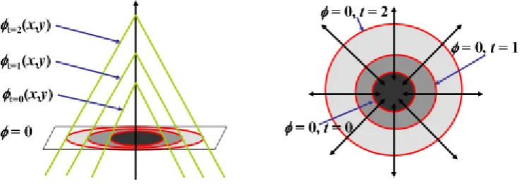
where Ω denotes the entire image plane. Figure 1(a) shows the evolution of level set function θ(x, y), and figure 1.(b) shows the propagation of the corresponding contours C. As the level set function Ф (x,y) increases from its initial stage, the corresponding set of contours.i.e. the red contour, propagates toward outside.2 With this definition, the evolution of the contour is equivalent to the evolution of the level set function, i.e. dC/dt = dθ(x, y)/dt. The advantage of using the zero level is that a contour can be defined as the border between a positive area and a negative area, so the contours can be identified by just checking the sign of Ф(x, y). The initial level set function ɸ(x, y) : ΩR may be given by the signed distance from the initial contour such as,

 0(x,y)













 



_N

_C



t y x

0 ,

, ,

0 : ,

 



 

Fig 1: Level set evolution and the corresponding contour propagation (a) topological view of level set Ф (x, y) evolution, (b) the changes on the zero

level set C : Ф (x, y) = 0

where ±D(a, b) denotes a signed distance between a and b, and Nx,y(C0) denotes the nearest neighbor pixel on initial contours C0 = C(t = 0) from (x, y). Figure 3.3(a) shows an example of initial contours C0, and figure 3.3(b) shows the initial level set function Ф0(x, y) as the signed distance computed from the initial contour C0. Ф0(x, y) increases, i.e. become brighter,

(a) (b)

Fig 2. Initial contours and corresponding signed distance

(a) the initial contour C0,( b) the initial level set function Ф0(x, y) determined by the signed distance ±D((x, y),Nx,y(C0))

As a pixel (x, y) is located further inwards from the initial contours C0, while ɸ0(x, y) decreases, i.e. become darker, as the pixel is located further outwards from the initial contours. The initial level set function is zero at the initial contour points given by, ɸ0(x, y) = 0, ¥(x, y) € C0.

The deformation of the contour is generally represented in a numerical form as a PDE. A contour evaluation can be formulated using the magnitude of the gradient vector ɸ(x, y) was formally proposed by Osher and Sethian given by the equation 3.











 

 



y x

, ,

,

  



 

  

--- (3)

Where ע denotes a constant speed term to push or pull the contour, k(·) : Ω R denotes the mean curvature of the level set function Ф(x, y) given by









    

  

  

   x y div

k , ……….……….(4)

An important characteristic of level set methods is that contours can split or merge depends on the topology of the level set function. Therefore, level set methods can detect more than one boundary simultaneously, and multiple initial contours can be placed. Figure 3(a) shows an example of the topological changes on a level set function, while figure 3(b) shows how the initially separated contours merge as the topology of level set function varies. This flexibility and convenience provide a means for an autonomous segmentation by using a predefined set of initial contours. The computational cost of level set methods is high because the computation should be done on the same dimension as the image plane Ώ. Thus, the convergence speed is relatively slower than other segmentation methods, particularly local filtering based methods. The high computational cost can be compensated by using multiple initial contours.

(a) (b)

Fig 3. The change of topology observed in the evolution of level set function and the propagation of corresponding contours: (a) the topological view of level set Ф(x, y) evolution,(b) the changes on the zero level

set C : Ф(x, y) = 0

The use of multiple initial contours increases the convergence speed by cooperating with neighbor contours quickly. Level set methods with faster convergence, called fast marching methods [14], have been studied intensively for the last decade. Because of these attractive properties, we implement the proposed active contour model using the level set method.

B. Traditional Active Contour Model

Active contours are curves that deform within digital images to recover object shapes [2]. They are classified as either parametric active contours ([6]) or geometric active contours ([3]) according to their representation and implementation. In particular, parametric active contours are represented explicitly as parameterized curves [7] in a Lagrangian formulation. Geometric active contours are represented implicitly as level sets of two dimensional distance functions [5] which evolve according to an Eulerian formulation. They are based on the theory of curve evolution implemented via level set techniques.

The first snake model was proposed by Kass [5] in 1987. The energy functional which the snake was to minimize in order to achieve equilibrium was defined as followings

Total energy of the snake E energy = E internal + E external

Here E internal represents the internal energy of the curve as bending function and E external represents the image forces pushing the snake toward the desired object. The proposed energy model was defined as

ds s X E s

X s

X

E 1/2( | '( )| | "( )| ) ext( ( ))

2 2

1

0

 



_

Since the object in interest should be recognized by the snake as a set of low values on the negative edge map, i.e. spatial gradient magnitude, the model for the image energy was defined as

E_ext1 (x, y)   |I(x,y) |2 ………..(6)

E_ext2 (x,y)   |(G_ (x,y)*I(x,y)) |2 ………(7)

Here E1 and E2 are defined with simple negative edge function and smoothening edge function with Gaussian smoothening filter where Gζ denotes a Gaussian smoothing filter with the standard deviation ζ, and λ is a suitably chosen constant. Solving the problem of snakes is to find the contour C that minimizes the total energy term E with the given set of weights α, β, and λ. In numerical experiments, a set of snake points residing on the image plane are defined in the initial stage, and then the next position of those snake points are determined by the local minimum E. The connected form of those snake points is considered as the contour.

obtain using active contour models. Depends on the contrast of the image the number iterations are increased to get the object boundary.

(a) Cancer cell hsil output of active contour result with 500 iterations

(b) Cancer cell Cyto image contour result after 500 iterations

(c) Natural image contour after 500 iterations

Fig 5. The active contour results of geometric levelset segmentation

If initial contour assumption is closed to the object boundary then the accurate object boundary can be obtain using active contour models. Depends on the contrast of the image the number iterations are increased to get the object boundary.

III. PROPOSED SYSTEM

Region grid method employ a hierarchy of grids with different sizes depends on the object present in

Fig 6. Process block diagram

A. The Level-Set Method and Active Contour Methods

An image U can be defined as a bounded real positive function on some (rectangular) domain Ω є R2 . Let its boundary be denoted θ Ω. Typically, in image processing, u є {0, 1 . . . 255}, and referred to as a grayscale image. We denote C : [0, 1]  Ω a curve parameterized by arc length. We assume C is piecewise C([0, 1]). Although the problem of image segmentation has various forms, we will consider the simplest case where we “segment” the image into two regions.

A conventional approach in solving image segmentation is to start with some initial guess C (0) = C0 and evolve C (t) in a time dependent PDE

Ct = F(C (t)) ………...……..(9)

Such that C „= lim t_ ∞ C (t) solves the problem. In other words, ideally, the model should reach a steady state when C (t) is at the correct solution. Image segmentation problems were treated in tandem with edge-detecting problems

The edge is detected by the following function

………..….(10)

For Images with distinct boundary b, ie.

For and

………(11)

It is plausible to evolve C until it “hits” points of large derivative. One such model is the following geometric active contour PDE:

……….……(12)

Where u0 is the original image and g is an edge-function. Note its similarity to the motion by mean curvature equation; the ע term, when large enough, enforces C to evolve inwards even when k= 0. The evolution should stop when C (t) = {x : g(| ▲u0(x)|) <є } for some є small.

B. Selection of Region Grid Components

All the active contour methods start with initial contour assumption based on the interactive user input or automatic region selection. The convergence process highly depends on the contour assumption or the control points. This can be used in implicit scheme as well as explicit scheme. The initial contour if it takes in general then it will take minimum of 200 to 300 iterations needed for the contour convergence. In multi-grid geometric contour model [13] they defined multi-grid approach to reduce the number of iterations. But it is not suitable for pure implicit or explicit schemes.

Input

Imag

e

Edge

indicator

function

Gradient

vector

values

Dirac

function

Snake energy

minimization

Object

contour

Result

Automatic

Initial level

set function

ROI

(x0 u x

u  



b

x    

b

x₀  

           

 g u v

t ( 0 ) .( )

  

The costly procedures of re-initialization process in active contour models are overcome variational level set approach. Our proposed scheme first define the grid based on the object present in the image, so that contour convergence takes place with minimal iterations to make the contour segmentation process efficient, accurate and without time delay.

C. Region of Interest

Based onthe reference [10] the image can be extracted using gradient information and Convergence Index

Filter (COIN). The object boundary can be extracted using gradient magnitude .And directional formulation can be extracted using COIN filter. By eliminating the force field of positive and negative values, the resultant is a closed boundary of object reference. This object reference area is used in the construction of Automatic Region Grid.

In traditional level set function, it is necessary to initialize the value of Ф0 as signed distance function. Here the variational formulation [8] without reinitialization procedure can be used. So the level set function Ф is no longer required to be initialized as a signed distance function. Let Ω0 be the sub set in the image domain Ω. The initial function Ф0 is defined by

Ф0 (x,y) = { -C for inside the boundary 0 for on the boundary C for outside the boundary } Where C > 0 is a constant.

D. Numerical scheme of Dirac function

The regularized Dirac δε(x) with є = 1.5 is used for all the experiments in this paper. Because of the diffusion term introduced by our penalizing energy, no longer need the upwind scheme [4] as in the traditional level set methods. Instead, all the spatial partial derivatives ∂Ф/∂x and ∂Ф/∂yare approximated by the central difference, and the temporal partial derivative ∂Ф/∂t is approximated by the forward difference. The approximation of (10) by the above difference scheme can be simply written as

………(13)

Where L (Фi,j) is the approximation of the right hand side in (10) by the above spatial difference scheme. The difference equation (12) can be expressed as the following iteration

,

(

)

i





L









E. Selection of Time step

The time step value plays important role in the level set function. In traditional level set function the time step has been chosen as a small value to get an accurate boundary formation. But with a small time step object convergence takes place with large number of iterations which is a time consuming process. If the selection of a big time step η =50.0 then that results minimal number of iterations for the convergence of actual contour. In this proposed method used a small time step with less number of iterations for the convergence of object boundary.

F. Level-set Formulation

Introduce a level-set function Ф such that C = {x є Ω: Ф(x) = 0}. Define the inside and outside of C by inside(C) = = {x є Ω: Ф(x) < 0}. And outside(C) = = {x є Ω: Ф(x) = 0}.

The definition of the Heaviside function H(s) to be 1 if s greater than equal to 0. Otherwise H(s) =0 if s less than 0.

G. Functional Minimization

As stated in the model definition, we seek to minimize (11). From variation calculus, the Minimization of a functional asks for the Euler-Lagrange equation to be solved. Note that, in processing with solving the Euler-Lagrange equation, the Heaviside and delta functions must be regularized to Hє and δ є so that ▲ Hє(x) = δє(x) in the strict sense of the derivative. The regularized version of the functional (5) becomes

dx c u H dx c u H dx H v

F









            2 2 0 2 1 1 0

1 ( ) (1 ( ))

) ( ) ( ) (  _  _   _   _   ……….(15) The zero level-set of Ф at the steady state is the curve C which solves the segmentation problem.

IV ALGORITHM AND EXPERIMENTAL RESULTS

Themethod can be applied for various cervical cytology images such as hsil,lsil,endo and cyto images.

The preprocessing of regional classification is carried out. After that the resultant object boundary is extracted from gradient information. This result is act as object region grid for level set active contour extraction. This Geometric Active contour with automatic region grid approach produces accurate boundary converge results.

The detailed algorithm is shown below

Algorithm:

Step 1: get the input image

Step 2 : preprocessing - classify the input image using K-Means algorithm Step 3: get the seed center of the processed image

Step 4: Find GVF and corresponding magnitude and angle Step 5: classify the object boundary

Step 6 : Set the level set based on the object boundary as automatic region grid Step 7 : using edge indicator function set edge result as external force

Step 8: Using Dirac and Curvature function set the internal force Step 9: obtain Energy equilibrium based on internal and external energy Step10. get the resultant closed contour result.

Step11: Impose the contour on the object and get the segmented result

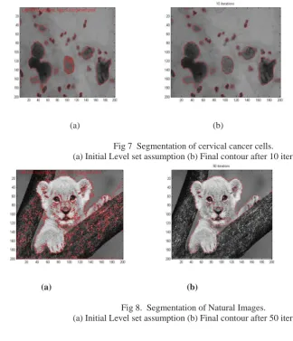
The following figure 7 shows the active boundary of cervical cell segmentation

(a) (b)

Fig 7 Segmentation of cervical cancer cells.

(a) Initial Level set assumption (b) Final contour after 10 iterations

(a) (b)

Fig 8. Segmentation of Natural Images.

V. CONCLUSION

This work focuses a novel frame work for a rapid convergence towards the boundary of geometric

active contour with variational level set formulation. Here the proposed technique gets the advantage of implicit schemes and level set approach without re-initialization procedure and fast convergence which minimize the number of iterations. So it is suitable for time critical applications. The performance of the proposed method focuses on accurate result in strong noise and weak boundaries. The experimental results shows the new region grid approach can be promising tool for all sort of applications.

REFERENCES

[1] Chan.T and L.Vase “Active contours without edges “, IEEE Transaction on Image processing Vol 10, No 2 Feb 2001. [2] Chaohan et al. “A fast Minimal path active contour model”, IEEE Transaction on Image Processing Vol 10, No 6 Jun 2001. [3] Caselles.V, F. Catte, T. Coll, and F. Dibos, “A geometric model for active contours in image processing”, Numer. Math., vol. 66, pp.

1-31, 1993.

[4] Caselles.V, R. Kimmel, and G. Sapiro, “Geodesic active contours,” International. Journal of. Computer. Vision. vol. 22, no. 1, pp. 61–79, Feb. 1997.

[5] Kass .M, A.Witkin, and D. Terzopoulos, “Snakes: Active Contour Models”, Int’l J. Comp. Vis., vol. 1, pp. 321-331, 1987

[6] Chumming Li et. al “ Level set Evaluation without reinitiation : A new variational formulation”, IEEE computer society conference CVPR 05 .

[7] Chenyang Xu and Jerry L. Prince, Gradient Vector Flow: “A New External Force for Snakes”, IEEE Proc. Conf. on Comp. Vision and Pattern Recognition (CVPR'97)

[8] Chaohan et al. “A fast Minimal path active contour model”, IEEE Transaction on Image Processing Vol 10, No 6 Jun 2001. [9] Cheng-Hung Chuang and Wen-Nung Lie, “A Downstream Algorithm Based on Extended Gradient Vector Flow Field for Object

Segmentation”, IEEE transaction on Image processing processing, vol 13 No.10 October 2004.

[10] Cheng-Hung Chuang and Wen-Nung Lie, “Automatic Multi Object Segmentation by two Phase Snake Processing”, Asian Journal of Health and Information Sciences, Vol. 1, No. 3, pp. 296-320, 2006.