Vol. 8, No. 1, March 2019, pp. 54~62
ISSN: 2252-8938, DOI: 10.11591/ijai.v8.i1.pp54-62 r 54
Distance weighted K-Means algorithm for center selection in
training radial basis function networks
Lim Eng Aik1, Tan Wei Hong2, Ahmad Kadri Junoh3
1,3Institut Matematik Kejuruteraan, Universiti Malaysia Perlis, 02600 Arau, Perlis, Malaysia. 2School of Mechatronic Engineering, Universiti Malaysia Perlis, 02600 Arau, Perlis, Malaysia.
Article Info ABSTRACT
Article history: Received Nov 27, 2018 Revised Jan 31, 2019 Accepted Feb 11, 2019
The accuracies rates of the neural networks mainly depend on the selection of the correct data centers. The K-means algorithm is a widely used clustering algorithm in various disciplines for centers selection. However, the method is known for its sensitivity to initial centers selection. It suffers not only from a high dependency on the algorithm's initial centers selection but, also from data points. The performance of K-means has been enhanced from different perspectives, including centroid initialization problem over the years. Unfortunately, the solution does not provide a good trade-off between quality and efficiency of the centers produces by the algorithm. To solve this problem, a new method to find the initial centers and improve the sensitivity to the initial centers of K-means algorithm is proposed. This paper presented a training algorithm for the radial basis function network (RBFN) using improved K-means (KM) algorithm, which is the modified version of KM algorithm based on distance-weighted adjustment for each centers, known as distance-weighted K-means (DWKM) algorithm. The proposed training algorithm, which uses DWKM algorithm select centers for training RBFN obtained better accuracy in predictions and reduced network architecture compared to the standard RBFN. The proposed training algorithm was implemented in MATLAB environment; hence, the new network was undergoing a hybrid learning process. The network called DWKM-RBFN was tested against the standard RBFN in predictions. The experimental models were tested on four literatures nonlinear function and four real-world application problems, particularly in Air pollutant problem, Biochemical Oxygen Demand (BOD) problem, Phytoplankton problem, and forex pair EURUSD. The results are compared to proposed method for root mean square error (RMSE) in radial basis function network (RBFN). The proposed method yielded a promising result with an average improvement percentage more than 50 percent in RMSE.
Keywords: Center selection Dataset size reduction K-means algorithm Neural network
Radial basis function network
Copyright © 2019 Institute of Advanced Engineering and Science. All rights reserved.
Corresponding Author: Lim Eng Aik,
Institut Matematik Kejuruteraan, Universiti Malaysia Perlis, 02600 Arau, Perlis, Malaysia. Email: e.a.lim80@gmail
1. INTRODUCTION
Radial Basis Function networks (RBFN) form a type of Artificial Neural Networks (ANNs), which has certain advantages over other kinds of ANNs, with better approximation capabilities, simpler network structures and faster learning algorithms. As a result, RBF networks turn popular among researchers. Many researchers whom have been working to produce more effective training algorithms, set alongside the standard techniques [1-7]. RBF networks are useful in approximation problems, but it requires a long time to teach the networks as it pertains to a huge number of training data, yet create a high error because of possible
invalid data or outlier in the training data. Though a combination of clustering methods in RBF networks has been proved by Sarimveis [1] to be faster in training, it still produces a more substantial error. This is due to the standard clustering algorithms, which still lack the ability to choose the most accurate and informative centers. By using distance-weighted K-means (DWKM) algorithm, we can fix the problem stated above. Noted that the more accurate the centers chosen, the more accurate the information that feeds to the train network, this leads to more accurate results. In this paper, a fast algorithm for training RBF networks which yield high accuracies is presented, where the input centers are selected through the DWKM algorithm. The methodology is illustrated through the application of eight experimental models, with four from literatures function, and four real-world problems data obtained from Lim [8]. The advantages of the presented learning strategy, DWKM-RBFN, are identified and the results are compared with standard RBFN.
2. RELATED WORKS
One of the best features of neural networks is its ability to generalize and approximate a sample data without the need of specify equation and coefficients, particularly when an unknown model describing an unknown complex relation and training data abundant. Due to their ability to generalize substantially, Radial Basis Function networks (RBFN) are usually selected for this purpose [9-21]. Furthermore, in this big data era, many domains such as image processing, text categorization, biometric, microarray, etc. had the size of datasets so large, that real-time system requires long time and memory storage to process them. Under such conditions, approximation task using available datasets can become a challenging task and difficult. This problem is more challenging in distance based learning algorithms such as RBFN [14, 22, 23], k-nearest neighbor [24-25], clustering method [21, 26-29] and support vector machine [30-32]. By default, the NN algorithm must search through all available training samples which requires large memory, and performs distance to center calculation, is slow during training of NN for approximation purposes. Additionally, due to NN stores all samples distances for training datasets, thus, noise distances are stored as well, which can cause degrade in approximation accuracy. Recently, Mirjalili [33] demonstrated that the hybrid of evolutionary algorithm such as particle swarm optimization (PSO) with RBFN shows a good performance in classification roblems and approximation problems. The used of evolutionary algorithm as a tool to select more accurate centers are also reported in many recent literatures [7, 33-38] for RBFN training indeed is a good method if the networks training speed and computation cost are not main concerns.
Along the increases of RBFN popularity, the application of RBFN in areas such as classification [10-14], pattern recognition [4, 16, 39] and prediction [15, 17-20, 40-43] increases, thus proof the wide uses and reliability of RBFN in many fields. However, RBFN accuracy mainly depending on the initial centers selected from dataset before network training begins [15, 39, 41, 44, 45]. Besides, the size of training datasets and invalid data found in datasets also play an important role in determining networks training speed and accuracy [46-50]. Furthermore, it is also reported that the learning algorithm for networks training may perform worse with the increases of dataset [51]. Hence, to solves these mentioned problems, researchers proposed the uses of clustering algorithms in centers selection [1, 28, 29, 44, 52-58] for RBFN for obtaining better accuracy and avoid possible invalid datasets includes into networks training. The most widely use clustering algorithm in centers selection is K-means algorithm, as it is the fastest, less complex algorithm, and yield good accuracy for centers selection in compared to other available clustering algorithm. However, at present available conventional clustering algorithm are not flawless algorithms that guarantee high accuracy in choosing centers. It is reported that most of conventional clustering algorithms are weak in extracting centers from series datasets [59]. Furthermore, in this work, there exist two real-world time-series datasets, the air-pollutant datasets and the forex EURUSD pair datasets. Thus, researchers further find ways to improve the weakness of existing clustering algorithms.
In recent literatures, Ismkhan [52] proposed an improved K-means algorithm with iterative multi-clustering approaches for selecting centers while minimizing the objective function. The method performed first level clustering and stored the first-generation centers, then further run the second level clustering to shorten the centers distances. This method yield good accuracy but heavy in computation cost. Similar approaches is observed in Yu et al. [53] works. Yu team uses a tri-level K-means for determining the centers. This algorithm can overcome noise and filter invalid data, but costly in computation load. The work in improving K-means algorithm was further carry-on using density concepts. Zhang et al. [28] introduced the uses of density canopy to improved K-means algorithm and yield good accuracy. The method also turn K-means algorithm become less sensitive to noise data. This method mainly focuses on calculating density of each object or data points in dataset and selected only the centers with highest density points nearby it. Similar works was found in literatures from early years [56, 60-62], using density concepts that focus on computing density of data points around the centers.
In literature by Kant and Ansari [63], introduces an initial centers selection method for K-means algorithm using Atkinson indexes. Instead of randomly selecting the initial centers for proceeding K-means
algorithm for further adjustment of centers, the authors choose to uses this approaches reduce the possible error of invalid data from randomize selection approaches. Atkinson indexes uses boundary and inequality to determine the range of centers selection for K-means algorithm. In early works by Ding et al. [64], uses similar concepts in their proposed Yinyang K-means algorithm. This algorithm uses upper and lower bounds between a point and random initial centers for selecting suitable centers. This algorithm applied a complicated process to perform the computation; it is not easily understandable for regular researcher. In addition, there were also researchers applied kernel functions for distance calculation in K-means algorithm to obtained better classification results [58]. By using kernel function, the complicated dataset are mapped into higher dimension which turning the dataset into more easily separable and classify datasets. Tzortzis and Likas [65] introduced a method to assigned weights to clusters relative to their variance. This works shed a new insight on using statistical approaches in machine learning algorithm, however it is too complicated and costly in computation. Melnykov and Melnykov [66] proposed the uses of Mahalanobis distance to replace the Euclidean distance in K-means algorithm. The approaches yield not significant improvement in accuracies.
Above literatures not focus on distance-based ratio or weightage for selecting and determine the accurate position centers. However, some literatures that focus on density of each point provided insight for our work to progress in using distance-based weight for selecting better centers for RBFN training. Using just distance-ratio as weight, the centers selection algorithm in K-means can precede faster computation without have to gone through complicated algorithm and costly computation. This paper is organized with the following section describing the standard K-means algorithm, follows by improvement done for K-means algorithm, and finally the proposed training method used for simulating and predicting the eight experimental models. Then, in section 4 discussed the results of each models and compared with standard RBFN for accuracies. Finally, section 5 concludes the findings and discussed some future work that would help in improving the proposed training method.
3. METHODOLOGY
3.1. Standard K-means algorithm
K-means (KM) algorithm [62] is one of the simplest unsupervised learning algorithms that solve the well-known clustering problem. It is an algorithm based on finding data clusters in a data set such that a cost function of dissimilarity (distance) measure is minimized. The procedure follows a simple and easy to classify with a given data set through some clusters fixed a priori. The main idea is to define K centres, one for each cluster. In other word; K-means algorithm is an algorithm to classify or group objects based on attributes or features into K number of groups. K is a positive integer number. The grouping is done by minimizing the sum squares of distances between data and the corresponding cluster centre [29, 56]. Thus, the purpose of K-means algorithm is to classify the data.
The basic step of K-means algorithm is simple: Iterate until stable (no object move group) a) Determine the centre coordinate.
b) Determine the distance of each object to the centre. c) Group the object based on minimum distance.
To describe the algorithm, we need some notations. A set of n vectors xj
∈
R
X, j = 1,…,n, are to bepartitioned into c groups Gi, i = 1,…,c. The cost function, based on the Euclidean distance between a vector
xk in group j and the corresponding cluster centre ci, is defined by:
2
1 1 ,k i
C C
i k i
i i k x G
J J x c
= = ∈
= =
⎛
⎜
−⎞
⎟
⎝
⎠
∑
∑ ∑
(1)where 2
,k i
i k i
k x G
J x c
∈
=
∑
− is the cost function within group i.The partitioned groups are defined by a c x n binary membership matrix U, where the element uij is
1, if the jth data point xj belongs to groups i and 0 otherwise. Once the cluster centres ci, are fixed, the
2 2
1, , ( _ tan )
0,
j i j k
ij
if x c x c k i Shostest dis t
U
else
− ≤ − ≠
=
⎧
⎨
⎩
(2) which means that xj belongs to group i if ci is the closest centre among all centres.
On the other hand, if the membership matrix is fixed, i.e. if uij is fixed, then the optimal centre ci that
minimizes (1) is the mean of all vectors in group i:
,
1
k i
i k
k x G i
c x
G ∈
=
∑
(3)where
G
i is the size of Gi, or 1n i j ij
G
u
=
=
∑
. The algorithm is presented below:a) Initial the cluster centre ci, i = 1,…,c. This is done by randomly selecting c point among all data points.
b) Determine membership matrix U by (2).
c) Compute the cost function according to (1). Stop if either it is below a certain tolerance value or its improvement over previous iteration is below a certain threshold. Update cluster centre according to (3). d) Repeat step 2 and 3 until convergence is achieved, until there are no more object move groups,
then stop.
Since we are not talking about the location of the centre, we need to adjust the centre location based on the current updated data. Then we assign all the data to this new centre. This process is repeated until there is no more data moving to another cluster.
3.2. Distance Weighted K-Means (DWKM) Algorithm
Typically, K-means algorithm chose its centers uniformly and randomly from vector
R
X. To reduce K-means algorithm weakness during centers selection, an improvement is made at Step 1 in Section 2.1. We proposed an improved centers selection method for K-means algorithm using distance as weightage. The improved K-means algorithm is presented as follows:1a. Select a centerc1, uniformly chosen by random from vector
R
X.1b. Assign a new center ci, chosen from vector
R
Xwith probability of2 2 1
max i i , 1, 2, 3,...,
N
k i
k
x c
i C
x c
=
−
=
−
⎛
⎞
⎜
⎟
⎜
⎟
⎜
⎟
⎝
∑
⎠
and N is the total number of dataset in
R
X.1c. Repeat Step 1b. until all the k centers is obtained.
Then the remaining steps of K-means, from Step 2 to Step 4, proceed as the standard K-means algorithm. 3.3. Distance Weighted K-Means (DWKM) Algorithm
The RBFN was considered a three layer network. The input nodes pass the input values to the connection arcs. The internal units form a single layer of L-RBF nodes, where the Gaussian function was used in this layer that localized response functions in the input space. The hidden node responses are weighted and the output nodes are simple summations of the weighted responses. The formulation of the training algorithm involves a set of input-output pairs [x(i), y(i)], i = 1,…,K, where x(i) is the N-dimensional input vector, y(i) is the corresponding target or desired M-dimensional output vector and K is the number of training examples. The set of input-output examples is the information base use to determine the values of the unknown parameters, i.e. the hidden node centers and radii and the connection weights between the hidden and the output layer. The remaining of the RBFN procedure are calculated using standard methods.
4. RESULTS AND DISCUSSION
The proposed DWKM-RBFN was tested using 4 nonlinear function from literatures, which are Santner et al. [67] function given in (4), Lim et al. [68] function in (5), Dette and Pepelyshev [69] function in (6), and Friedman [70] function in (7). For all these 4 functions, the training set for RBFN
consists of 400 sets of random generated data points and test set comprises 400 sets of random generated data points, both in range of [0,1].
[ ]
( ) exp( 1.4 ) cos(3.5 ),
0,1
f x
=
−
x
π
x x
∈
(4)( )
[
(
1(
1)
)
(
(
2)
)
]
[ ]
1
30 5 sin 5 4 exp 5 100 , 0,1 , 1, 2.
6 i
f x = + x x + − x − x ∈ ∀i= (5)
( )
(
2)
2(
)
2(
)
2[ ]
1 2 2 2 3 3
4 2 8 8 3 4 16 1 2 1 , i 0,1 , 1, 2, 3.
f x = x − + x − x + − x + x + x − x ∈ ∀i= (6)
( )
(
)
(
)
2[ ]
1 2 3 4 5
10sin 20 0.5 10 5 , i 0,1 , 1, 2, 3, 4, 5.
f x =
π
x x + x − + x + x x ∈ ∀i= (7)DWKM- RBFN was also tested on 4 real-world datasets for its performance. The Biochemical Oxygen Demand (BOD) concentration dataset, phytoplankton growth rate and death rate dataset and Texas air pollutant dataset were obtained from Aik and Zainuddin [71]. Another is the dataset from forex for EURUSD pairs is collected from XM Metatrader 4 database [72]. The BOD dataset and phytoplankton dataset consists of 100 sets of data and the test set comprises 100 sets of data. Meanwhile, for air pollutant dataset, the training set has 480 sets of data and the test set has 72 sets of data, which both were taken from hourly air data. For EURUSD pairs, the training set consists of 519 sets of data taken from year 2016 to end of year 2017. The test set consists of 155 sets of data taken from early year 2018 to August 2018. The experiment was implemented by using the newrb function because it represents the general form of an RBF network. Furthermore, the proposed clustering method has been implemented by using MATLAB’s function. Gaussian basis function has been used for both networks with other parameters such as spread was set to default value, so the performance of the proposed network was evaluated effectively [8]. Performance of standard RBFN and DWKM-RBFN in this experiment has been measured by comparing the computation time taken for training with number of iteration taken for convergence and the Root Mean Squared Error (RMSE) to measure how well both networks approximates the chosen functions and it is given by
(
)
21
1 n i i i
RMSE O P
n = =
∑
−where n is the number of predicted responder; Oi is the target value for time-step i, and Pi is the predicted value of the model at time-step i.
The number of centers is fixed to 10 centers for all 8 datasets training. For air pollutant problem, the pollutant monitored includes carbon monoxide, nitric oxide, nitrogen dioxide, ozone, and oxides of nitrogen. For experimental purposes, hourly updated air quality data obtained from Aik and Zainuddin [71] has been used to predict the trend of interested pollutants for Nitric Oxide, Nitrogen Dioxide and Oxides of Nitrogen. While for Phytoplankton problem, growth rate and death rate have been used as the interested values. As for the BOD problem, the BOD concentration has been taken as the interested value. Finally, the forex EURUSD dataset consists of three variables is taken considered for training are the daily highest price, daily lowest price and open price, while the close price is used for prediction.
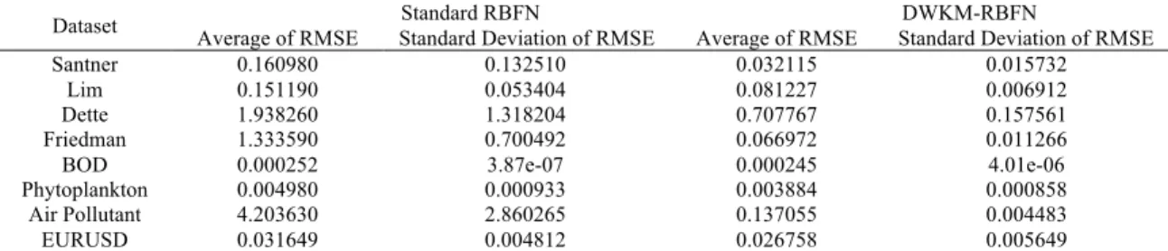
Table 1. Performance of DWKM-RBFN and Standard RBFN prediction results for datasets. Dataset Average of RMSE Standard Deviation of RMSE Standard RBFN Average of RMSE Standard Deviation of RMSE DWKM-RBFN Santner 0.160980 0.132510 0.032115 0.015732
Lim 0.151190 0.053404 0.081227 0.006912 Dette 1.938260 1.318204 0.707767 0.157561 Friedman 1.333590 0.700492 0.066972 0.011266 BOD 0.000252 3.87e-07 0.000245 4.01e-06 Phytoplankton 0.004980 0.000933 0.003884 0.000858 Air Pollutant 4.203630 2.860265 0.137055 0.004483 EURUSD 0.031649 0.004812 0.026758 0.005649
Table 2. Percentage of Improvement for DWKM-RBFN over Standard RBFN by RMSE. Dataset Percentage of Improvement (%)
Santner 80.05
Lim 46.27
Dette 63.48
Friedman 94.98
BOD 2.72
Phytoplankton 22.01 Air Pollutant 96.74
EURUSD 15.45
Results from Table 1 shows that DWKM-RBFN networks outperform standard RBFN in average RMSE and standard deviation of RMSE. All results of average RMSE in Table 1 are calculated using ten times run of each networks. From Table 1, DWKM-RBFN network surpasses the standard RBF in accuracy and network architecture by using training set which consists only 81.8%, 71.8%, 68.5%, and 65.8% of total dataset size for Santner dataset, Lim dataset, Dette dataset, and Friedman dataset, respectively. While DWKM-RBFN network training for real-world dataset involves the BOD dataset, Phytoplankton dataset, Air pollutant dataset and forex EURUSD dataset used only 81.8%, 71.8%, 68.5% and 66.8%, respectively. This means that, it is possible to suitable number of dataset such that, it will provide a network with reduced complexity, faster training time and improved accuracy.
Table 2 shows the results of the percentage of improvement of RMSE for DWKM-RBFN network in compared to standard RBFN. Results showed that DWKM-RBFN network outperform standard RBFN network in term of accuracy more than 80% for Santner dataset, Friedman dataset and air pollutant dataset. Meanwhile, for Lim dataset, Dette dataset, Phytoplankton dataset and forex EURUSD dataset, each obtained improvement in range of 15% to 64%. However, BOD dataset shows no significant improvement for DWKM-RBFN network over standard RBFN with percentage less than 3%. This is due to the high nonlinearity of BOD data, besides, the lack of additional input variable that control the changes in BOD can lead to weakprediction results.
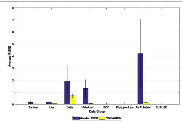
The results from real-world datasets for Phytoplankton dataset and forex EURUSD dataset showed improvement of 22.01% and 15.45%, respectively. Both of this datasets are highly nonlinear data. Possible existence of other environmental factor not included in dataset is the reason behind the low improvement percentage occurs for Phytoplankton dataset. Additionally, for forex EURUSD dataset, the low improvement percentage is due to many possible factors not included in the dataset that also drives the movement of this currency values. Factor that cannot be quantified, such as political influences or natural disaster, can affect the currency fluctuation. Hence, if such factors can quantify and includes in the dataset, improvement in percentage is expected. From Table 1 and Table 2, we observed that DWKM-RBFN network provide such consistent results even that it uses less dataset and still able to perform such satisfying results. The results of prediction from DWKM-RBFN network are consistent as we observed from Table 1, the standard deviation of RMSE was much lower than standard RBFN. Figure 1 shows the error bar plot that displayed the comparison of errors for both the networks. Clearly, the standard RBFN has larger error in compared to DWKM-RBFN network for all datasets.
The DWKM-RBFN network and Standard RBFN performed well in the experiments for dataset with smaller range that lies in [0,1]. However, for larger range of dataset such as air pollutant dataset, the standard RBFN performed poorly in accuracy. Besides, the DWKM-RBFN network is superior in accuracies and the architecture of the network but a proper adjustment in the number of centers for each dataset can enhance the networks accuracy to much higher level. The results in Table 1 shows that even with less dataset used for training, if the right centers are chosen, can impact in prediction accuracy. The uses of huge number of dataset does not always guarantee the desirable prediction accuracies, but sufficient number of dataset that can represent the shape of the distribution for the dataset is enough for providing good prediction results. Furthermore, many of training dataset might contain invalid data that could jeopardize the desired accuracy, not mentioning the size of network it would create and the time taken for training.
Hence, there is no denial on the ability of the DWKM-RBFN network and standard RBFN in prediction, but it comes with a hefty compensation for the accuracy if the proper value of number of centers is not selected. As the number of datasets for the network becomes lesser and it results much simpler network architecture and possibly free of invalid dataset. Although both models provide satisfying results, the network structure and accuracy of the DWKM-RBFN network is superior compared to the standard RBFN network.
Figure 1. Error bar plot for datasets using standard RBFN and DWKM-RBFN. 5. CONCLUSION
Four literatures nonlinear functions and four real-world problems have been simulated in this paper, where we applied for real-world problems on prediction of BOD problem, phytoplankton problem, air pollution problem and forex EURUSD price prediction problem. The performance of both networks has been compared to the case using the Root Mean Squared Error (RMSE) and standard deviation as the criteria for performance measurement and network prediction consistency. Results from all eight studies show that the DWKM-RBFN network is better than the standard RBFN in prediction accuracy and network architecture. Thus, it is possible to improve the accuracy of the proposed network by using statistical methods to choose the best value of number of center to be used for different type of dataset. As conclusion, the proposed network is far superior to the standard RBFN network as for network architecture and accuracy. Since self-organized selection of centers can performed by clustering algorithms for selecting significant centers, sufficient to represent the distribution of dataset for the hidden nodes has been used, it would be interesting if the networks to be tested with high noise training data to verify the efficiency of the chosen clustering algorithm in center selection.
REFERENCES
[1] H. Sarimveis, A. Alexandridis, and G. Bafas, “A fast training algorithm for RBF networks based on subtractive clustering,” Neurocomputing, vol. 51, pp. 501-505, 2003.
[2] A. Alexandridis, E. Chondrodima, N. Giannopoulos, and H. Sarimveis, “A Fast and Efficient Method for Training Categorical Radial Basis Function Networks,” IEEE Trans. Neural Networks Learn. Syst., pp. 1-6, 2016.
[3] A. Alexandridis, E. Chondrodima, N. Giannopoulos, and H. Sarimveis, “A fast and efficient method for training categorical radial basis function networks,” IEEE Trans. Neural Networks Learn. Syst., vol. 28, no. 11, pp. 2831-2836, 2017.
[4] Y. Hu, J. J. You, J. N. K. Liu, and T. He, “An eigenvector based center selection for fast training scheme of RBFNN,” Inf. Sci. (Ny)., vol. 428, pp. 62-75, 2018.
[5] E. M. da Silva, R. D. Maia, and C. D. Cabacinha, “Bee-inspired RBF network for volume estimation of individual trees,” Comput. Electron. Agric., vol. 152, pp. 401-408, 2018.
[6] D. Shan and X. Xu, “Multi-label Learning Model Based on Multi-label Radial Basis Function Neural Network and Regularized Extreme Learning Machine,” Moshi Shibie yu Rengong Zhineng/Pattern Recognit. Artif. Intell., vol. 30, no. 9, 2017.
[7] Y. Sun et al., “The application of RBF neural network based on ant colony clustering algorithm to pressure sensor,” Chinese J. Sensors Actuators, vol. 26, no. 6, 2013.
[9] S. Mirjalili, “Evolutionary Radial Basis Function Networks,” in Studies in Computational Intelligence, 2019, pp. 105-139.
[10] A. Osmanović, S. Halilović, L. A. Ilah, A. Fojnica, and Z. Gromilić, “Machine learning techniques for classification of breast cancer,” in IFMBE Proceedings, 2019.
[11] M. Mohammadi, A. Krishna, S. Nalesh, and S. K. Nandy, “A Hardware Architecture for Radial Basis Function Neural Network Classifier,” IEEE Trans. Parallel Distrib. Syst., 2018.
[12] M. W. L. Moreira, J. J. P. C. Rodrigues, N. Kumar, J. Al-Muhtadi, and V. Korotaev, “Evolutionary radial basis function network for gestational diabetes data analytics,” J. Comput. Sci., 2018.
[13] K. Kavaklioglu, M. F. Koseoglu, and O. Caliskan, “International Journal of Heat and Mass Transfer Experimental investigation and radial basis function network modeling of direct evaporative cooling systems,” Int. J. Heat Mass Transf., vol. 126, pp. 139-150, 2018.
[14] M. Smolik, V. Skala, and Z. Majdisova, “Advances in Engineering Software Vector fi eld radial basis function approximation ☆,” Adv. Eng. Softw., vol. 123, no. 17, pp. 117-129, 2018.
[15] Y. Li, X. Wang, S. Sun, X. Ma, and G. Lu, “Forecasting short-term subway passenger flow under special events scenarios using multiscale radial basis function networks,” Transp. Res. Part C Emerg. Technol., 2017.
[16] G. W. Chang, H. J. Lu, Y. R. Chang, and Y. D. Lee, “An improved neural network-based approach for short-term wind speed and power forecast,” Renew. Energy, 2017.
[17] Q. P. Ha, H. Wahid, H. Duc, and M. Azzi, “Enhanced radial basis function neural networks for ozone level estimation,” Neurocomputing, 2015.
[18] Z. Majdisova and V. Skala, “Radial basis function approximations : comparison and applications,” Appl. Math. Model., vol. 51, pp. 728-743, 2017.
[19] Y. Lei, L. Ding, and W. Zhang, “Generalization Performance of Radial Basis Function Networks,” Neural Networks Learn. Syst. IEEE Trans., vol. 26, no. 3, pp. 551-564, 2015.
[20] C. Arteaga and I. Marrero, “Universal approximation by radial basis function networks of Delsarte translates,” Neural Networks, vol. 46, pp. 299-305, 2013.
[21] S. Lin, “Linear and nonlinear approximation of spherical radial basis function networks ✩,” vol. 35, pp. 86-101, 2016.
[22] M. L. Albalate, “Data reduction techniques in classification processes,” 2007.
[23] S. Haykin, “Neural networks-A comprehensive foundation,” New York: IEEE Press. Herrmann, M., Bauer, H.-U., & Der, R, vol. psychology. pp. pp107-116, 1994.
[24] B. V. Dasarathy, “A computational demand optimization aide for nearest-neighbor-based decision systems,” in Conference Proceedings 1991 IEEE International Conference on Systems, Man, and Cybernetics, 1991, pp. 1777-1782.
[25] B. Dasarathy, “Data mining tasks and methods: Classification: nearest-neighbor approaches,” Handb. data Min. Knowl. Discov., 2002.
[26] J. Jȩdrzejowicz and P. Jȩdrzejowicz, “Distance-based online classifiers,” Expert Syst. Appl., vol. 60, pp. 249-257, 2016.
[27] M. Kirsten and S. Wrobel, “Relational distance-based clustering,” in Proceedings of the 8th international conference on Inductive logic programming, ILP-98, July 22-24, 1998, no. 20237, pp. 261-270.
[28] G. Zhang, C. Zhang, and H. Zhang, “Improved K-means algorithm based on density Canopy,” Knowledge-Based Syst., 2018.
[29] W. L. Zhao, C. H. Deng, and C. W. Ngo, “k-means: A revisit,” Neurocomputing, 2018.
[30] K. Dahiya, “Reducing Neural Network Training Data using Support Vectors,” vol. 0, no. 2, pp. 6-8, 2014.
[31] M. A. Sebtosheikh and A. Salehi, “Lithology prediction by support vector classifiers using inverted seismic attributes data and petrophysical logs as a new approach and investigation of training data set size effect on its performance in a heterogeneous carbonate reservoir,” J. Pet. Sci. Eng., vol. 134, pp. 143-149, 2015.
[32] S. Wang, Z. Li, C. Liu, X. Zhang, and H. Zhang, “Training data reduction to speed up SVM training,” Appl. Intell., vol. 41, no. 2, pp. 405–420, 2014.
[33] S. Mirjalili, “Evolutionary Radial Basis Function Networks,” in Studies in Computational Intelligence, 2019, pp. 105-139.
[34] C. C. Liao, “Genetic k-means algorithm based RBF network for photovoltaic MPP prediction,” Energy, 2010. [35] M. A. Rahman and M. Z. Islam, “A hybrid clustering technique combining a novel genetic algorithm with
K-Means,” Knowledge-Based Syst., 2014.
[36] J. Wu, J. Long, and M. Liu, “Evolving RBF neural networks for rainfall prediction using hybrid particle swarm optimization and genetic algorithm,” Neurocomputing, 2015.
[37] L. Tan, “A clustering K-means algorithm based on improved PSO algorithm,” in Proceedings - 2015 5th International Conference on Communication Systems and Network Technologies, CSNT 2015, 2015.
[38] E. M. da Silva, R. D. Maia, and C. D. Cabacinha, “Bee-inspired RBF network for volume estimation of individual trees,” Comput. Electron. Agric., vol. 152, 2018.
[39] M. Diez, S. Volpi, A. Serani, F. Stern, and E. F. Campana, “Simulation-Based Design Optimization by Sequential Multi-criterion Adaptive Sampling and Dynamic Radial Basis Functions,” in Computational Methods in Applied Sciences, 2019.
[40] H. de Leon-Delgado, R. J. Praga-Alejo, D. S. Gonzalez-Gonzalez, and M. Cantú-Sifuentes, “Multivariate statistical inference in a radial basis function neural network,” Expert Syst. Appl., 2018.
[41] Y. Cui, J. Shi, and Z. Wang, “Lazy Quantum clustering induced radial basis function networks (LQC-RBFN) with effective centers selection and radii determination,” Neurocomputing, 2016.
[42] G. A. Montazer and D. Giveki, “An improved radial basis function neural network for object image retrieval,” Neurocomputing, 2015.
[43] Z. Ramedani, M. Omid, A. Keyhani, S. Shamshirband, and B. Khoshnevisan, “Potential of radial basis function based support vector regression for global solar radiation prediction,” Renew. Sustain. Energy Rev., 2014.
[44] T. Wangchamhan, S. Chiewchanwattana, and K. Sunat, “Efficient algorithms based on the k-means and Chaotic League Championship Algorithm for numeric, categorical, and mixed-type data clustering,” Expert Syst. Appl., 2017.
[45] Q. Que and M. Belkin, “Back to the Future: Radial Basis Function Networks Revisited,” in Proceedings of the 19th International Conference on Artificial Intelligence and Statistics, 2016.
[46] V. K. Chauhan, A. Sharma, and K. Dahiya, “Faster learning by reduction of data access time,” Appl. Intell., 2018. [47] G. Afendras and M. Markatou, “Optimality of training/test size and resampling effectiveness in cross-validation,”
J. Stat. Plan. Inference, vol. 16, no. xxxx, pp. 1-16, 2018.
[48] S. Ougiaroglou, K. I. Diamantaras, and G. Evangelidis, “Exploring the effect of data reduction on Neural Network and Support Vector Machine classification,” Neurocomputing, vol. 280, pp. 101-110, 2017.
[49] M. Bataineh and T. Marler, “Neural network for regression problems with reduced training sets,” Neural Networks, vol. 95, pp. 1–9, 2017.
[50] V. Chouvatut, W. Jindaluang, and E. Boonchieng, “Training set size reduction in large dataset problems,” 2015 Int. Comput. Sci. Eng. Conf., pp. 1-5, 2015.
[51] W. A. Yousef and S. Kundu, “Learning algorithms may perform worse with increasing training set size: Algorithm-data incompatibility,” Comput. Stat. Data Anal., vol. 74, pp. 181-197, 2014.
[52] H. Ismkhan, “I-k-means−+: An iterative clustering algorithm based on an enhanced version of the k-means,” Pattern Recognit., 2018.
[53] S. S. Yu, S. W. Chu, C. M. Wang, Y. K. Chan, and T. C. Chang, “Two improved k-means algorithms,” Appl. Soft Comput. J., 2018.
[54] Z. Kakushadze and W. Yu, “*K-means and cluster models for cancer signatures,” Biomol. Detect. Quantif., 2017. [55] M. Capó, A. Pérez, and J. A. Lozano, “An efficient approximation to the K-means clustering for massive data,”
Knowledge-Based Syst., 2017.
[56] C. Xiong, Z. Hua, K. Lv, and X. Li, “An improved K-means text clustering algorithm by optimizing initial cluster centers,” in Proceedings - 2016 7th International Conference on Cloud Computing and Big Data, CCBD 2016, 2017.
[57] R. Jothi, S. K. Mohanty, and A. Ojha, “DK-means: a deterministic K-means clustering algorithm for gene expression analysis,” Pattern Analysis and Applications, 2017.
[58] S. Maldonado, E. Carrizosa, and R. Weber, “Kernel Penalized K-means: A feature selection method based on Kernel K-means,” Inf. Sci. (Ny)., 2015.
[59] X. Huang, Y. Ye, L. Xiong, R. Y. K. Lau, N. Jiang, and S. Wang, “Time series k-means: A new k-means type smooth subspace clustering for time series data,” Inf. Sci. (Ny)., 2016.
[60] K. M. Kumar and A. R. M. Reddy, “An efficient k-means clustering filtering algorithm using density based initial cluster centers,” Inf. Sci. (Ny)., 2017.
[61] Y. Hanmin, L. Hao, and S. Qianting, “An improved semi-supervised K-means clustering algorithm,” in Proceedings of 2016 IEEE Information Technology, Networking, Electronic and Automation Control Conference, ITNEC 2016, 2016.
[62] Y. Liu, H. P. Yin, and Y. Chai, “An improved kernel k-means clustering algorithm,” in Lecture Notes in Electrical Engineering, 2016.
[63] S. Kant and I. A. Ansari, “An improved K means clustering with Atkinson index to classify liver patient dataset,” Int. J. Syst. Assur. Eng. Manag., 2016.
[64] Y. Ding, Y. Zhao, X. Shen, M. Musuvathi, and T. Mytkowicz, “Yinyang K-means: A drop-in replacement of the classic K-means with consistent speedup,” Icml-2015, 2015.
[65] G. Tzortzis and A. Likas, “The MinMax k-Means clustering algorithm,” in Pattern Recognition, 2014.
[66] I. Melnykov and V. Melnykov, “On K-means algorithm with the use of mahalanobis distances,” Stat. Probab. Lett., 2014.
[67] T. J. Santner, B. J. Williams, and W. I. Notz, The Design and Analysis of Computer Experiments, 1st ed. Springer-Verlag New York, 2003.
[68] Y. B. Lim, J. Sacks, W. J. Studden, and W. J. Welch, “Design and analysis of computer experiments when the output is highly correlated over the input space,” Can. J. Stat., vol. 30, no. 1, pp. 109-126, 2002.
[69] H. Dette and A. Pepelyshev, “Generalized latin hypercube design for computer experiments,” Technometrics, vol. 52, no. 4, pp. 421-429, 2010.
[70] J. H. Friedman, M. Adaptive, and R. Splines, “Multivariate Adaptive Regression Splines,” Ann. Stat., vol. 19, no. 1, pp. 1-67, 1991.
[71] L. E. Aik and Z. Zainuddin, “An Improved Fast Training Algorithm for RBF Networks Using Symmetry-Based Fuzzy C-Means Clustering Overview of Fuzzy C-Means Clustering Method,” MATEMATIKA, vol. 24, no. 2, pp. 141-148, 2008.