Parameter Estimation of Vehicle Handling Model Using Genetic Algorithm

Parameter Estimation of Vehicle

Handling Model Using Genetic Algorithm

and S. Azadi 1

This paper implements a derivative free optimization method called `Genetic Algorithm' to estimate the parameters of a four-wheel, three degrees of freedom vehicle handling model. At rst the model is developed containing a non-linear tire model called `Fiala'. Then, an error function is dened and the `Genetic Algorithm' optimization method is introduced and applied to minimize the error. Finally, verication of parameter estimation is checked.

INTRODUCTION

In order to design a more ecient vehicle, extensive simulations must be performed and vehicle responses should be analyzed, therefore, mathematical vehicle models for lateral and longitudinal dynamics, struc-ture, NVH and etc. are needed. However, as each model consists of several parameters, this more com-plex model requires more parameters to be run.

Some of the parameters are known or easily measurable. For example, geometrical properties, such as tread width and wheelbase, are known. However, there are some parameters that are unknown and directly immeasurable, such as tire model parameters, sprung and unsprung mass, suspension stiness and etc. These parameters are usually estimated through an identication process and vehicle testing. This means that parameter identication plays an important role in vehicle simulations. This paper deals with the lateral dynamics of a passenger car and focuses on identifying the parameters of a vehicle handling model. A review of the literature shows numerous meth-ods of parameter estimation. Bolzen et al. have estimated the magic formula tire model parameters of a 2DOF vehicle model, using an extended Kalman Filter 1]. Hauqe and Schuller implemented the special case of a neural network, called the Fourier series neural network, to identify vehicle model parameters 2].

*. Corresponding Author, Department of Mechanical Engi-neering, Sharif University of Technology, Tehran, I.R. Iran.

1. Department of Mechanical Engineering, Khajeh-Nassir Toosi University of Technology, Tehran, I.R. Iran.

Wohler et al. have identied the cornering stiness of a tire model in a 2DOF vehicle model, as a function of the slip angle, using the evolution method and the mode-ltering method 3]. Also, Huang et al., by using random steer as an input of the model, have estimated some parameters of the 2DOF and 3DOF vehicle model in the frequency domain 4].

The identication method in this paper is based on minimizing the error between model and reference outputs, which is developed by simulation of a complex vehicle model (a model with more than 100 DOFs) in ADAMS, a validated software in vehicle dynamics.

The present paper aims to set up a procedure that will make it possible to use road test data to obtain unknown parameters.

In this paper, a quadricycle 3DOF vehicle model is developed accounting for lateral velocity, yaw rate and roll angle as degrees of freedom. Then, the `Genetic Algorithm' optimizing method is applied using reference data and the unknown parameters are estimated. Finally, validation of the process is checked using another data set, which will be explained later.

VEHICLE MODEL FORMULATION FOR

PARAMETERS IDENTIFICATION

For simulating the lateral dynamics of the vehicle, a 4-wheel 3DOF model is used containing lateral velocity (V), yaw rate (r) and roll angle (). The input of the

model is the steering angle () on the front tires. Also,

the continuum mass of the vehicle is modeled by three lumped masses, which are front and rear unsprung masses (M

uf M

ur) and sprung mass ( M

vehicle mass is: M t= M s+ M uf+ M ur : (1)

In order to derive the equation of motion, a moving reference frame is attached to the vehicle with its origin at the center of gravity, as shown in Figure 1.

Since the coordinate system is attached to the vehicle, the inertia properties of the vehicle will remain constant. Also, as the result of symmetry assumption, all the products of inertia are ignored. The state variables are assumed to be lateral velocity, yaw rate and roll angle.

Using the above assumptions, the equations de-scribing the motion are 5,6]:

M t( _

V+ru)+M s h s =F yfr+ F yfl+ F yrr+ F yfl (2) I xx +M s h

s( _

V +ru) =L s

(3)

I zz_

r=a(F yfr+

F yfl)

;b(F yrr+ F yrl) (4) where: L s= M s gh s ;K ;C _ (5) where M

s is the sprung mass, which is the mass

sup-ported by the vehicle suspension,I

xxis the sprung mass

moment of inertia about longitudinal axis (x),I

zzis the

moment of inertia of the entire vehicle about vertical axis (z),K

and C

are roll stiness and roll damping

coecient of suspensions, respectively,h

sis the vertical

distance of CG from the roll axis , a and b are the

distances of the front and rear axles from CG, u is

the longitudinal speed of the vehicle, which is constant in vehicle maneuvers, andF

yfr F yfl F yrr F

yrlare the

tire cornering forces of front right, front left, rear right and rear left, respectively.

The cornering force of a tire is mainly dependent on the slip angle, vertical load, longitudinal slip and camber angle of that tire. In this paper a tire model called `Fiala' 7], in which the cornering force of the tire is a function of the cornering stiness, vertical load, slip

Figure1. Vehicle coordinate system.

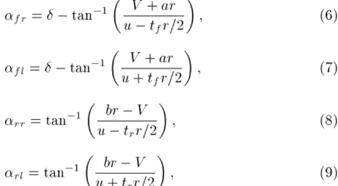
angle and longitudinal slip has been used and the eects of camber angle and aligning moments are ignored. In order to compute tire forces, the slip angles of the tire should be calculated as below 6]:

fr=

;tan ;1

V +ar u;t

f r=2 (6) fl= ;tan ;1

V +ar u+t

f r=2

(7)

rr= tan ;1

br;V u;t

r r=2

(8)

rl= tan ;1

br;V u+t

r r=2

(9)

whereis the steer angle as the input of the model and t

f t

rare the front and rear tread widths of the vehicle,

respectively.

Also, for obtaining the lateral load transfer, some equations to describe vertical forces on each tire have been written. In this paper, lateral load transfer is assumed to be the result of three phenomena, which are body roll, roll center height and unsprung mass 6]. Lateral load transfer, due to body roll, is as follows:

F f1=

k f h s M s K t f

:(a ycos

+gsin) (10) F

r1= k r h s M s K t r

:(a ycos

+gsin) (11)

wherek fand

k

rare the front and rear roll stiness and a

y is the lateral acceleration, which is: a

y= _

V +ru+ M s h s M t : (12)

Lateral load transfer, due to roll center height, is as follows:

F f2=

M s bh f a y t f( a+b)

(13)

F r2=

M s ah r a y t r( a+b)

(14)

where h f and

h

r are the front and rear roll center

heights, respectively.

And lateral load transfer, due to unsprung masses, is:

F f3=

M uf a y h f t f (15) F r3=

M ur a y h r t r : (16)

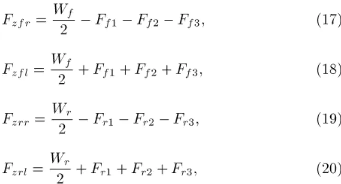
The vertical load on each tire can be described by the following equations: F zfr= W f

2 ;F f1 ;F f2 ;F f3 (17) F zfl= W f

2 +F f1+

F f2+

F f3 (18) F zrr= W r

2 ;F r1 ;F r2 ;F r3 (19) F zrl= W r

2 +F r1+

F r2+

F r3 (20) where W f and W

r are the static load distribution on

the front and rear axles and can be computed by the following equations: W f = M t g b a+b

(21) W r= M t g a a+b

: (22)

TIRE MODEL

As mentioned before in this paper, a tire model called `Fiala' is used in the vehicle dynamic simulation. This model calculates tire cornering forces as a function of vertical load (F

z), slip angle (

), cornering stiness

(C

), longitudinal slip ( S

s) and the maximum and

minimum friction coecients (UmaxUmin) between tire

contact patch and road 7]. The relations of this model, which nally return the tire cornering force, are:

U =Umax;(Umax;Umin):S s (23) F y= ( UjF z

jsgn() > cri

UjF

z

j:(1;H3):sgn() cri (24) where: S s= q S2

s+ tan

2 ₍₂₅₎

cri= tan ;1

3UjF z j C (26)

H = 1; C

jtanj

3Uj F z

j

: (27)

ESTIMATION OF VEHICLE PARAMETERS

The unknown parameters, which are to be identied, are front and rear tire cornering stiness, entire vehicle yaw moment of inertia, sprung mass roll moment of inertia, roll stiness and roll damping coecients. The

unknown vector, (), is the set of under-estimating

parameters and can be written as:

= C f C r I zz I xx K C ] : (28)

Since the model is a 3DOF and contains three equa-tions of motion in terms of unknown parameters, the equations can be described as:

f() = 0 (29)

where `f' is a 31 vector containing Equations 2 to 4

and may be a nonlinear relation in . Note that in

the identication process, the state variables are known and Equation 29 is an algebraic equation in terms of

and not a dierential equation.

The main idea in identication is to nd an approximate solution,

l, which minimizes the error as

dened below:

e() =

3 X i=1 (w i f i)

2 (30)

where f

i is the

ith row of vector `f 0 and

w i is the

suitable weighting factor used in order to have the same order in f

i.

For minimizing the error, the `Genetic Algorithm' optimizing method is applied to the problem.

Except for the unknown parameters, the others used in the identication process are listed in Table 1.

GENETIC ALGORITHM METHOD

The Genetic Algorithm method (GA) 8,9] is a stochas-tic optimization method which is based on the concepts of natural selection and evolution processes. Since this method, like the other random based search methods, does not require the derivation of objective function, they are also called `Derivative-Free' methods.

Table 1. The known vehicle parameters. a= 0:873 (m) M

s= 716 (kg) b= 1:497 (m) M

uf = 64 (kg) t

f = 1

:404 (m) M

ur= 60 (kg) t

r= 1

:384 (m) u= 50 (km/hr) h

s= 0

:3972 (m) h

f = 0

:160 (m) h r= 0

:105 (m)

Tire Model Parameters

s= 0 :05

GA was rst proposed and investigated by John Holland at the University of Michigan 10] and which, as a maximizing method, has since received increasing amounts of attention, due to its versatile optimization capabilities for both continuous and discrete problems. Since GA is derivative-free, it can be used for problems with very complex objective functions such as structure and parameter identication. Also, as a result of its randomness nature, GA is a global optimizer and is able to nd the global optimum, given enough computation time.

In order to use the GA method, each of the parameters should be encoded into a binary string called a `Gene'. The genes will then, combine with each other resulting in a `Chromosome' and a non-negative real value called `Fitness' is assigned to each chromosome. The goal of GA is to maximize the tness value, therefore, in minimizing problems, `Fitness' should be dened in such a manner that maximizing the tness value results in minimizing the objective function.

In the GA method, a population of chromosomes is randomly generated and then evolved repeatedly towards a better overall tness value. In each gen-eration, the GA constructs a new population using genetic operators such as `Crossover' and `Mutation', remembering that members with higher tness values are more likely to take part in mating operations.

The algorithm of running this method can be summarized as:

- Encoding the parameters into a binary string, - Fitness evaluation,

- Parents' selection, - Crossover operation, - Mutation operation.

In this paper, the vector is encoded into the

binary string with a 39 bits length for the 6 parameters of . The bits 1 to 7 and 8 to 14 are denoted to C

f C

r, respectively. Also the bits 15 to 20 for I

zz,

21 to 25 forI

xx, 26 to 32 for K

and 33 to 39 for C

are assigned. Also, the tness function in this paper is dened as:

Fitness () = A e()

(31)

whereAis a positive constant used for dening tness

function as a maximizing problem.

After the tness evaluation of all chromosomes is completed, the selection operation determines which parents will take part in mating in order to produce ospring for the next generation. In this paper, the parents are chosen with a selection probability

proportional to their tness values. The selection probability of each parent can be dened as:

p

i= (Fitness) i n

P k=1

(Fitness)k

(32)

wherenis the number of chromosomes in a generation.

After parent selection, the crossover operation is applied to the selected pair of parents with a prob-ability called `Crossover Rate'. In this paper, `One-Point Crossover', which is the most common and basic crossover operator, is used. In this method a crossover point on the selected chromosomes is randomly found and two parents' chromosomes are interchanged at this point.

When the crossover operation is completed, the mutation operator, which is ipping a bit, is applied to the selected chromosome with a very low probability called `Mutation Rate'. Mutation can prevent the population from stagnating at local optima. Usually, the crossover rate is above 0.8 and the mutation rate is below 0.05 and, if the mutation rate is high (above 0.1), the GA will approach to a simple and primitive random search.

The above phases of GA will be repeated until the terminating criterion is satised. In this paper, the terminating criterion is assumed as: When the average of the tness values of a generation is not less than 98% of the maximum tness, the process will stop.

RESULTS OF IDENTIFICATION

To apply the GA optimization method, a computer code has been written in MATLAB software and then the GA has been applied to minimize the error and the unknown vector,, has been obtained.

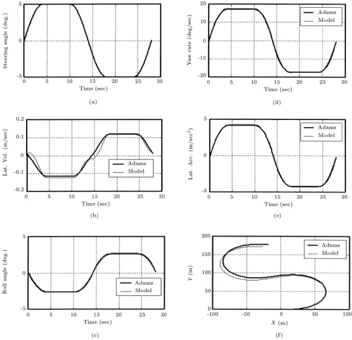
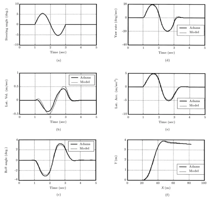
For identication, a combined sinusoidal and step steering angle, as an input of the model, is used, in order to obtain both the transient and steady state responses of the vehicle. This steering signal is shown in Figure 2a.

As mentioned before, the reference data for iden-tication has been obtained by ADAMS. After the process has converged to the solution and the unknown vector,, has been estimated, the model is solved using

land the results are compared with the reference data,

as illustrated in Figures 2b to 2f. The path of the vehicle is identied and the Adams model is plotted during the simulation in Figure 2f.

Also, the convergence of the identication process is illustrated in Figure 3. As seen, the average of the tness values of the generation increases during the process.

In general, the identication process is always followed by a validation process using another data set.

Figure2. (a) is the input steering for identication and (b) to (f) are the results of identication.

Figure3. Convergence of GA method used for

identication.

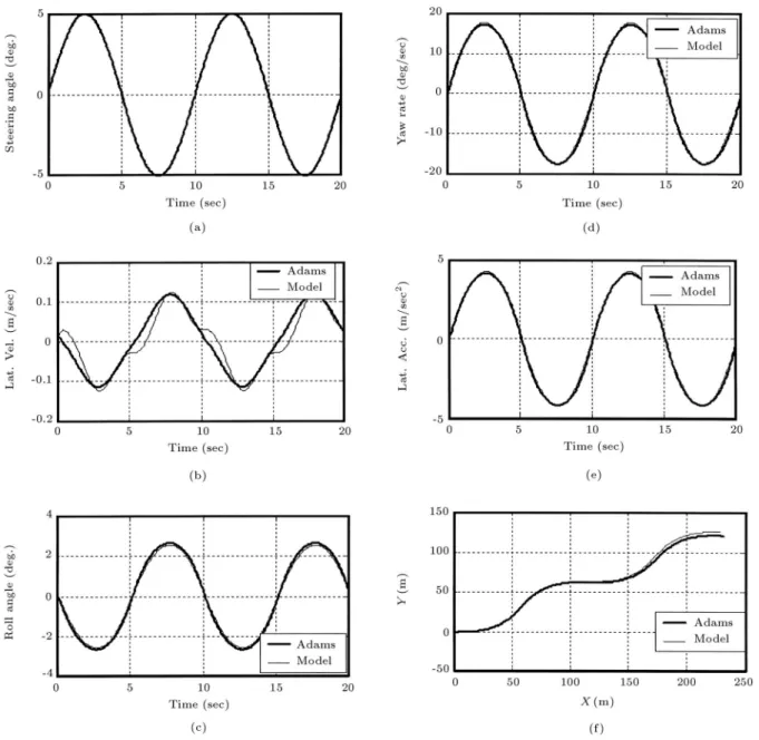
For validation, a sinusoidal input steering angle, which is a slalom test (the vehicle moves sinusoidal) input, with frequency 0.1 Hz, is used, as shown in Figure 4a. The result of the validation process is illustrated in Figures 4b to 4f. Note that the vehicle has the same forward velocity, 50 (km/hr).

The estimated vector, l, is:

l= 20588

21193946276300002505]:

Another validation check is performed, using a single lane change maneuver at 60 (km/hr) forward velocity. The steer angle of this maneuver, which is a sharp and quick sinusoidal signal, is shown in Figure 5a. The outputs of identied and Adams models are compared with each other and shown in Figures 5b to 5f.

Figure 4. (a) is the input steering for the rst validation process and (b) to (f) are the results of this validation.

Similar to the combined input used for identica-tion, in the validation phase, the same variables (lateral velocity, roll angle, yaw rate, lateral acceleration and path followed by the vehicle) are shown.

The lateral velocity is very sensitive to the non-linear behavior of the suspension components and tire. Since in the 3DOF model all the suspension non-linear dynamics are ignored, the lateral velocity of the identied model has more error, compared with the reference data, than the roll angle and yaw rate.

CONCLUSIONS

In this paper, it is illustrated that some of the vehicle model parameters, which are directly immeasurable, can be estimated using one of the optimization

meth-ods. The data used for identication was obtained by simulating a complex model in Adams, however, this method can be implemented using road test data to get the value of the parameters for a real vehi-cle.

Also, it is illustrated that, for identication of a continuous system, such as a vehicle handling model, the optimization techniques (like the GA method) can be used instead of discretizing the model of the system and using the conventional methods of identication.

ACKNOWLEDGMENT

The authors thank the AIRIC (Automotive Industries Research and Innovation Center) for their permission to use Adams software and its related data.

Figure 5. (a) is the input steering for the second validation process and (b) to (f) are the results of this validation.

REFERENCES

1. Bolzern, P., Cheli, F., Falciola, G. and Resta, F. \Estimation of the non-linear suspension tyre corner-ing forces from experimental road test data", Vehicle System Dynamics,31(1), pp 23-34 (1999).

2. Haque, I. and Schuller, J. \Fourier series-based neural network for vehicle system identication",Innovation in Vehicle Design and Development, 101, pp 35-43

(1999).

3. Wohler, A., Jurgensohn, T. and Willumeit, H.P. \Iden-tication of system parameters of simulation models for driving control systems", SAE Paper no. 945070

(1994).

4. Huang, F., Chen, J.R. and Tsai, L.W. \The use of ran-dom steer test data for vehicle parameter estimation", SAE Paper no. 930830 (1993).

5. Gillespie, T.D., Fundamental of Vehicle Dynamics, Warrendale, PA, Society of Automotive Engineering, Inc. (1992).

6. Will, A.B. and Zak, S.H. \Modelling and control of an automated vehicle",Vehicle System Dynamics,27(3),

pp 131-155 (1997).

7. Using Adams/Tire, Mechanical Dynamics Incorpora-tion(2000).

8. Goldberg, D.E., Genetic Algorithms in Search, Opti-mization and Machine Learning, New York, Addison-Wesley (1989).

9. Jang, J.S.R. and Sun, C.T. and Mizutani, E., Neuro-Fuzzy and Soft Computing, Prentice Hall (1997). 10. Holland, J.,Adaptation in Natural and Articial

Sys-tems, Ann Arbor, The University of Michigan Press (1975).