Numerical Modeling of Hydraulic Fracturing in Oil Sands

Numerical Modeling of Hydraulic

Fracturing in Oil Sands

A. Pak

_{and D.H. Chan}

Hydraulic fracturing is a widely used and ecient technique for enhancing oil extraction from heavy oil sands deposits. Application of this technique has been extended from cemented rocks to uncemented materials, such as oil sands. Models, which have originally been developed for analyzing hydraulic fracturing in rocks, are in general not satisfactory for oil sands. This is due to a high leak-o in oil sands, which causes the mechanism of hydraulic fracturing to be dierent from that for rocks. A thermal hydro-mechanical fracture nite element model is developed, which is able to simulate hydraulic fracturing under isothermal and non-isothermal conditions. Plane strain or axisymmetric hydraulic fracture problems can be simulated by this model and various boundary conditions, such as specied pore pressure/uid ux, specied temperature/heat ux, and specied loads/traction, can be modeled. The developed model has been veried by comparing its results to existing analytical and numerical solutions for thermo-elastic consolidation problems. The model has been used to simulate a laboratory experiment of hydraulic fracture propagation in oil sands. The results from the numerical model are in agreement with experimental observations. The numerical model and laboratory experiments both indicate that, for uncemented porous materials, such as sands (as opposed to rocks), a single planar fracture is unlikely to occur and a system of multiple fractures or a fracture zone consisting of interconnected tiny cracks should be expected.

INTRODUCTION

Hydraulic fracturing is a widely used technique to enhance oil and gas production. The technique was introduced to the petroleum industry in 1947, and is now a standard operating procedure. By 1981, more than 800,000 hydro fracturing treatments had been performed and recorded. Today, about 35% to 40% of all currently drilled wells are hydraulically fractured [1]. Since its inception, hydraulic fracturing has devel-oped from a simple low volume and low injection rate reservoir stimulation technique to a highly engineered and complex procedure that can be used for many pur-poses. Figure 1 depicts a typical hydraulic fracturing process in the petroleum industry. The procedure is as follows. First, a neat uid, such as water (called

1. Department of Civil Engineering, Sharif University of Technology, Tehran, Iran.

2. Department of Civil and Environmental Engineering, University of Alberta, 3-133 NREF Building, T6G 2W2, Edmonton, Al1berta, Canada.

*. To whom correspondence should be addressed. E-mail: pak@sharif.edu.

Figure 1. Typical hydraulic fracturing treatment in petroleum industry (after [1]).

`pad'), is pumped into the well at the desired depth (pay zone), to initiate the fracture and to establish its propagation. This is followed by pumping slurry, which is a uid mixed with a propping agent, such as sand (often called a `proppant'). This slurry continues to extend the fracture and concurrently carries the proppant deeply into the fracture. After pumping, the injected uid chemically breaks down to a lower viscosity and ows back out of the well, leaving a highly conductive propped fracture for oil and/or gas to easily

ow from the extremities of the formation into the well. It is generally assumed that the induced fracture has two wings, which extend in opposite directions from the well and is oriented, more or less, in a vertical plane. Other fracture congurations, such as horizontal fractures, are also reported to occur, but they constitute a relatively low percentage of situations documented. Experience indicates that at a depth of below 600 meters, fractures are usually oriented vertically. At shallow depths, horizontal fractures have been reported [1]. The fracture pattern, however, may not be the same for dierent types of soil and rock.

`Oil sands' exist in some parts of the world as thick deposits in deep and semi-deep underground layers. For extraction of oil from oil sand deposits, one of the widely used methods, as described above, is hydrofracturing, in which hot water/steam is injected into the wells at a very high rate and temperature. Although sand is a cohesionless material, the viscous bitumen that exists in the porous medium causes the combination of sand and bitumen to behave like a porous rock that may experience fracturing due to high injection pressure. The study of types and patterns of fracture in uncemented oil sand deposits, by means of numerical modeling, is the basic objective of this paper. For decades, petroleum engineers have been de-veloping models for simulating hydraulic fracturing in oil reservoirs. In the early 1960's, the industry felt the need for a design tool for this fast growing technique. In response to this need, a number of two-dimensional (2-D) models were developed for designing hydraulic fracturing treatments. This type of simple closed form solution has been used by the industry with some success; however, as the technology progressed from low volume/rate to high volume/rate treatments in more sophisticated and massive hydraulic fracturing projects, the industry demanded more rigorous design methods in order to minimize costs. In the last 20 years, a number of 2-D and 3-D numerical models have been developed (some of these models will be discussed later). The most common equations used in these numerical models are uid ow and heat transfer equations, which are usually solved iteratively. Geomechanical aspects are incorporated in some of the models, mostly in an uncoupled manner. Mainly vertical or horizontal planar fractures were considered, based on the 2-D closed form solutions mentioned above. The degree of sophistication of these models varies considerably and their results cannot be vali-dated with much condence. The main problem in validating these models is that the conguration of the induced fracture is not really known; therefore, the results of the model are usually evaluated based on uid injection pressure measurements and/or the production history of the well.

The application of these models to oil sands,

however, has not been very successful and predictions of the model, in some cases, have been poor. Some researchers attribute the discrepancy to the eect of high leak-o rates in oil sands. On the other hand, the peculiar characteristics of oil sand, such as an inter-locked structure with a high dilation rate, a nonlinear stress-strain behavior with strain softening after the peak, a dilation phenomenon at shear failure and a temperature-dependent behavior, may also contribute to the discrepancy between model predictions and eld measurements.

In this paper, a brief overview of the earlier stud-ies will be presented and a mathematical formulation of the developed fully coupled thermal hydro-mechanical fracture model will be discussed in detail. Modeling of the fracture process and its numerical treatment will then be explained and benchmarking of the developed nite element model will be presented by comparing its results to the existing analytical, numerical and experimental solutions.

EARLIER STUDIES OF HYDRAULIC FRACTURING

Zheltov and Khristianovitch [2], Perkins and Kern [3] and Geertsma and Deklerk [4] are among the rst investigators to develop models for hydraulic frac-turing. Zheltov and Khristianovitch [2] introduced the concept of mobile equilibrium, i.e. slow moving fracture propagation as a result of hydraulic action. Geertsma and Deklerk [4] used their concepts and provided a closed form solution for a planar fracture. This model is based on the assumption of plane strain deformation in a `horizontal plane' and is usually called the GdK model. Perkins and Kern [3] proposed a dierent closed form solution for hydraulic fracture propagation problems. The model is based on the assumption of plane strain deformation in a `vertical plane'. Nordgren [5] improved this work by incorpo-rating the eect of leak-o and, hence, this model is usually called PKN. In these models, the height of the fracture, hf, is considered to be known, which is

equal to the thickness of the oil-bearing layer (pay). For the determination of other values, such as fracture length (Lf), maximum fracture opening and injection

pressure, a set of equations has been derived.

There have been some eorts to simulate 3-D frac-ture propagation [6,7]. In these models, the assumption of isotropic elasticity is used and the eects of pore pressure are neglected. The elasticity equations are coupled with the equation of ow inside the fractures. In these models, the concept of inducing a planar fracture is retained but the height of the fracture is not xed and varies with changes in stress. Fracture extension is controlled by a linear elastic fracture mechanics criterion. Advani et al. [8] developed a nite

element program for modeling 3-D hydraulic fractures in multi-layered reservoirs. They extended the earlier work of the Pseudo three-dimensional (P3D) model presented by Advani and Lee [9] and other investigators in the early 80's. This work investigated tensile planar hydraulic fracture propagation in layered reservoirs with elastic behavior.

Settari and Raisbeck [10,11] provided two of the early work on hydraulic fracture simulation in `oil sand deposits'. In 1979, they developed a two dimensional nite dierence model for single-phase compressible uid ow in a linear elastic porous material with a tensile fracture, similar to the PKN model. This model was extended to a two-phase thermal ow [11] in order to describe the process of a rst cycle steam injection for three dierent fracture geometries.

Atukorala [12] developed a nite element model for simulating either horizontal or vertical hydraulic fracturing in oil sands. In this work, for the sake of simplicity, the uid ow analysis was separated from stress analysis. These two equations were solved iteratively by imposing a compatibility condition on the volume of the uid in the fracture. The fracture shape was assumed elliptic with blunt tips, in order to avoid the singularity of stresses at the crack tip. A linear elastic fracture mechanics criterion was used for analyzing the tensile fracture in a nonlinear elastic domain. No thermal eect was considered in this study. Settari et al. [13] investigated the eects of soil deformation and fracture on the reservoir in a partially coupled manner. The eect of leak-o on fracture dimensions was emphasized. Oil sand failure was considered to be shear failure with a Mohr-Coulomb criterion. Dilation was not modeled in this work, but it was assumed that a constant change in volumetric strain occurs after reaching a peak shear stress (fail-ure). They developed a computer program, called CONS, based on the above, partially coupled stress-ow, analysis. Settari [14,15] extended this work by incorporating temperature eects (thermal ow) in the formulation.

Frydman and Fontoura [16] simulated the process of borehole pressurization, the mechanism for which is the same as hydraulic fracture treatment with a coupled hydromechanical approach. They developed a new fracture element, considering the eect of a cohesive zone in crack analysis. In their work, the direction of the fracture propagation was predened and no thermal eect was considered.

Ouyang et al. [17] developed a mathematical model and employed an adaptive nite element scheme to simulate the distribution of proppant in a propagat-ing hydraulic fracture.

Itaoka et al. [18] studied the crack growth behav-ior under high tectonic stress, conditions corresponding to great depths. Their study presents a nite element

model for the analysis of hydraulic fracturing, taking into account the mixed-mode fracture. They inves-tigated crack growth behavior as the mode of crack propagation.

Yang et al. [19] numerically studied the eect of heterogeneity and permeability on the initiation and propagation of hydraulic fracturing.

Reynolds et al. [20] used Stimplan software pack-age to determine the optimum fracture dimensions, sizing and sand schedule. Stimplan is a pseudo 3-D, nu-merical model performing an implicit nite dierence solution to basic equations of mass balance, elasticity and uid ow.

Lu et al. [21] developed a pseudo 3-D hydraulic fracturing using radial ow, which made a better prediction regarding fracture height.

Cook et al. [22] conducted a joint experimental-numerical study regarding the exploration of near-well bore mechanics. An experimental procedure, using a true-triaxial apparatus, was developed for the laboratory simulation of slurry injection, and a Discrete Element Method (DEM) numerical model was used for simulation of the experiments. They found that, under isotropic horizontal stress conditions, multiple vertical fractures were induced and propagated in random orientations.

In the early models, it was assumed that fracture in oil sand is similar to fracture in soft cemented rock, such as sandstone; however, the prediction of these models did not match eld observations. For example, the fracture length was smaller than the value predicted by the models, the fracture opening was larger and the injectivity was much higher than anticipated. These facts indicated that hydraulic fracturing in oil sand, contrary to rock, is dominated by leak-o. This high leak-o cannot be adequately described by classical models, such as those proposed by Carter [23] or Nordgren [5]. In order to describe this situation, geomechanical aspects have to be invoked. By incorporating the geomechanical behavior of oil sand in the model, such as shear failure and dilation eects (and the corresponding increase in porosity and permeability), a signicant improvement in the results of the model was observed. From a reservoir engineering viewpoint, the main objective of modeling is being able to predict the production rates of oil wells. Thus, geomechanical aspects are employed in these models, mainly to better improve their prediction ability.

Fracture modeling in porous materials is clearly dependent on the stress eld in the soil, as well as pore uid pressures. Therefore, contrary to most available reservoir engineering models, any attempt to simulate hydraulic fracturing in oil sand deposits should incor-porate a detailed stress/deformation analysis.

four processes are acting simultaneously. Ground deformation, uid ow, heat transfer, and fracturing phenomenon are the main issues involved in hydraulic fracturing. Therefore, for the modeling of hydraulic fracturing in geomaterials, at least three conservation laws for applied load, uid ow, and heat transfer, in the form of three partial dierential equations, have to be solved simultaneously. Fracture conguration should be based on stress/deformation analysis in the ground. In this case, imposing a kind of prescribed fracture geometry on the model is not necessary. FORMULATION OF THE FULLY

COUPLED THERMAL

HYDROMECHANICAL (THM) MODEL In formulating the model, three partial dierential equations of equilibrium, continuity of uid ow, and heat transfer are considered in incremental forms. Changes in displacement in three directions, fUg, changes in pore pressure P , and changes in tem-perature T , are the primary unknowns, which dene the state of any point inside the domain. Since small strains/displacements are assumed, fUg, P and T , during a time increment, `t', are small and sec-ond (or higher) order incremental terms are neglected in the formulation. In this section, a superimposed dot means a derivative with respect to time, `*' stands for nodal values and `-' means prescribed values. Subscript `t' means the value at time t, and subscript `,' indicates a derivative with respect to the coordinate axes.

An equilibrium equation is used as the basis for the deformation analysis. The equilibrium equation in an incremental form reads as follows [24,25]:

ij;j+ Fi= m0 Ui+ C0 _Ui: (1)

A weighted residual method is used for obtaining the weak form of Equation 1. After integration by parts:

Z

S

ijnj!ds

Z

V

ij!;jdV

= Z

V

( Fi+ m0Ui+ c0Ui)!dV;

(2) the following boundary conditions are considered (Fig-ure 2):

- Stress boundary condition (natural B.C.):

ijnj= tsi on S; (3)

- geometric boundary condition (essential B.C.):

Ui= Ui on Su: (4)

Figure 2. Boundary conditions of a typical domain.

Since dynamic eects are not considered in this study, inertia and damping terms will be neglected. The prin-ciple of eective stress can be written in an expanded form incorporating the eect of thermal expansion:

ij = ij0 P ij

= Dijkl

"kl 1₃sklT

P ij: (5)

For consistency with the other two conservation laws, `P ' is considered to be positive in compression. Soil/rock particles are considered to be incompress-ible and the eect of creep and/or other strains are disregarded in Equation 5. Assumption of the in-compressibility of solid grains is usually valid, since the compressibility of pore uid, especially pore uid with occluded gas bubbles, such as oil (bitumen), is very high. Thus, in comparison, the compressibility of solid grains can be neglected. Equation 5 can be used for substituting total stress with eective stress in Equation 2.

In order to obtain the nite element form of Equation 2, spatial discretization can be performed, using the following relationships:

Ui= [N]fUg; "ij= [B]fUg;

"V = [C]fUg;

P =< NP > fPg; P;j = [BP]fPg;

T =< NT > fTg; T;j = [BT]fTg: (6)

By employing the Galerkin method:

[!] = [N] and [!];j = [B]; (7)

`N' indicates the shape function matrix and `B' is the derivative of shape functions, with respect to the spatial coordinates x, y and z. In order to make it possible to use dierent interpolation schemes for calculating displacements, pore uid pressures, and temperatures, dierent `N' and `B' will be used for

pore uid pressures and temperatures. These will be designated by subscripts `P ' and `T ', respectively. For calculating displacements, 8-node rectangular isopara-metric elements are used. For calculating pore pres-sures and temperatures, however, 8-node rectangular elements are changed to 4-node rectangular elements by using the appropriate shape functions. It has been generally observed [26,27] that, in order to obtain com-patible coupled elds, the displacement interpolation should be one order higher than the pore pressure interpolation. Also, Aboustit et al. [28] have reported that the use of a 4-node rectangular element for pore pressures, along with an 8-node rectangular element for displacements, resulted in less oscillation in the analysis of a consolidation problem (compared to a case in which an 8-node element was used for both pore pressure and displacements).

By substituting Equations 3 to 7 into Equation 2, the following equation is obtained:

0

@ Z

V

[B]T_[D][B]dV

1 A fU_g

+ 0 @Z

V

[B]T_{fmg < N} P > dV

1 A fP_g

+ 0 @Z

V

[B]T_[D]1

3Sfmg < NT > dV 1 A fT_g

= Z

S

[N]T_ft SgdS +

Z

lim itsV[N]T( fF g

+ m0_{f Ug + c}0_{f _Ug)dV: (8)}

In Equation 8, fmg represents the Kronecker delta in vector form. The nal nite element form of this equation would be:

[K11]U+ [K12]P+ [K13]T= fF1g; (9)

where K11, K12 and K13represent the factors of U,

P _{and T in Equation 8, respectively, and the}

whole right-hand side of this equation is shown as F1.

For uid ow, the mass continuity equation for porous media is used [29]:

r:(v) G = _@t@ (): (10)

By applying the weighted residual method to obtain the weak form of this equation and then integrating by

parts, Equation 10 becomes: Z

S

(v)ini!dS

Z

V

(v)i!;idV =

Z

V

@

@t()!dV +

Z

V

G!dV: (11)

Two types of boundary condition are considered as follows (shown in Figure 2):

- Specied velocity (ux) at the boundary:

vi= vi on Sv; (12)

- Specied pore uid pressure at the boundary:

P = P on Sp: (13)

The terms , , @_@t, @_@t and vi can be substituted with

relations described below, assuming that the rate of change, with respect to time, can be approximated by the change during the time increment t:

a) Porosity t=

VV

Vb

t=

Vb VS

Vb ; (14)

where Vb is the bulk volume of soil/rock and VV

and Vs are the volume of voids and the volume of

solids, respectively.

t+t= (Vb+ V_(Vb) (Vs+ Vs)

b+ Vb) : (15)

Now, Vb = "V:Vb by denition and Vs =

VsST , assuming that the change in the volume

of solids can be mainly attributed to the thermal expansion of solids, because the compressibility of solids compared to the compressibility of pore uid and bulk medium, is negligible. Hence, the volume change of solids, due to change in pore pressure and eective stresses, can be ignored. Therefore, by substitution for Vb and Vs in Equation 15

and some manipulations, one obtains: t+t= _{1 + "}1

V [t+ "V St(1 t)]; (16)

and:

= t+t t=_{1 + "}1 t

V("V St); (17)

b) Fluid density: Variations of uid density with changes in pressure and temperature can be de-scribed as follows:

Assuming that P and T are the coecients of

uid thermal expansion and uid compressibility, respectively, Equation 18 can be written for time `t + t' in the following form:

t+t= t(1 + TP )(1 PT ); (19)

= t+t t= tTP tPT

tTPP T t(TP PT ); (20)

c) Fluid velocity: Darcy's law, in general index form, is given by:

vi= Kij_@x@H

j; (21)

where K is permeability (m/sec) and H is total head. Representing K in terms of absolute per-meability, k (m2_{), and expanding H yields the}

following: vi= kij

z +P

;j =

ki3g

kij

@P @xj

+kijP (

@ @xj)

; (22)

where , z, P and are dynamic viscosity of uid, elevation, pore pressure and uid unit weight, respectively. The term ki3 represents the third row

of the permeability tensor corresponding to the z axis.

By discretization in space, as described in Equation 6, the relationship for velocity can be expanded as follows:

vi= ki3tg

t +

kij[BP]fPtg

t

kij[BP]fPg

t

+kij< NP > fPtg

tt

@t

@xj

+kij < NP > fPg

tt

@t

@xj: (23)

is a number which may vary from 0 (explicit scheme) to 1.0 (implicit scheme). All values with the subscript `t' denote that they are considered to be at time `t' (known), for the sake of simplicity. They are modied at the end of each time step. Three terms, without the primary unknown (P_{), are lumped together into}

Zi, which represents the velocity at time `t'. The two

remaining terms with (P_{) constitute v} i.

vi= Zi

kij[BP]

t

kij < NP >

tt

@t

@xj

fP_g;

(24)

where: Zi= ki3tg

t +

kij[BP]fPtg

t

kij < NP > fPtg

tt

@t

@xj: (25)

In summary, the following relations are used in the formulation:

= (1 )t+ t+t= t+

= t+

1 t

1 + "v("v ST )

; (26)

= (1 )t+ t+t= t+

= t+ t(TP PT ); (27)

@

@t

t =

1 t

1 + "V

("V ST )

t ; (28)

@

@t

t =

t

t(TP pT ); (29)

vi= (1 )vit+ vit+t= vit+ vi

= "

kij

z +P ;j # t + " kij

z +P

;j

# :

(30) These equations should be substituted in Equation 11. By spatial discretization using Equation 6 and by employing the Galerkin method, < ! >=< NP >

and < ! >;j= [BP], Equation 11 is converted to the

integral form, from which the nal nite element form of the uid ow continuity equation can be obtained as:

[K21]U+ [K22]P+ [K23]T= fF2g; (31)

where K21, K22and K23 represent the factors of U,

P _{and T, respectively, in the nal integral form}

of Equation 11 and the whole right-hand side of this equation is shown as F2.

The heat transfer process is incorporated in the model by using the rst law of thermodynamics, appli-cable to porous media [30]:

r:Le Q = @(E)_@t : (32)

By applying the weighted residual method to Equa-tion 32 and integraEqua-tion by parts:

Z

S

(Leini)!dS

Z

V

Lei!;idV =

Z V @ @t(E)!dV + Z V Q!dV: (33)

Two kinds of boundary condition are considered, which are shown in Figure 2:

- Specied heat ux at the boundary:

Lei= Lei on SL; (34)

- Specied temperature at the boundary:

T = T on ST: (35)

Le can be expanded as below, indicating a thermal

energy ux due to conduction and convection: Lei= _@x@T

i + fi

h

CP(T T0) +gz_J

i

; (36)

where the rst term represents thermal conduction and the second term stands for thermal convection, is the coecient of conductivity and J is the mechanical equivalent of heat. The other terms are dened in the notation list. Also, (E) can be written as follows:

(E) = (1 )SCS(T T0) + SfCV(T T0):

(37) In Equation 37, the rst and second terms are the heat capacitances of solids and pore uid, respectively. Since changes in S, relative to changes in f,, are

negligible, (SCS) are usually combined together and

called M.

By assuming a degree of saturation, S = 1:0, (for a medium fully saturated by a compressible uid) substituting volumetric ux, fi, with its equivalent vi,

and by using Equations 36 and 37 for substituting Le

and E, respectively, Equation 33 can be written as follows:

Z

S

(Leini)!dS +

Z

V

_@x@T

i!;idV

Z

V

viCP(T T0)!;idV

Z

V

vigz_J !;idV

+ Z

V

@

@t[(1 )M(T T0)]!dV +

Z

V

@

@t[CV(T T0)]!dV Z

V

Q!dV = 0: (38)

By substituting Equations 26 to 30 into Equation 38, discretization in space using Equations 6, and em-ploying the Galerkin method: < ! >=< NT > and

< ! >;i= [BT], the nal nite element form of the

heat transfer equation can be written as follows: [K31]U+ [K32]P+ [K33]T= fF3g; (39)

where K31, K32 and K33represent the factors of U,

P _{and T, respectively, in the nal integral form}

of Equation 38, and the whole right-hand side of this equation is shown as F3.

It should be noted that all second (or higher) order incremental values, such as (U)2 _{and (P )}2

etc. are considered to be small and, therefore, are neglected in the formulation. In order to have a `fully coupled' model, Equations 9, 31 and 39 should be solved simultaneously. As shown, all of these equations contain the same state variables, which are displacements, fUg, pore uid pressures, P , and temperatures, T . In coupled form:

2

4K_K11₂₁ K_K12₂₂ K_K13₂₃ K31 K32 K33

3 5

8 < :

fU_g

P T 9 = ;= 8 < : F1 F2 F3 9 =

;: (40)

The o-diagonal terms in [K] represent the coupling terms in the analysis. It is worth noting that [K] is not symmetric, even though an elasticity or an associated plasticity constitutive relation for soil or rock is used, because, in general, K13 6= K31 and K23 6= K32. The

matrix [K] and vector fF g are rst determined at the element (local) level. The global [K]G and fF gG are

then assembled, based on [K] and fF g obtained at the element level, in order to determine all of the unknowns throughout the nite element domain.

[K]GfXgG = fF gG: (41)

FINITE ELEMENT MODELING OF FRACTURES

The discrete fracture approach (as opposed to the smeared approach) is used for the simulation of frac-tures in the nite element mesh. The `smeared ap-proach' takes the properties of fractures and smears them over an area of soil/rock matrix without intro-ducing any real fracture. This approach is most appro-priate for situations in which numerous and uniformly spaced fractures predominate. A `discrete fracture' is best suited to cases where a limited number of domi-nant fractures exist. The basic idea in this approach is that, after an occurrence of fracture, the continuous medium no longer exists and each individual fracture and its particular characteristics are of interest.

Generally, dierent types of fracture initiation criteria may be used in the program. Tensile strength

criterion and criteria based on fracture mechanics principles, as well as empirical relations, can be used in the numerical analysis. For the rst two, the results of the stress analysis are used to determine whether or not the crack initiates at certain nodes. In the present study, since modeling of the fracturing process in `oil sands' is of concern, a reliable criterion, based on laboratory experiments, in which the stress intensity factor for oil sands is measured, could not be found. So, for uncemented material, such as oil sands, a tensile strength criterion has been adopted, i.e. fracturing initiates whenever the stress at a node is below tensile strength.

Despite the importance of mode I (tensile frac-ture), the high leak-o phenomenon and the inuence of generated pore pressure on the oil sands fracturing process reveals that a kind of shear fracture mechanism may also be involved, due to low eective stresses and lack of shear strength. Since the mechanism of shear fracture in uncemented saturated materials is dierent from in rock, in this study, a Mohr-Coulomb type shear criterion was used to detect the initiation of a shear fracture.

The fracturing process is simulated by using a splitting nodes technique. This technique requires that, in the potential fracture zone, each node in the mesh is assigned to double nodes with the same coordinates. During the analysis, whenever the fracture criteria (tensile or shear) are satised at the nodes, the double nodes will split into two separate nodes resulting in a change in the mesh geometry. Since the problem is solved by marching in time, in the next time step, the problem will be solved with the new geometry with a crack (separated nodes) inside the mesh. If, in this time step, stresses at the nearby double nodes satisfy the fracture criteria, node splitting will take place again and, in this way, propagation of the fracture can be modeled. It is worth noting that, before splitting the nodes, the degrees of freedom for the double nodes are the same. This means that double nodes will not increase the total number of degrees of freedom (i.e., total number of unknowns) or the dimension of the general coecient matrix. This re-duces computational eort and enhances the eciency of the program. Based on the small strain theory, changes in displacements, fU_{g, (the corresponding}

pore pressures, P_{, and temperatures, T) are}

assumed to be small at any time step. Hence, nodal coordinates are updated at the end of each time step. In this manner, the conguration of the fracture and its aperture are updated continuously.

For modeling the ow of uid and/or heat in-side the fracture, a new type of `fracture element' is developed [31]. This fracture element is a 6-node isoparametric rectangular element, as shown in Figure 3. Shape functions of the developed fracture

Figure 3. 6-node rectangular fracture element.

elements are the same as shape functions of quadri-lateral rectangular elements modied for omitting two side nodes (nodes 6 and 8). This kind of element can be used in the areas of the mesh where the possibility of fracturing is high; for instance, a zone around a notch, or a zone close to the uid injection area that is prone to fracturing. If the estimation of the zone of fracturing, in advance, is dicult, these fracture elements can be used throughout the entire mesh. Initially, the fracture elements are embedded inside the mesh between other elements; their thickness is zero and they are absent from the analysis. When 4 out of 6 nodes of a fracture element split, due to the tensile or shear fracture, the program activates the fracture element automatically. It is also possible to establish a criterion for the fracture element aperture and whenever the aperture reaches a certain value, the element stiness is incorporated into the global stiness matrix calculations. Therefore, the geometry of the mesh will change and the eects of the activated fracture element will be taken into account. The stiness of fracture elements is set to zero. This is justied, due to the very low stiness of fracture elements relative to other elements. However, fracture elements are very important in transmitting uid and/or heat through the medium, due to their high conductivities. Therefore, they possess all of the terms related to uid ow and heat transfer, exactly the same as other elements. The injected uid/heat nds these elements easier and quicker paths to ow through. Details of the nite element formulation of the developed fracture elements are explained in Pak [31].

An important feature in modeling hydraulic frac-turing is the existence of pressure and temperature gradients inside a fracture. Some researchers [32,33] assumed a gradient, based on empirical results and eld data. In the present approach, this gradient is modeled by selecting an appropriate permeability for the fracture element. Conceptually, tensile fractures in a cohesive material produce clean fractures, however, this is often not the case, especially when the apertures are small and the physical bonds between soil or rock particles might still exist. Even in a clean fracture, because of a small aperture, the roughness of the walls and a change in the fracture direction, the permeability inside a fracture must have a nite value. Some investigators have used a parallel plate theory to determine the hydraulic conductivity. Witherspoon et

al. [34] and Ryan et al. [35], among others, have shown that this theory accurately describes the ow through natural and induced fractures. Therefore, by assigning a realistic permeability for the fracture elements, a pressure gradient would be automatically incorporated into the analysis. In the same way, by introducing a heat capacitance for the fracture elements, it is also possible to establish a thermal gradient. If the coecients of permeability and heat capacitance for the fracture elements are higher than those of the surrounding medium, normally, uid ow and heat transfer occur more easily within the fracture elements. These phenomena are expected to occur in seepage and heat transfer problems, i.e. the gradients tend to concentrate in the areas with higher permeability and/or heat capacitance. This is what actually occurs in seepage and heat transfer problems, as will be discussed later.

Although the mathematical and nite element formulation of this study are quite general, since it is a rst attempt to model the hydraulic fracturing process using a fully coupled thermal hydro-mechanical fracture nite element model, it was decided to consider only two-dimensional problems, in order to ensure that the model can adequately handle the complicated physical process and can accurately capture all of the key issues of the problem. For the same reason, a single-phase compressible ow is considered in the model.

BENCHMARKING OF THE COUPLED FINITE ELEMENT FRACTURE MODEL Modeling the Plane Strain Thermal

Consolidation Problem

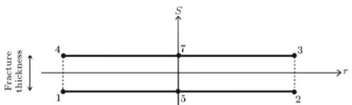
The thermo-elastic consolidation problem has been solved by Aboustit et al. [28] and also by Lewis et al. [36]. In this case, a column of linear elastic material is subjected to a unit surface pressure and a constant surface temperature of T = 50_{. Figure 4 shows the}

nite element mesh of the problem. The pore pressure is kept equal to zero at the top surface; everywhere else, the boundaries of the soil are sealed and insulated (i.e. no uid or heat ow is permitted). The parameters used in the analysis are summarized in Table 1 and the time steps used in the analysis are shown in Table 2. Almost the same temporal discretization shown in Table 2 was used in both studies by Aboustit et al. [28] and Lewis et al. [36], because this discretization scheme provided good agreement with the analytical solution for `isothermal' consolidation problems [37].

All components in the coecient matrix shown in Equation 40 are included in this analysis, except [K31] and [K23]. This is done for reasons of comparison

with the results of Aboustit et al. [28] and Lewis

Figure 4. Plane strain thermo-elastic consolidation.

et al. [36], in which these two matrices are set to zero. At the beginning of the analysis, a nine-point integration scheme was used to reduce oscillation in the results. However, since no signicant improvement was observed, a four-point integration scheme was employed.

The results are shown in Figures 5 to 7. Figure 5 shows that displacements at nodes 7, 27 and 37 agree well with the results obtained by Lewis et al. [36], except that the peak values are a little higher. After the peak, displacements become negative (i.e. heave). The same result is reported by Lewis et al. [36] for values after the peak. Figure 6 shows the variation of calculated pore pressure, which clearly indicates the dissipation of pore pressure with time. However, the results of this study show that the rate of pore pressure dissipation is slower than that reported by Lewis et al. [36]. It should be noted that calculating pore pressure is the most dicult part of the analysis, since it is very sensitive to time increment t and oscillation may occur at early times. Figure 7 demonstrates an excellent match between the calculated temperature in this study and those given by Lewis et al. [36]. Modeling Axisymmetric Thermal

Consolidation Around a Buried Heat Source The eects of a cylindrical radiating heat source, buried in a thermo-elastic soil, were investigated by Booker and Savvidou [38], where an analytic solution for a

Table 1. Input data for thermoelastic consolidation and fracture problems. Parameters Plane Strain

Analysis

Axisymmetric Analysis

Fracture Simulation Mass coecient (kN/m.sec 2_{) 0.00 0.00 0.00}

Damping coecient (kN/m.sec 1_{) 0.00 0.00 0.00}

Soil/rock thermal expansion(1/_{C) 0:9 10} 6 _{0:203 10} 6 _{0:9 10} 6

Fluid thermal expansion (1/_{C) 0.00 0:630 10} 5 _{0:1 10} 5

Fluid compressibility (kPa 1_{) 0.00 0.00 0:5 10} 3

Soil heat capacitance (J/m3_{.C) 40.0 40.0 5.00}

Fluid heat capacitance (J/m3_{.C) 40.0 40.0 0.00}

Thermal conductivity (J/sec.m._{C) 0.20 1.03 20.0}

Soil density (ton/m3_{) 0.00 0.00 0.00}

Fluid density (ton/m3_{) 1.00 1.00 1.00}

Fluid viscosity (kPa.sec) 0:1 10 5 _{0:1 10} 5 _{0:1 10} 5

Absolute permeability (m2_{) 0:4 10} 12 _{0:4 10} 11 _{5:5 10} 12

Modulus of elasticity (kPa) 6000.0 6000.0 0:6 10+8

Poisson's ratio 0.40 0.40 0.40 Acceleration of gravity (m/sec2_{) 9.81 9.81 9.81}

Initial porosity 0.1 0.1 0.3

1.00 1.00 1.00

Table 2. Time increments for thermo-consolidation problems.

Time Increment (seconds)

Number of Time Steps 0.01 10

0.1 10

1 10

10 10

100 10

1000 10

point-heat source was numerically integrated over the surface of a cylindrical canister. Apparently, this is the only `analytical solution' available for such a problem, as reported by Lewis et al. [36] and Vaziri and Britto [39]. A number of validation tests for thermal-hydro-mechanical problems have been proposed by other investigators, e.g. Alonso and Alcoverro [40] and Alonso et al. [41] in the course of the Catsius Clay project.

The nite element mesh depicted in Figure 8 is adopted from Lewis et al. [36]. It consists of 27 elements and 106 nodes. Booker and Savvidou [38] provided an analytical solution for the case of a cylindrical heat source where a0

au =

1

4, c = 2:0 and

= 0:4, in which a0 _{is the soil thermal expansion}

coecient, is the Poisson ratio, c is the coecient of consolidation, is the coecient of thermal diusivity

Figure 5. Variation of vertical displacement in time (Symbols: From [36], Lines: Finite element model).

Figure 6. Variation of pore pressure in time (Symbols: From [36], Lines: Finite element model).

Figure 7. Variation of temperature in time (Symbols: From [36], Lines: Finite element model).

Figure 8. Finite element mesh for axisymmetric thermo-elastic consolidation problem [36].

and au = S(1 ) + w(), where S and W are

the coecients of thermal expansion for solid particles and uid, respectively, and represents the porosity. The parameters used in the analysis are summarized in Table 1. The heat source was simulated by a constant heat input of 1000.0 J for both elements at the source. Temporal discretization is shown in Table 2.

Results are illustrated in Figures 9 to 11, which show horizontal displacements, pore pressures, and temperatures at three dierent nodes, R/Ro=1, R/Ro=2, and R/Ro=5 shown in Figure 8 (Ro is the radius of the cylindrical heat source). Figure 9 indicates that displacements gradually increase up to a certain level, then, level o and remain constant when the generated pore pressures are dissipated and the temperatures have reached the steady state condition. Since changes in horizontal displacement have not been addressed in the analytical solution provided by Booker and Savvidou [38], in Figure 9 results

Figure 9. Comparison between analytical and numerical solutions for horizontal displacements (Symbols: [36], Lines: Finite element model).

Figure 10. Comparison between analytical and numerical solutions for pore pressure (Symbols: Analytical, Lines: Finite element model).

Figure 11. Comparison between analytical and numerical solutions for temperature (Symbols: Analytical, Lines: Finite element model).

of the developed nite element model are compared with those reported by Lewis et al. [36] for the same problem. Figure 10 shows the pore pressure gener-ation and dissipgener-ation caused by the radiating heat source. For R/Ro=1, the time to reach the maximum pore pressure in the numerical solution is behind the analytical one, but for R/Ro=2 and R/Ro=5, the maximum values occur at the same time and their

magnitudes are fairly close. Variation of temperature with time is shown in Figure 11, which indicates good agreement between analytical and numerical solutions. It should be emphasized that the analytical results by Booker and Savvidou [38] do not provide the exact solution for this problem, because of the dierence between a point heat source and a cylindrical heat source. Nevertheless, in their analytical solution, the determination of temperature was completely uncou-pled from that of the displacements and pore pres-sures.

The above example indicates that the results of the developed numerical model are satisfactory for coupling of the three processes: Ground deformation, uid ow, and heat transfer.

Modeling of Thermally Induced Fracture The analyses presented above illustrate the capability of the present model in simulating coupled thermal hydro-mechanical problems. In this section, the ability of the model to simulate one-dimensional fracture propagation will be examined and the node splitting feature and activation of the fracture elements will be demonstrated. Figure 12 shows the nite element mesh for the problem of thermally induced fracture in rock. As shown, the mesh consists of ten 8-node rectangular elements and four 6-8-node fracture elements. Double nodes were used in the middle row for modeling fracture propagation. Six-node fracture elements were introduced, but were not activated at the beginning of the analysis. Also, a notch was provided, where uid with high pressure and temperature was injected into the medium. A uid ux of 10 6 _m/sec

and a heat ux of 10.0 J/sec were applied inside the notch. The initial pore pressure and temperature in the material were set to zero. The material properties in this example are mentioned in Table 1. Generally, in the program, the induced stresses at the nodes are examined to determine whether the tensile or shear fracture criterion is satised. The criterion, which is

satised rst, would govern the type of fracture. For initiation of the fracture in this example, only the tensile strength criterion (for mode I fracture) has been used. Also, the stiness of the fracture elements is set to zero.

Table 3 shows fracture propagation and activation of fracture elements at dierent time steps. Figure 13 shows the variation of pore pressure at nodes 18 and 29 located at the injection boundary and at nodes 1 and 45, which are located far from the injection zone. It can be seen that pore pressures are generally higher at the injection point. Fracture elements are activated after 6 seconds. Since the permeability of the fracture elements are set to ten times higher than the permeability of the soil matrix, the pore pressure drops, because the uid suddenly nds easier paths to ow. After activation of all fracture elements, the pore pressure starts to increase again. The eects of activation of the fracture elements at nodes 1 and 45 (which are located far from the injection boundaries) are not large, as expected. Variation of pore pressure along the mesh and inside the induced fracture is depicted in Figures 14 and 15, respectively. It should be noted that, due to activation of the fracture elements, the pore pressure at some nodes becomes negative.

Table 3. Fracturing sequence in time.

Time (sec.) Split Nodes Activated Elements

1 -

-2 -

-3 -

-4 -

-5 29

-6 30 11

7 31, 32, 33 12 8 34, 35, 36, 37, 38 13, 14

9 -

-10 -

Figure 13. Variation of pore pressure at some nodes in the soil and at the fracture.

Figure 14. Variation of pore pressure in the soil due to the eect of fracturing.

Figure 15. Variation of pore pressure along the fracture.

However, these negative values decrease as the node gets closer to the right boundary where a zero pore pressure is imposed.

Figure 16 compares the variation of temperature at node 18, which is located at the injection zone, and node 1, which is located far from the injection area. As expected, temperature at the injection zone is higher. Variation of temperature along the mesh and also inside the induced fracture is illustrated in Figures 17 and 18, respectively. As the gures show, due to an injection of heated uid, the temperature

Figure 16. Variation of temperature in the soil and at the fracture.

Figure 17. Variation of soil temperature due to the injection of hot uid.

Figure 18. Variation of temperature along the fracture due to the injection of hot uid.

is gradually and smoothly increasing toward a steady state condition.

Modeling of Large Scale Hydraulic Fracture Laboratory Experiments

A joint CANMET/industry/AOSTRA funded project was undertaken by Golder Associates to perform hy-draulic fracturing experiments in a large-scale triaxial chamber. The main objectives of the study were: (1) To provide a better understanding of the mechanism

Figure 19. Schematic view of large scale triaxial chamber (not to scale) from Golders Associates Report [42-44].

of hydraulic fracture formation and propagation in uncemented oil sands under conditions of high leak-o and (2) Tleak-o determine the eect leak-of uid injectileak-on rate and, also, the inuence of dierent stress elds on the fracturing process. These experiments were carried out in a large triaxial stress chamber, shown schematically in Figure 19, which can accommodate samples of up to 1.00 meter high and 1.40 meter in diameter. Quartz sand was used in these experiments, which was saturated with a viscous uid, such as invert liquid sugar instead of oil, and injected with dyed invert liquid sugar (phases I and II) and dyed water (phase III), in order to trace the fracture. Figure 19 shows a hollow steel pipe, with an outside diameter of 33.5 mm and perforated at mid-height, which was used to simulate the injection well. Principal stresses of up to 1000 kPa could be applied independently in the vertical (v) and radial (h) directions, as illustrated in the

gure.

Lane Mountain 125 quartz sand was chosen for the laboratory tests. Its behavior was reported to be similar to oil sand, which exhibits high dilatancy and post peak softening during triaxial compression under low eective conning stresses. The specic gravity of Lane Mountain sand grain was determined to be 2.65 and its permeability was measured to be 4:56 10 3

cm/sec to water and 4:0 10 6_{cm/sec to liquid sugar.}

Boundary conditions were free draining at the top and bottom of the chamber, which were connected to a constant pressure equal to +200 kPa. No radial drainage was allowed.

At the end of each test, the sample was excavated in horizontal lifts, normally 1.5 to 3.0 cm in thickness, under black light. When each lift was completely excavated, the locations of the dye were marked with black string and, then, a normal photograph was taken under normal light [42-44].

In this study, test 4 of phase II experiments was selected for numerical modeling. The sample dimensions and position of instrumentation are shown in Figures 20 and 21. Two permeability tests carried out on the saturated sample gave permeability values of 4.9 and 4.6 Darcys. Horizontal and vertical boundary tractions of 600 kPa and 400 kPa, respectively, were applied on the sample, with a back pressure of 200 kPa to keep the sample fully saturated. The K0(= h0=v0)

value was equal to 2 for this test, which indicated that horizontal fracture planes were expected. In this test, 250 ml of dyed liquid sugar were injected into the test sample in 8.3 seconds (30 ml/sec.).

A nite element mesh comprised of 704 elements (260 eight-node rectangular elements and 444 six-node fracture elements) with 1562 six-nodes (including the double nodes) was used. Due to the axial symmetry

Figure 20. Plan view of instrumentation around the injection zone.

Figure 21. Sample dimensions and position of piezometers for test #4 of phase 2 of the experiments.

of the problem, only half the sample was analyzed, as shown in Figure 22. The boundary conditions were: Bottom boundary: Fixed in the horizontal and

vertical directions, free drainage, Top boundary: Free, free drainage,

Left boundary: Fixed in the horizontal direction, no drainage allowed,

Right boundary: Free, no drainage allowed.

An important aspect of the coupling process is nding an appropriate value for time increment, t, suitable for all eld equations. Due to the high speed of stress waves in soil/rock, the time increment in the equilibrium equation should be small enough to capture the behavior of soil/rock accurately. On the other

Figure 22. Finite element mesh and boundary conditions for modeling test 4 of phase 2.

hand, the time increment cannot be very small because the coupled analysis of the consolidation phenomenon requires that t be larger than some certain value in or-der to avoid instability and spurious oscillations [45,46]. The time increment for this analysis was chosen to be one second.

An axisymmetric analysis was carried out consid-ering the linear elastic behavior for sand with an elastic modulus equal to 41050 kPa and a Poisson ratio of 0.25. These values were obtained from small scale triaxial tests on Lane Mountain sand. The permeability of the fracture elements was considered to be 100 times greater than the surrounding soil matrix (100 ksoil). In

this analysis, nodal coordinates were not updated and a nominal thickness equal to 2 mm was considered for the fracture elements. This is close to the width of the real fractures in oil sands, which is 3 to 5 mm [13]. A list of the parameters used in the analysis is summarized in Table 4.

The test was simulated by injecting uid at the perforated area of the wellbore. An injection rate of 30 ml/sec in this test is equal to an injection ux of 0.0052 m/sec when divided by the perforated area. The variation of pore uid pressure at the injection zone is shown in Figure 23. Although the calculated peak pressure is slightly higher than the measured pressure, the overall behavior is very similar. The initial slopes of the two curves are dierent; this is because, in the nite element analysis, the stresses were examined at the end of each time step to identify the possibility of fracture. For instance, if the time increment is 1 second, no fracturing will occur until the end of the time increment. Obviously, in reality, fractures can

Table 4. List of parameters for modeling of thermo-elastic consolidation and hydraulic fracture problems.

Parameters

Hydraulic Fracture Problem Mass coecient (kN/m.sec 2_{) 0.00}

Damping coecient (kN/m.sec 1_{) 0.00}

Soil/rock thermal expansion (1/_C)

-Fluid thermal expansion (1/_C)

-Fluid compressibility (kPa 1_{) 0:3 10} 5

Soil heat capacitance (J/m3_.C)

-Fluid heat capacitance (J/m3_.C)

-Thermal conductivity (J/sec.m._C)

-Soil density (ton/m3_{) 2.0}

Fluid density (ton/m3_{) 1.33}

Fluid viscosity (kPa.sec) 1:49 10 3

Absolute permeability (m2_{) 4:48 10} 12 _{4:48 10} 10

Modulus of elasticity (kPa) 41050.0 Poisson's ratio 0.25 Acceleration of gravity (m/sec2_{) 9.81}

Initial porosity 0.48

1.00

Figure 23. Comparison between calculated and measured pore pressures (piezometer: At injection zone).

occur in a fraction of second, resulting in a higher rate of ow and lower pressure.

As seen in Figure 23, there is a jump in the pore pressure at the beginning of injection, followed by a fairly constant pore pressure during the injection. At the end of injection, both calculated and measured curves show a decline in pore pressure, which represents the consolidation phenomenon.

Pore pressures at the piezometers, installed at a distance of 75 mm from the injection pipe (Figures 20 and 21), are compared to the numerical solution in

Figure 24. Comparison between pore pressure variation of lab experiment and numerical model at the piezometer (100 mm above the injection zone).

Figures 24 and 25. Piezometers were installed at three levels, but the lower one did not show a signicant change in pore pressure. A good agreement between the numerical results and measured values in the laboratory can be observed.

The fracture pattern obtained from the numerical model is shown in Figure 26. The sequence shows the fracture pattern at the onset of injection, 4 seconds af-ter starting injection, 8 seconds afaf-ter starting injection (end of injection), and at 30 seconds. The numerical model showed a fracture zone, which gradually

ex-Figure 25. Comparison between pore pressure variation of lab experiment and numerical model at the piezometers (100 mm below the injection zone).

Figure 26. Pattern of fracture propagation from numerical model.

panded with injection. The actual fracture pattern ob-served in the laboratory is shown in Figure 27. Despite the fact that Ko=2.0, neither the numerical model nor

the experimental results showed the anticipated planar fracture. Studies on pore pressure distribution inside the medium indicated that fracture occurs at places with higher pore pressure. In other words, the contours of higher pore pressure can approximately determine the zone of fracturing [47].

Fracture Propagation in an Elastoplastic Material

In petroleum engineering, it is known that the com-pressibility of oil sand is nonlinear at low stresses (e.g. [14] ). In geotechnical terms, this basically means that the stress-strain behavior of oil sand is nonlinear and its bulk modulus (stiness) varies with changes in stress. Some researchers have considered a nonlinear elastic (hyperbolic) model for simulating this behavior [48], while others have proposed an elasto-plastic constitutive model (e.g. [49]). In this study, in order to evaluate the eects of soil failure on fracture patterns in isothermal conditions, an associated Mohr-Coulomb model was employed. This model is capable of simulating high dilation, which is an important characteristic of oil sand. In this model, the following

Figure 27. Fracture pattern form laboratory experiment reproduced form Golder Associate Report [43].

parameters were used:

Cp= 0; Cr= 0;

p= 38; r= 38;

E = 41050 kPa; = 0:25;

where Cp is the peak cohesion, Cr is the residual

co-hesion, p represents the peak friction angle, rmeans

the residual friction angle and E and represent the modulus of elasticity and Poisson ratio, respectively.

Boundary tractions of 600 kPa horizontal and 400 kPa vertical, with 200 kPa back pressure were applied on the sample. According to the Mohr-Coulomb failure criterion, the ratio of the principal stresses at yielding is given by:

1 3

2 =

1+ 3

2 sin + C cos : (42)

For C = 0 and = 38_;

1 3

2 =

1+ 3

2 sin 38! 1

3 = 4:2:

Hence, at places where this ratio applies, soil becomes plastic and stresses and pore pressures are aected, accordingly. The pore pressure variation at the injec-tion zone is shown in Figure 28. In this gure, the results of the analysis, with dierent permeabilities for the fracture elements (500 and 1000 times greater than the permeability of the surrounding soil), are included. In general, the initial pore pressure in this case shows

Figure 28. Pore pressure variation at the injection zone with dierent permeabilities for fracture elements.

around 30% higher pore pressure compared to the elastic case. The eect of increasing the permeability of fracture elements on reducing pore pressure can be observed in this gure.

Fracture patterns for elastoplastic analysis are depicted in Figure 29. Compared to the fracture patterns of elastic analysis, they are less dispersed and the fracture zones are smaller. The numerical model, in this case, indicates that tensile and shear fractures can simultaneously occur in the hydraulic fracturing process. Despite the fact that the shear failure zone is small, the dilation characteristics of the material will generate compressive stresses in a conned condition, which can inhibit fracture growth. This explains why there is a less dispersed fracture zone in the elastoplastic analysis.

CONCLUSIONS

A fully coupled thermal hydro-mechanical fracture nite element model is developed, which is able to simulate the process of hydraulic fracturing under isothermal and non-isothermal conditions. The mod-eling of large scale hydraulic fracturing laboratory experiments in uncemented porous materials, such as sand, has provided results, which are in agreement with experimental observations. In this model, the

Figure 29. Fracture pattern with associated Mohr-Coulomb model.

importance of the amount of pore pressure and its distribution is emphasized in the process of hydraulic fracturing in uncemented porous materials. The frac-ture pattern is roughly similar to the contours of high pore pressure. The numerical model shows that a change in the permeability of soil and/or fractures has a drastic eect on the variation of pore pressure and the resulting fracture pattern.

The model establishes that, in uncemented porous materials, tensile and shear fractures can occur si-multaneously. The numerical model and laboratory experiments both indicate that, for uncemented porous materials, such as oil sands, a simple planar fracture is unlikely to occur and a system of multiple fractures or a fracture zone consisting of interconnected tiny cracks should be expected.

ACKNOWLEDGMENT

The authors wish to thank CANMET, Imperial Oil Re-sources Canada Ltd., Shell Canada Ltd., Japan Canada Oil Sands Ltd., AOSTRA, and Golder Associates Ltd. for providing the experimental data for this research. NOMENCLATURE

ij stress tensor at a point

Fi external load vector

Ui displacement vector i.e. hu v wiT

m0 _{mass coecient}

c0 _{damping coecient}

i; j indices taking 1, 2 and 3 representing coordinate axes

! weighting factor

nj unit vector normal to the surface

S surface boundary

V volume

0

ij eective stress tensor (tension positive)

P change in pore uid pressure

(compression positive) ij Kronecker delta

Dijkl soil/rock constitutive matrix

"kl (total) strain tensor

S coecient of thermal expansion for

soil/rock (porous matrix)

T change in temperature

density of uid

v velocity vector of owing uid G uid mass output (sink) or input

(source)

t time

r del operator

S coecient of thermal expansion for

soil/rock

P coecient of thermal expansion for

uid

T uid compressibility

"V volumetric strain

Le volumetric thermal energy ux

E internal energy per unit mass

uid density

Q energy input (source) or output (sink) per unit volume

t time

porosity of soil/rock matrix S soil/rock density

Cs heat capacity of soil/rock

f uid density

S degree of saturation

coecient of conductivity

fi volumetric ux of owing uid

g acceleration of gravity

z elevation

J mechanical equivalent of heat Cv heat capacity of uid at constant

volume

Cp heat capacity of uid at constant

pressure

T temperature

To initial temperature

REFERENCES

1. Veatch, R.W., Moschovidis, Z.A. and Fast, C.R. \An overview of hydraulic fracturing", in Recent Advances in Hydraulic Fracturing; SPE Monograph, 12, pp 2-38 (1989).

2. Zheltov, Y.P. and Khristianovitch, S.A. \On the mechanism of hydraulic fracturing of an oil-bearing stratum", Izvest. Akad. Nauk SSR, OTN, 5, pp 3-41 (in Russian) (1995).

3. Perkins, T.K. and Kern, L.R. \Width of hydraulic fractures", JPT, Trans., AIME, 222, pp 937-49 (1961). 4. Geertsma, J. and Deklerk, F.A. \Rapid method of predicting width and extent of hydraulically induced fractures", JPT, Trans., AIME, 246, pp 1571-81 (1969).

5. Nordgren, R.P. \Propagation of a vertical hydraulic fracture", SPEJ, Trans., AIME, 253, pp 306-14 (1972).

6. Clifton, R.J. and Abou-Sayed, A.S. \A variational approach to the prediction of the three-dimensional geometry of hydraulic fractures", Paper SPE 9879 presented at the 1981 SPE/DOE Low Permeability Symposium (1981).

7. Clifton, R.J. \Recent advances in the three dimen-sional simulation of hydraulic fracturing", Develop-ments in Mechanics, Proc. 19th Mid-Western Mechan-ics Conference, Ohio State U., Columbus, 13, pp 311-319 (1985).

8. Advani, S.H., Lee, T.S. and Lee, J.K. \Three dimen-sional modeling of hydraulic fractures in layered media: Part I- nite element formulations", Journal of Energy Resources Technology, 112, pp 1-19 (1990).

9. Advani, S.H. and Lee, J.K. \Finite element model sim-ulations associated with hydraulic fracturing", SPEJ, Trans., AIME, 22, pp 209-218 (1982).

10. Settari, A. and Raisbeck, J.M. \Fracture mechanics analysis in in-situ oil sand recovery", JCPT, pp 85-94 (1979).

11. Settari, A. and Raisbeck, J.M. \Analysis and nu-merical modeling of hydraulic fracturing during cyclic steam stimulation in oil sands", JPT, pp 2201-2212 (1981).

12. Atukorala, U.D. \Finite element analysis of uid induced fracture behavior in oil sand", M.Sc. the-sis, Dept. of Civil Engineering, University of British Colombia (1983).

13. Settari, A., Kry, P.R. and Yee, C.-T. \Coupling of uid ow and soil behavior to model injection into uncemented oil sands", JCPT, 28(1), pp 81-92 (1989). 14. Settari, A. \Physics and modeling of thermal ow and soil mechanics in unconsolidated porous media", SPE 18420, pp 155-169 (1989).

15. Settari, A., Ito, Y. and Jha, K.N. \Coupling of a fracture mechanics model and a thermal reservoir sim-ulator for tar sands", JCPT, 31(2), pp 20-27 (1992). 16. Frydman, M. and Fontoura, S. \Numerical modeling

of borehole pressurization", International Journal of Rock Mechanics and Mining Sciences, 34(3-4) (1997). 17. Ouyang, G., Carey, G.F. and Yew, C.H. \Adaptive nite element scheme for hydraulic fracturing with proppant transport", International Journal for Nu-merical Methods in Fluids, 24(7), pp 645-670 (1997). 18. Itaoka, M., Sato, K. and Hashida, T. \Numerical

simulation of geothermal reservoir formation induced by hydraulic fracturing at great depth", Transactions-Geothermal Resources Council, pp 297-302 (2002). 19. Yang, T.H., Li, L.C., Tam, L.G. and Tang, C.A.

\Numerical approach to hydraulic fracturing in het-erogeneous and permeable rocks", Key Engineering Materials, 243-244, pp 351-356 (2003).

20. Reynolds, M., Shaw, J. and Pollock, B. \Hydraulic fracture design optimization for deep foothills gas wells", Journal of Canadian Petroleum Technology, 43(12), pp 5-10 (2004).

21. Lu, L.J., Sun, F.C., Xiao, H.H. and An, S.F. \New P3D hydraulic fracturing model based on the radial ow", Journal of Beijing Institute of Technology (En-glish Edition), 13(4), pp 430-435 (2004).

22. Cook, B.K., Lee, M.Y., DiGiovanni, A.A., Bronowski, D.I., Perkins, F.D. and Williams, J.R. \Discrete el-ement modeling applied to laboratory simulation of near well-bore mechanics", International Journal of Geomechanics, 4(1), pp 19-27 (2004).

23. Carter, R.D. \Appendix to: Optimum uid charac-teristics for fracture extension", by G.C. Howard and C.R. Fast, Drill and Prod. Prac., API 267 (1957). 24. Zienkiewicz, O.C. and Taylor, R.L., The Finite

Ele-ment Method, 4th Ed., 2, McGraw-Hill (1991). 25. Zienkiewicz, O.C., Chan, A.H.C., Pastor, M.,

Schre-er, B.A. and Shiomi, T. Computational Geomechan-ics, with Special Reference to Earthquake Engineering, Chapter 3, John Wiley & Sons (1998).

26. Christian, J.T. \ Two and three dimensional con-solidation", in Numerical Methods in Geomechanical Engineering, C.S. Desai and J.T. Christian, Eds., pp 399-426, London, McGraw-Hill (1977).

27. Johnston, P.R. \Finite element consolidation analysis of tunnel behavior on clay", Ph.D. Thesis, Stanford University (1981).

28. Aboustit, B.L., Advani, S.H. and Lee, J.K. \Vari-ational principles and nite element simulations for thermo-elastic consolidation", Int. J. Num. Anal. Meth. Geomech., 9, pp 49-69 (1985).

29. Thomas, G.W., Principles of Hydrocarbon Reservoir Simulation, Tabir Publishers (1977).

30. Pratts, M. \Thermal recovery", SPE Monograph No., (1982).

31. Pak, A. \Numerical modeling of hydraulic fracturing", Ph.D. Thesis, Department of Civil and Environmental Engineering, University of Alberta, Canada (1997). 32. Daneshy, A.A. \On the design of vertical hydraulic

fractures", Petroleum Engineers Journal, pp 61-68 (April 1973).

33. Wiles, T.D. and Roegiers, J.C. \Modeling of hydraulic fractures under in-situ conditions using a displacement discontinuity approach", Proceedings, 33rd Annual Technical Meeting of the Petroleum Society of CIM, Paper No. 82-33-70 (June 6-9, 1982).

34. Witherspoon, P.A., Wang, J.S.Y., Iwai, K. and Gale, J.E. \Validity of cubic law for uid ow in a deformable rock fracture", Water Resources Research, 16(6), pp 1016-1024 (1980).

35. Ryan, T.M., Farmer, I.W. and Kimbrell, A.F. \Lab-oratory determination of fracture permeability", Pro-ceedings of the 28th U.S. Symposium of Rock Mechan-ics, Tucson, pp 593-600 (1987).

36. Lewis, R.W., Majorana, C.E. and Schreer, B.A. \A coupled nite element model for the consolidation of nonisothermal elastoplastic porous media", Transport in Porous Media, 1, pp 155-178 (1986).

37. Sandhu, R.S. \Finite element analysis of soil con-solidation", National Science Foundation Grant No. 72-04110-A, Geotechnical Engineering Report No.6, Dept. of Civil Engineering, The Ohio State University, Columbus, Ohio (1976).

38. Booker, J.R. and Savvidou, C. \Consolidation around a point heat source", Int. J. for Numerical and Analyt-ical Methods in Geomechanics, 9, pp 173-184 (1985). 39. Vaziri, H.H. and Britto, A.M. \Theory and

applica-tion of a fully coupled thermo-hydro-mechanical nite element model", SPE, 25306 (1992).

40. Alonso, E. and Alcoverro, J., Catsius Clay Project. Calculations and Testing of Behavior of Unsaturated Clay as Barrier in Radioactive Waste Repositories, ENRESA Technical Publication 10/99 (1999). 41. Alonso, E. et al., Febex. Proportional

Thermo-Hydro-Mechanical (THM) Modeling of In-Situ Test, ENRESA Technical Publication 09/98 (1998).

42. Golders Associates Ltd. \Laboratory simulation and constitutive behavior for hydraulic fracture propaga-tion in oil sands, phase I", Project No. 902-2013 (1991). 43. Golder Associates Ltd. \Laboratory simulation and constitutive behavior for hydraulic fracture propaga-tion in oil sands, phase II", Project No. 912-2055, (1992).

44. Golder Associates Ltd. \Laboratory study of hydraulic fracture propagation in oil sands, phase III", Project No. 932-2005 (1994).

45. Gatmiri, B. and Magnin, P. \Minimum time step criterion in FE analysis of unsaturated consolidation: Model UDAM", Proc. 3rd European Spec. Conf. on Num. Meth. in Geo. Eng., Manchester, UK (1994). 46. Song, E.X. \Time step size in nite element analysis

of consolidation", Proc. 3rd European Spec. Conf. On Num. Meth. in Geo. Eng., Manchester, UK (1994). 47. Pak, A. and Chan. D.H. \A fully implicit single phase

T-H-M fracture model for modeling hydraulic frac-turing in oil sands", Journal of Canadian Petroleum Technology, 43(6), pp 35-44 (2004).

48. Vaziri, H.H. \Nonlinear temperature and consolidation analysis", Ph.D. Thesis, Department of Civil Engineer-ing, University of British Columbia (1986).

49. Wan, R., Chan, D.H. and Kosar, K.M. \A constitutive model for the eective stress-strain behavior of oil sands", Pet. Soc. CIM, Paper No. 89-40-66, 40th ATM of CIM, Ban (1989).