Modified fixed-grid finite element method in shape ‎optimization problems based on gradientless method

Sharif University of Technology

Transactions B: Mechanical Engineering www.scientiairanica.com

Modied xed-grid nite element method in shape

optimization problems based on the gradientless

method

M. Heshmati

_{, F. Daneshmand}

_{and Y. Amini}

a. Department of Mechanical Engineering, Kermanshah University of Technology, Kermanshah, Iran.

b. Department of Mechanical Engineering, McGill University, Canada, H3A 2K6; Department of Bioresource Engineering, McGill University, Canada, H9X 3V9.

c. School of Mechanical Engineering, Shiraz University, Shiraz, Iran.

Received 13 February 2012; received in revised form 6 January 2013; accepted 4 November 2013

KEYWORDS Shape optimization; Fixed-grid nite element method; Gradientless method; Stress concentration.

Abstract. This paper presents a methodology for solving shape optimization problems where the unknown is the shape of the problem domain. The proposed algorithm is based on minimization of the stress along the design boundary calculated by the Modied Fixed Grid Finite Element Method (MFGFEM). Using MFGFEM eliminates mesh adaptation and re-meshing processes, as needed in the standard nite element method, and reduces the analysis cost signicantly. In this study, a new approach for computing the stiness matrix of boundary intersecting elements is also presented and the optimal shape of the problem domain is obtained via a simple optimization algorithm. The performance of the proposed approach is investigated for shape optimization problems. It is concluded that the results of the present method are in good agreement with other analytical and nite element solutions.

© 2014 Sharif University of Technology. All rights reserved.

1. Introduction

Shape optimization problems are associated with nd-ing the optimum prole of a component to improve the behavior of a mechanical system and minimize some properties, e.g. the weight of the body or high stress concentrations near the corners. Many investi-gations have been carried out and various structural optimization methods have been proposed for dierent optimization problems [1].

Conventional shape optimization methods are based on using the Finite Element Method (FEM) and a set of elements formed from the boundary of the problem domain. A direct relationship is then created

*. Corresponding author. Tel.: +98 937 3154288; Fax: +98 831 7267530

E-mail address: [email protected] (M. Heshmati)

between the problem boundary and the nite element meshes and any changes in the domain boundary will also be produced in the computational meshes. The drawback of this strategy is clear: Signicant boundary changes can necessitate the adaptation or regeneration of the mesh, as it no longer provides a correct representation of the medium. Therefore, in the standard shape optimization methods based on FEM, re-meshing cannot be avoided during the optimiza-tion process if accurate analysis is to be guaranteed, especially for design problems with large changes in shape [2]. These factors incorporate a considerable amount of ineciency in the shape optimization meth-ods based on FEM.

An interesting approach to decrease FEM de-pendency on conventional mesh in shape optimization problems is to use the Fixed Grid Finite Element Method (FGFEM) [3-10] and eXtended Finite Element

Method (XFEM) [11,12]. Both FGFEM and XFEM use a xed non-boundary-tted grid to perform a nite element analysis. In FGFEM, the problem domain is covered with uniform nite elements, and a homogenization technique [3] is used to compute the stiness matrix for boundary intersecting elements. The problem domain is discretized with uniform or non-uniform nite elements in XFEM, and the step function is used to carry out integration over boundary intersecting elements [12]. It has been shown that the FGFEM and XFEM are eective in approximating the strain and stress eld by their low requirements of time and computational resources. Though the above mentioned methods are equipped with excel-lent remesh-free properties and avoid cumbersome remeshing processes, the homogenization procedure and step function used in FGFEM and XFEM re-sult in an inaccurate representation of the problem domain and decreases the accuracy of numerical so-lution [4,5,9].

The integration over discontinuous elements has already been treated by several authors and has been applied in multiphase problems [13]. In the present study, basic modications are introduced in the original FGFEM and a new approach, called Modied FGFEM (MFGFEM), is introduced to encounter the boundary intersecting elements. The modication deals with stiness matrix computation of boundary intersecting elements by introducing material coordinates (r; s) that map the internal part of the boundary intersecting element to the rectangular or triangular master element when the internal part of the boundary element is a rectangle or triangle. A new formulation is also pre-sented for mapping the internal part of the boundary when the internal part of the boundary intersecting element is a pentagon.

It should be noted that the stress gradient infor-mation must also be determined through a sensitivity analysis in the structural optimization problems to minimize stress concentrations [14-19]. Since the sensi-tivity calculation time is usually high when the number of design variables is large, a gradientless approach is used in this paper. The gradientless approaches [20-27] do not use stress derivatives for determining optimal geometries. It is well-known that the convergence rate is independent of the number of design variables in these approaches, and they are particularly appro-priate for minimizing stress concentrations in shape optimization problems with a large number of design variables. The underlying strategy for these methods is to achieve a constant or nearly constant stressed design boundary by adding material where stresses are `high' and removing it where stresses are `low'. This strategy has been shown to be consistent with the aim of minimizing the peak stress [22-27].

In the present study, the modied xed-grid

method, based on a gradientless approach for shape optimization of components and for minimizing stress concentration, is developed to overcome drawbacks in solving shape optimization problems with FEM gradient-based methods. Cubic splines are also used in the proposed method to model the shape of the design boundary and the optimal shape of the design bound-ary with constant stress is achieved iteratively. The validity and performance of the method are demon-strated by solving numerical examples and comparing the results of the present analysis with those reported in the literature.

The paper is organized as follows: First, the de-sign parameterization is described and then the notion of non-boundary tted grids is presented. The original FGFEM is described followed by an explanation of MFGFEM. After that, the application of boundary conditions is discussed and the numerical integration of a Galerkin weak form is presented. Finally, the opti-mization approach is described and numerical examples are conducted. The results obtained are also compared with analytical or numerical solutions.

2. Design parameterization

Several methods are available in representing the boundary geometry of the structure. Most researchers use the nodal coordinates of the discrete nite element model as design variables [25,27]. However, it is not suitable for the xed-grid solver, since node locations for the analysis remain unchanged throughout the optimization process.

Various types of parametric spline are commonly used for representing the local shape of geometric mod-eling. The cubic spline curves and cubic B-spline curves are as certain varieties of cubic spline function. In the cubic spline representation, the cubic spline curve is expressed in terms of the coordinates of control points and their corresponding tangents, whereas, in the B-spline [9-10] representations, the curve is represented in terms of control points of a polygon. However, when the curve passes through a set of given points, the cubic spline function, which has two continuous derivatives everywhere and possesses minimum mean curvature, is a useful representation of the design boundary. The B-spline curve is particularly useful where the curve is tted by interactive manipulation.

In this paper, cubic spline curves are selected to represent the design boundary. Because a cubic spline is a piece-wise cubic polynomial curve that has a smooth shape, the movement of a point on the line can be controlled precisely and the control points are part of the generated curve. Waldman et al. [27] tested the suitability of using a typical cubic spline interpolation on optimal shoulder llet shapes and found good results.

3. Non-boundary-tted meshes

In the shape optimization problems based on the stan-dard nite element method, the problem domain must be divided into a set of boundary tted elements with predened shapes. The elements are used for shape function construction and numerical integration. The main drawbacks of these boundary tted elements are the diculties that arise during the mesh generation period. Although there are many automatic mesh generation techniques, the generation of an acceptable boundary tted mesh for bodies with a moving bound-ary is not a simple task.

Another strategy for the numerical solution of shape optimization problems is the use of non-boundary tted meshes. In this strategy, it is not necessary for the elements to coincide with domain boundaries and, therefore, the boundaries can intersect the elements. The use of non-boundary-tted meshes in the analysis of shape optimization problems reduces the mesh generation costs, because the mesh generation process is performed without considering the boundary movement. In the same way, using non-boundary-tted meshes in the shape optimization problems reduces analysis costs signicantly. A typical non-boundary-tted mesh is shown in Figure 1. As can be seen from this gure, the intersection of elements with boundaries causes the production of elements, some portions of which are located outside the problem domain. These elements, in this paper, are called Boundary Intersecting Elements (BIE). The elements located completely inside the problem domain are named Internal Elements (IE) and the others are named External Elements (EE). The collection of IE and BIE is considered an active element set. As shown in Figure 1, the nodes are also divided into three categories: Internal Nodes (IN), External Nodes (EN), and External Boundary Nodes (EBN) which locate outside the domain boundary; this type of nodes lie on the corners of boundary intersecting elements. The collection of IN and EBN is considered an active node set.

Figure 1. A non-boundary-tted mesh and classication of nodes and elements.

4. Fixed grid nite element method

The original FGFEM uses the idea of the application of non-boundary-tted grids in the nite element solution of the problems. In this method the homogenization technique is used for the formulation of boundary inter-secting elements [3]. In the homogenization technique, it is assumed that the problem is not restricted by the original domain boundaries, and the material is distributed over the entire space with the assumption that the density and stiness of the media is a function of space. In other words, it is assumed that the stiness of IE is equal to the original material, but that the stiness of EE is very low compared to the stiness of IE. With these assumptions, the stiness of BIE is a value between the stiness of IE and EE corresponding to the area fraction of the internal part of BIE. In this approach, if Ci is the elasticity tensor of IE, Ce is the

elasticity tensor of EE; the elasticity tensor of BIE is written as:

Cb= rCi+ (1 r)Ce; r = A_Ai; (1)

where A and Ai are the total area and area of the

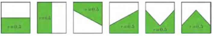
internal part of the BIE, respectively, and, therefore, r fraction. This representation of BIE causes some inaccuracy in the formulation of BIE because only the area fraction is used for the formulation of BIE and the orientation of the boundary, with respect to the element and the shape of the internal part of the element, is not introduced in the formulation of BIE. Figure 2 shows examples of 6 dierent BIE which intersect the boundary in 6 dierent congurations. The area fraction, r, for all these elements is equal and, from the view point of the homogenization technique, the stiness matrices of all these elements are the same. This causes an inaccurate representation of boundary intersecting elements.

5. Modied xed grid nite element method In this paper, some modications on the formulation of BIE are implemented to improve the accuracy of the stiness matrix and application of boundary conditions. The following sections explain these modi-cations.

5.1. Governing equations

Thepagebreak[3] governing equations for the static deformations of body, , with boundary , are as

Figure 2. Examples of dierent BIEs with same area fraction.

follows:

r: + b = 0 in ; (2) u = u on u; (3)

t = :n = t on t: (4)

In these equations, u is the displacement vector and b is the body force. The domain boundary, , is divided into two parts, u and t, which represent

the boundaries with essential and natural boundary conditions, respectively, where u \ t = 0 and u [ t = . Vectors u and t are the prescribed

displacements and traction forces, respectively, which are applied on the domain boundaries. n is the unit outward normal vector on the boundary. The total potential energy of a continuous system can be written as follows [28]:

= S L_{; (5)}

in which S _{is the strain energy and} L _{is the work}

done by external forces. We have:

S ₌1

2 Z

T_{"d; (6)}

L₌Z

uT_{bd +}Z

t

uT_{td +}Xml i=1

uT_(x

i)Ft: (7)

Fiis the external concentrated force applied at point xi,

m1is the total number of point forces, u is displacement

vector, is stress vector and " is strain vector. For 2D case, these values are dened as:

u = [uxuy]T; (8)

= [xyxy]T; (9)

" = ["x"yxy]T: (10)

The stress strain relation for a linear elastic material without residual stress and strains can be dened using elasticity matrix C as follows:

= C": (11)

5.2. Essential and natural boundary conditions In the presented method, the penalty function method is used only for essential boundary conditions, and the natural boundary conditions are applied via numerical integration of traction forces on the boundary. In this approach, for application of essential boundary conditions, the total potential energy of the system is

modied as:

₌S L₊1

21 Z

u

(u u)T_{(u u)d}

+1₂2 m2

X

i=1

(u(xi) ui)T(u(xi) ui); (12)

where, ui is the prescribed displacement in the point

constraint at point xi, m2 is the total number of point

constraints and 1and 2are the penalty parameters.

The use of a penalty function in the application of essential boundary conditions means that the rigid supports are actually replaced by a set of deformable supports, which are much stier than the materials used in the problem.

5.3. Discretization process

In this paper, a new approach for the construction of stiness is presented. In this approach, in contrast to traditional FGFEM, the degrees of freedom of all ENs are deleted and only the degrees of freedom of INs and EBNs remain as the unknown degrees of freedom.

In this method, IEs are treated as standard nite elements with no diculty. The strain energy of BIEs is computed using the integration of the strain energy density over the internal parts of these elements. Displacement, u(x), is approximated as:

u(x) = N(x)U; (13) where N(x) is the shape function matrix and U is the global displacement vector. The strain vector is dened using dierentiation operator B as:

= Bu = (BN) U: (14) Using Eq. (14), the stress vector can be written as:

= C" = C(BN)U: (15) _{is then obtained by substituting Eqs. (6), (7), (13),}

(14) and (15) into Eq. (12) as follows:

₌Z

UT_(BN)T_C(BN)UdZ U

T_NT_bd

Z

t

UT_NT_td Xm1 i=1

UT_NT i Fi

+1₂l

Z

u

(NU u)T_{(NU u)d}

+1₂2 m2

X

i=1

It should be noted that Ni = N(xi). Using the

minimum potential energy principle and dierentiating Eq. (16), with respect to displacement vector U, we have:

Z

(BN)T_{C(BN)d +} l

Z

u

NT_Nd

+ 2 m2

X

i=1

NT i Ni

U =

Z

NT_{bd +}Z

t

NT_td

+

mi

X

i=1

NT i Fi+ l

Z

u

NT_{ud +} 2 m2 X i=1 NT i u : (17) The above equation is a set of algebraic equations that can be solved simultaneously for the unknown vector, U. This equation can be written as:

(K + K)U = R + R; (18)

K = Z

(BN)T_C(BN)d;

K= 1

Z

NT_{Nd +} 2

m2

X

i=1

NT

i Ni; (19)

R = Z

NT_{bd +}Z

t

NT_{td +}Xml i=1

NT i Fi;

R= l

Z

u

NT_{ud +} 2

m2

X

i=1

NT

i u: (20)

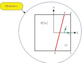
These integrals must be numerically evaluated using nonboundary-tted mesh. The intersection of the mesh with the domain boundary will divide the domain boundary into some boundary segments. These bound-ary segments are approximated by straight lines. The boundary segment of a typical boundary intersecting element (e), in Figure 1, is shown in Figure 3.

To improve the solution accuracy substantially, we develop a new scheme to calculate accurately the stiness matrix of the corresponding element. To this end, we rst determine the intersection points of the domain boundary and the element boundaries, e.g. points 3 and 4 in Figure 3, and connect these points to form the approximate boundary line. Note that the oblique boundary usually crosses the element domain without passing through the analysis nodes.

Now, we propose a new strategy to evaluate the stiness. Here, we simply work with one element denoted by e in Figure 1. First, we express the stiness

Figure 3. Typical boundary intersecting element with local coordinates (; ) and material coordinate (r; s).

matrix, ke_{, as:}

ke₌ 1 Z 1 l Z 1

(BN)T_{(; )C}

bBN(; )jJjdd: (21)

where (; ) are the element local coordinates, jJj is the Jacobian relating local coordinates (; ) and global coordinates, and BN denotes the matrix relating strains to nodal displacements. To integrate Eq. (21), we introduce the material coordinates (r; s), which maps a normalized rectangular domain, [-1,1][-1,1], to the region bounded by 1-2-3-4 in Figure 3. In Figure 3, we

i and eij!ei are the approximations of

internal and external parts of the BIE, respectively. As in the standard bilinear nite element, the element local coordinates are expressed as:

= 4 X i=1

Ni(r; s)

i

i

; (22)

where (i; i) are the coordinates of points 1, 2, 3 and

4 in Figure 3 and Ni(r; s) represent standard bilinear

functions. If !e

i becomes a triangular region, it can be

also treated by Eq. (22) as a degenerate case. Using the transformation (22), the element stiness in Eq. (21) can be written as:

ke₌ 1 Z 1 1 Z 1

(BN)T_{(; )C}

bBN(; )jJjdd

Z

wi

(BN)T_{(; )CBN(; )jJjdd}

= 1 Z 1 1 Z 1

(BN)T_{((r; s);}

where j bJj is the Jacobian relating (r; s) and (; ): b

J = _@

@r @@r @ @s @@s

: (24)

When e

ij!ie is a triangle, !iebecomes a pentagon. In

this case, Eq. (23) is not applicable and the stiness matrix for the element is obtained by subtracting the stiness of e

ij!ie from the stiness of an internal

element:

ke₌ 1

Z

1 1

Z

1

(BN)T_{(; )CBN(; )jJjdd}

Z

ij!i

(BN)T_{(; )CBN(; )jJjdd}

=

1

Z

1 1

Z

1

(BN)T_{(; )CBN(; )jJjdd}

1

Z

1 1

Z

1

(BN)T_{((r; s); (r; s))CBN)}T_{((r; s);}

(r; s))jJjjJ_jdrds;

(25) where jJ_{j results from the mapping between a}

normal-ized rectangle and e ij!ie.

As mentioned above, the domain integrals have been divided to integrations over IEs and BIEs. We emphasize that the stiness evaluation above is applied only to elements lying on the boundary. For IEs, the element stiness evaluation is exact in the proposed method. Thus, the advantages of xed grid-based methods are the fast meshing and fast formulation of the stiness matrix. It only requires small additional expenses to calculate the intersection points and element stiness matrices along the boundary of the domain.

6. Optimization approach using splines

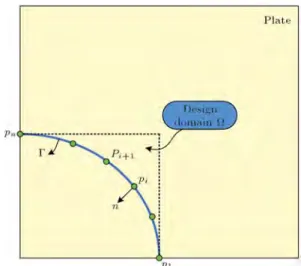
Figure 4 shows a plate with a llet with a free boundary, , on which there are a number of control points, p1; p2; ; pk. To achieve a boundary shape with a

con-stant tangential stress distribution around the bound-ary, a number of nite element based gradientless meth-ods have been proposed in the literature [25,29]. The underlying optimization algorithms for these methods are based on biological growth analogies, as elucidated by Heller et al. [25]. We add material where stresses are high and remove it where stresses are low. The amount of material added or removed at any point on

Figure 4. Geometry of plate with a llet-shaped boundary.

the boundary is taken to be directly proportional to the dierence between the local tangential stress and a suitable reference value. This process is then repeated iteratively until the boundary hoop stress is constant or nearly constant, within a prescribed tolerance. Hence, the amount to move a given point, pi, on the design

boundary (in the normal direction) is specied by the following equation [25,27,29]:

i= Ki th

th ; i = 1; 2; :::; n; (26)

where positive i indicates material addition, i is the

tangential stress at pi on the boundary, th is the

nonzero threshold boundary hoop stress, and K is an arbitrary to accelerate convergence and should be determined by trial.

The selection of the threshold stress will dene the type of optimization process and the initial boundary shape [25,27]. For example, if th is selected to be

equal to the maximum (minimum) stress, only material removal (addition) will occur. However, parameter th is initially unknown and, hence, an arbitrary

magnitude of the threshold stress has to be selected. In this paper, for the optimization problem of minimizing the stress concentration with the prescribed design domain, a xed point on the design boundary, p1, in Figure 4 is selected. This point is xed

throughout the optimization process and its stress should converge to the uniform solution stress, nally. It should be noted that the optimization logic will become much simpler if the stress at this point is selected as th [29]. Here, the cubic splines, which

are determined by a set of control points, p1; p2; :::; pk,

are used to dene the design boundary, as shown in Figure 4. The coordinates of control points are changed by simulating biological adaptive growth and the design boundary is updated accordingly. The coordinates of a

control point are updated in the following way: Y_ij+1(Pi) = Yij(Pi) + ji dji; i = 1; 2; :::; m; (27)

where Y_ij+1(Pi) and Yij(Pi) are the coordinates of

con-trol point, Pi, at the (j+1)th and jth iterations,

respec-tively. dj_i is the direction of movement for Pi (normal

direction, n, in Figure 4), m is the total number of control points, _ij is the step of Pi along the movement

direction, which can be obtained by Eq. (26).

All the control points are updated sequentially using Eqs. (26) and (27), and the splines are updated accordingly. With the new shape, the stress distri-bution along the new design boundary will become more uniform and another modied xed-grid nite element analysis is then undertaken. This process is repeated until the boundary tangential stress is constant or nearly constant. For such an iterative procedure, an appropriate function, RE, to monitor the solution convergence, can be written as clearly as RE approaches zero; the stresses become more uniform around the boundary:

RE =max_max+ min_min: (28) 7. Illustrative examples

Three numerical examples are presented and discussed here to demonstrate the accuracy and power of the boundary curve approximation and proposed shape optimization method. It must be mentioned that in the rst example, only the eciency of the MFGFEM is considered and no optimization is done.

7.1. Innite plate with a circular hole subject to a unidirectional load

In this example, the problem of 2D stress analysis around a circular hole in an innite plate under unidirectional tension was examined. The schematic diagram of the problem is presented in Figure 5. This problem is essentially a two-dimensional elasticity problem and has an analytic solution. The problem was solved in plane strain condition with a circular hole in its center. Due to symmetry, only a quarter of the problem is considered. In the cutting lines, the proper boundary conditions must be applied to simulate an in-nite media. Therefore, traction boundary conditions from the exact solution were applied on these lines. The analytic solution of this problem can be written in the following form [30]:

u =1 + v_E

1

1 + vr cos + 2 1 + v

a2

r cos

+1₂a_r2cos 3 1₂a_r34cos 3

; (29)

Figure 5. Geometry of the plate with circular hole.

v =1 + v_E

v

1 + vr sin + 1 v 1 + v

a2

r sin

+1₂a_r2sin 3 1₂a_r4₃sin 3

; (30)

x=

1 a_r2₂

3

2cos 2 + cos 4

+3a_2r4₄cos 4

; (31)

y=

a2

r2

1

2cos 2 + cos 4

+3a_2r4₄cos 4

; (32)

xy=

_a2 r2

₁

2sin 2 + sin 4

+3a_2r44sin 4

: (33) The material properties are E = 2 GPa and v = 2:26. The problem is solved for 3 dierent grid resolutions. The rst grid density consists of 16 square elements, the second grid density consists of 64 square elements and the nal mesh density consists of 256 square elements. A schematic diagram of the problem domain and boundary conditions are shown in Figure 5. The relative error in energy and displacement norms is used as a measure to compare the results. The relative error in the displacement norm is calculated using the following expression:

d = R

(u

ex _unu₎T_(uex _unu_)d

R

u

exT_uexd

!1 2

; (34)

calcu-lated using:

e = R

("

ex _"nu₎T_C("ex _"nu_)d

R

"

exT_C"exd

!1 2

: (35)

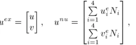
In these equations, superscripts ex and nu denote the exact and numeric values of the parameters, respec-tively. To calculate the relative errors in displacement and energy norm (Eqs. (33) and (34)), the domain integrals should be divided into integrations over IEs and internal parts of BIEs using the Gauss quadrature formula, where uex _{and u}nu _{are written as:}

uex ₌

u v

; unu ₌

2 6 6 4

4

P

i=1u e iNi 4

P

i=1v e iNi

3 7 7

5 ; (36)

where u and v are substituted from Eqs. (29) and (30). ue

i; vei are nodal displacements of the element obtained

from the present method.

The relative error norms in strain energy and displacement are presented in Figures 6 and 7 for dierent three type grid densities. It can be seen that the error in displacement and energy norms in MFGFEM for grid density #1 are 0.5% and 8.8%, for grid density #2 are 0.12% and 4.5%, and for the third mesh density are 0.04% and 2.3%, respectively. It is

Figure 6. Relative error norm in displacement for dierent numbers of element.

Figure 7. Relative error norm in strain energy for dierent numbers of element.

also obvious that the error norms in the present method are less than those obtained by FEM and FGFEM solvers.

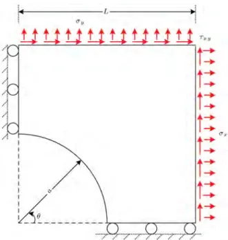
7.2. Hole in a biaxial stress eld

In this section, the benchmark structural optimization problem of a biaxial loaded plate of nite width with a hole at its center is studied. The objective of this problem is to nd out the optimal hole prole to produce the minimum Von-Mises stress on the boundary of the hole. The geometry, dimensions, boundary conditions and loading of the plate are shown in Figure 8. Only a quarter of the plate has been analyzed due to symmetry. On the symmetry lines, the proper boundary conditions must be applied to simulate the complete media. A circular arc is used to dene the initial design boundary and six control points are selected to parameterize the design boundary. After assuming the initial geometry, a xed non-boundary-tted mesh is used to solve the shape optimization of the stress concentration problem. The stress eld is obtained using the MFGFEM and the parameters are then updated via a conjugate gradientless algorithm. This process is continued until achieving convergency. A typical mesh and an initial guess for the hole prole are shown in Figure 9.

To display the results, a polar coordinate system is used, in which = 0 and = 90 show points B and A, respectively (Figures 8 and 9). Point A is the xed point and the stress at this point is selected as the threshold stress.

The stress far away from the concentration zone is 38.971 MPa. It is the value of stress which would exist in the plate without a hole. Therefore, this value has been taken for normalization of the results.

Figure 8. Dimensions, loads and boundary conditions of the problem.

Figure 9. Fixed-grid mesh of one quarter of the plate with a hole.

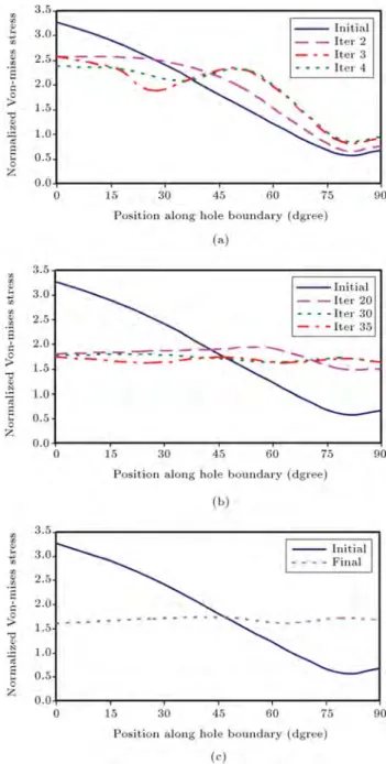
Figure 10(a)-(c) shows the normalized Von-Mises stress contours for the initial and other iterations around the hole boundary as a function of . The stress concentration around the initial hole is 3.2637 at = 0 and the minimum stress is 0.51 at = 90. It can be seen from Figure 10(a) and (b) that the convergence speed during the rst iterations is considerably higher than the last iterations, because the driving force in Eq. (26) diminishes with increasing iteration. Note that the uniform von-Mises stresses appear along the hole boundary in Figure 10(c). The ratio of the major to minor axes of the resulting ellipse is 1.951, which is close to the analytical solution for the innite plate with an ellipse, with the aspect ratio of 2:1.

The minimum possible uniform stress level along the boundary of an elliptical hole in an innite plate is 67.5 MPa [20]. In the present results, the Von-Mises stress along the design boundary is an essentially con-stant level in the range 62.87-67.502 MPa, which has good agreement with the result for the innite plate. Tekkaya and Guneri [24] investigated the same problem with the same plate geometry and boundary conditions using the biological growth method. They reported the Von-Mises stress along the design boundary is within the range 62.3- 77.9 MPa. Zhixue [29] also reported that the Von-Mises stress along the design boundary is within the range 68.98{70.30 MPa. Comparing the above results, it can be concluded that the results of the present study have extremely high accuracy.

The normalized distributions of Von-Mises stress along both the initial and nal hole boundaries are shown in Figure 10(c) as a function of . It can be noted that the stress concentration is initially 3.2637 and is reduced to 1.7404 for the optimal shape of the hole.

A summary of dierent results that are available

Figure 10. Normalized distribution of Von-Mises stress along the hole boundary.

in the literature for the same problem is presented in Table 1. The analytical solution for an innite plate and the result of our optimization for normalized maximum Von-Mises stress around the optimal hole are given. It is shown that the present normalized maximum Von-Mises stress is lower, and there is good agreement between the present result and analytical solution.

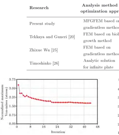
Figure 11 shows the variation of the normalized maximum Von-Mises stress with iteration number. This result clearly shows the stability and high ef-ciency of the proposed optimization method. In Figure 12, the variation of boundary hole with iteration number is also shown.

Table 1. Comparison of published results for normalized maximum Von-Mises stress around optimal hole with the present method.

Research Analysis method and

optimization approach

Normalized maximum Von-Mises stress around

optimal hole Present study MFGFEM based on

gradientless method 1.7405 Tekkaya and Guneri [20] FEM based on biological

growth method 1.998

Zhixue Wu [25] FEM based on

gradientless method 1.804

Timoshinko [26] Analytic solution

for innite plate 1.732

Figure 11. Variation of normalized maximum Von-Mises stress with iteration.

Figure 12. Variation of hole prole with iteration

In the following, the eect of an initial guess for the hole boundary on convergency of the uniform stress distribution along the optimal shape is considered. Thus, we assume the following curves for this purpose:

x a

+

y a

= 1: (37)

The above equation is plotted for dierent values of in Figure 13. It is obvious that the above equation gives a circle arc for = 2.

The normalized maximum Von-Mises stress along the initial hole boundary for dierent values of is shown in Table 2. It is obvious that the normalized maximum Von-Mises stress decreases with increasing the value of .

In Figure 14, the normalized distributions of the Von-Mises stress along the optimal hole boundary, as

Figure 13. The assumed curves for initial hole prole.

Figure 14. Normalized distribution of Von-Mises stress along the optimal hole boundary for dierent values of .

a function of , for dierent initial guesses for the hole boundary, are shown. It can be seen that for all initial guesses, the normalized stress distributions along the optimal hole boundary are the same. These results clearly show the stability and high eciency of the optimization method.

Table 2. Normalized maximum Von-Mises stress around dierent initial hole boundaries.

1 1.5 1.75 2 2.5 3

Normalized maximum

Von-Mises stress around initial hole 4.2377 3.665 3.299 3.2637 2.833 2.686

Figure 15. Geometry, dimension and boundary conditions of the shoulder llet.

7.3. Fillet plate under tension

The general geometry and notation for a symmetric at plate with a shoulder llet subject to uniaxial tension is shown in Figure 15. The objective of this optimization problem is to nd out the optimal llet shape to produce the minimum stress concentration factor. Due to symmetry, only one-half of the complete plate is modeled in the MFGFE analysis. Values of la = lb = 5l are used to keep the eect of plate length

on the state of stress in the vicinity of the llets at a negligible level. The load is assumed to be the uniform tension of 1 MPa. A wide range of llet geometries was optimized in order to produce useful design data. The values of a=b = 1:33, 1.50, 1.67, 2, and the values of l=h = 1, 2, 3, 4, 5 are considered in this example. A straight line is used to dene the initial llet shape. Point A is the xed point and the stress at this point is selected as the threshold stress. The number of control points is 20.

The iteration history of the maximum principle stress is shown in Figure 16(a)-(d). These results show that the maximum principle stress converges after a few iterations.

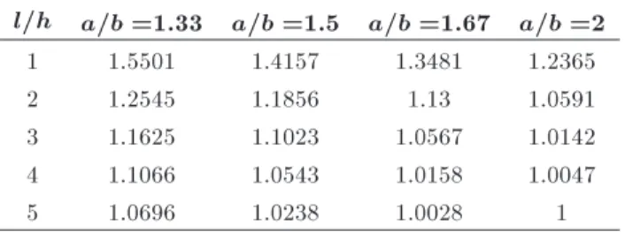
The optimum normalized maximum principal stress values (Kt) obtained for all combinations of a=b

and l=h are presented in Table 3. It can be seen that for a given a=b, the Ktvalue decreases with increasing l=h,

Table 3. The optimum normalized maximum rst principal stress values for dierent geometries.

l=h a=b =1.33 a=b =1.5 a=b =1.67 a=b =2

1 1.5501 1.4157 1.3481 1.2365

2 1.2545 1.1856 1.13 1.0591

3 1.1625 1.1023 1.0567 1.0142

4 1.1066 1.0543 1.0158 1.0047

5 1.0696 1.0238 1.0028 1

Figure 16. Variations of maximum rst principle stress with iteration number for l=h = 1 and

as expected. Also, for a given l=h, Kt decreases with

increasing a=b, which demonstrates the nite width eects. Clearly, the lowest values of Ktare, therefore,

obtained for cases where both a=b and l=h are large. It is interesting to note that in many instances, it is possible to reduce the Ktvalues very close to unity, and

a signicant reduction for Kt values is achieved. The

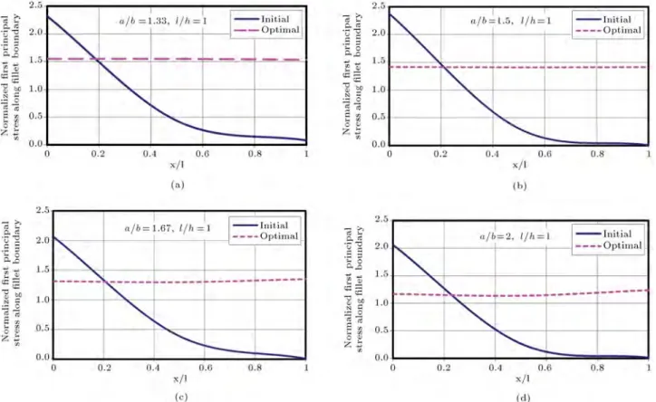
normalized maximum principle stress along both the initial and optimal shoulder llet boundaries, as a func-tion of x=l, for dierent values of a=b and l=h = 1, are shown in Figure 17(a)-(d). It is seen that the stresses are uniform along the full length of the optimal llet boundary and the reduction of the maximum principal stress along the optimal llet boundary for a=b = 1:33, 1.5, 1.67, 2 (l=h = 1) are 33.1%, 40.5%, 34.7% and 39.9%, respectively. For instance, the stresses along the optimal llet boundary for a=b = 1:67 and l=h = 1 are in the range of 1.313-1.348, while the initial line llet gives maximum stress, which is 34.7% higher. he optimal stress concentration factor with the present ge-ometry is reported in the study by Waldman et al. [27] to be 1.351, which shows excellent agreement with that achieved using the present method. This comparison demonstrates that the present method can achieve good result quality in terms of accuracy and eciency. Non-dimensional optimal tension llet shapes for dierent values of a=b and l=h are also shown in

Figure 18. Optimal non-dimensionalised tension llet shape for a=b = 1:33 and l=h = 1, 2, 3, 4, 5.

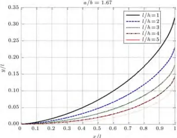
Figures 18-21. It is obvious that, as the llet gets longer (i.e. l=h gets larger), the optimal llet geometry becomes atter.

8. Conclusion

In this paper, a new method is developed for shape optimization problems using a modied xed grid FEM

Figure 17. Distributions of normalized rst principle stress along initial and optimal llet boundaries as a function of x=l for l=h = 1 and a=b = 1:33; 1:5; 1:67; 2.

Figure 19. Optimal non-dimensionalised tension llet shape for a=b = 1:5 and l=h = 1, 2, 3, 4, 5.

Figure 20. Optimal non-dimensionalised tension llet shape for a=b = 1:67 and l=h = 1, 2, 3, 4, 5.

and a gradientless approach. The objective of the shape optimization problem is to minimize the stress concentration. A new formulation for calculating the BIEs stiness matrix is also presented. The shape of the design boundary is modeled using cubic splines. The optimal shape of a design boundary with constant stress is achieved iteratively by adjusting the design boundary shape, based on a simple algorithm. Accu-rate prole shapes and associated stress concentration factors have been determined for optimal llets in shoulder plates subjected to remote tension. A signi-cant range of llet geometries has been considered. The main advantage of using non-boundary-tted meshes is to reduce the computational costs of the analysis via relaxation of the boundary conforming requirements of an acceptable mesh. This approach simplies the preprocessing stage signicantly and it is clear that preprocessing makes up a noticeable part of analysis

Figure 21. Optimal non-dimensionalised tension llet shape for a=b = 2 and l=h = 1, 2, 3, 4, 5.

cost. The only cost that should be paid for this gain is the slight increase of eort required for evaluation of the stiness matrix of boundary intersecting elements. Obviously, this additional eort is negligible when com-pared to the cost of boundary-tted mesh generation, as in standard FEM. The accuracy and convergence of the proposed method are analyzed via numerical examples and results are compared with analytic or numerical solutions. The results show good agreement with these analytic or numerical solutions.

References

1. Mackerle, J. \Topology and shape optimization of structures using FEM and BEM: A bibliography", Finite Elements in Analysis and Design, 39, pp. 243-53 (1999-2001).

2. Bennett, J.A. and Botkin, M.E. \Structural shape optimization with geometric description and adaptive mesh renement", AIAA Journal, 23(3), pp. 458-464 (1985).

3. Bensoe, M. and Kikuchi N. \Generating optimal topologies in structural design using a homogenization method", Computer Methods in Applied Mechanics and Engineering, 71, pp. 197-224 (1988).

4. Garcia, MJ. \Fixed grid nite element analysis in structural design and optimization", PhD Thesis, Aeronautical Engineering, University of Sydney, Syd-ney, Australia (1999a).

5. Garcia, M.J. and Steven, G.P. \Fixed grid nite elements in elasticity problems", Engineering Compu-tations, 16, pp. 145-164 (1999b).

6. Kim, H, Garcia, M.J., Querin, O.M., Steven, G.P. and Xie, Y.M. \Fixed grid nite element analysis in evolutionary structural optimization", Engineering Computations, 17, pp. 427-439 (2000).

7. Woon, S.Y. Querin, O.M. and Steven, G.P. \Applica-tion of the xed grid FEA method to step-wise GA shape optimization", In Proceedings of Second ASMO-UK/ISSMO Conference, Swansea, UK, pp. 265-272 (2000).

8. Garcia, M.J. and Gonzalez, C.A. \Shape optimization of continuum structures via evolution strategies and xed grid nite element analysis", Journal of Struc-tural and Multidisciplinary Optimization, 26, pp. 92-98 (2004c).

9. Edwards, C.S, Kim, H.A. and Budd, C.J. \Smooth boundary based optimisation using xed grid", 7th World Congress on Structural and Multidisciplinary Optimization (2007).

10. Lee, S., Kwak, B.M. and Kim, Y. \Smooth boundary topology optimization using B-spline and hole gener-ation",International Journal of CAD/CAM, 7(1), pp. 16-31 (2007).

11. Nicolas, M. John, D. and Ted, B. \A nite element method for crack growth without remeshing", Interna-tional Journal for Numerical Methods in Engineering, 46(1), pp. 131-150 (1999).

12. Pierre, D., Laurent, V.M., Thibault, J. and Claude, F. \Generalized shape optimization using X-FEM and level set method", IUTAM Symposium on Topological Design Optimization of Structures, Machines and Ma-terials, 137, pp. 23-32 (2006).

13. Steven, G.P. \Internally discontinuous nite elements for moving interface problems", International Journal for Numerical Methods in Engineering, 18, pp. 569-582 (1982).

14. Bletzinger, K.U., Firl, M. and Daoud, F. \Approx-imation of derivatives in semi analytical structural optimization", Comput. Struct., 86(13,14) pp. 1404-1416 (2008).

15. Par0_{s, J., Navarrina, F., Colominas, I. and Casteleiro,}

M. \Stress constraints sensitivity analysis in structural topology optimization", Comput Methods Appl. Mech. Eng., 199, pp. 2110-22 (2010).

16. Chau, L., Bruns, T. and Tortorelli, D. \A gradient-based, parameter-free approach to shape optimiza-tion", Comput. Methods Appl. Mech. Engrg., 200, pp. 985-996 (2011).

17. Qi, Xia, Tielin Shi, Shiyuan Liu, Michael Yu Wang. \A level set solution to the stress-based structural shape and topology optimization", Computers and Structures, 90(91), pp. 55-64 (2012).

18. Pedersen, P. and Laursen, C.L. \Design for minimum stress concentration by nite elements and linear pro-gramming", Journal of Structural Mechanics, 10, pp. 243-271 (1982-1983).

19. Kaye, R. and Heller, M. \Investigation of shape opti-mization for the design of life extension options for an F/a-18 airframe Fs 470 bulkhead", Journal of Strain Analysis for Engineering Design, 35(6), pp. 493-505 (2000).

20. Schnack, E. \An optimization procedure for stress concentrations by the nite element technique", Inter-national Journal of Numerical Methods in Engineering, 14, pp. 115-124 (1979a).

21. Schnack, E. and Sporl, U. \A mechanical dynamic programming algorithm for structure optimization", International Journal of Numerical Methods in Engi-neering, 3(11), pp. 1985-2004 (1986b).

22. Mattheck, C. and Burkhardt, S. \A new method of structural shape optimization based on biological growth", International Journal of Fatigue, 12(3), pp. 185-190 (1990a).

23. Mattheck, C. and Moldenhauer, H. \An intelligent CAD method based on biological growth", Fatigue Fracture Engng. Mater. Struct, 13(1), pp. 41-51 (1990b).

24. Tekkaya, A.E. and Guneri, A. \Shape optimization with the biological growth method: A parameter study", Engineering Computations, 13(8), pp. 4-18 (1996).

25. Heller, M. Kaye, R. and Rose, LR. \A gradientless nite element procedure for shape optimization", Jour-nal of Strain AJour-nalysis for Engineering Design, 34(5), pp. 323-36 (1999).

26. Tran, D. and Nguyen, V. \Optimal hole prole in nite plate under uniaxial stress by nite element simulation of Durelli's photoelastic stress minimization method", Finite Elements in Analysis and Design, 32, pp. 1-20 (1999).

27. Waldman, W. Heller, M. Chen, G.X. \Optimal free-form shapes for shoulder llets in at plates under ten-sion and bending", International Journal of Fatigue, 23, pp. 185-90 (2001).

28. Reddy, J.N., An Introduction to the Finite Element Method, 2nd Ed., McGraw-Hill, New York (1993). 29. Zhixue, Wu \An ecient approach for shape

opti-mization of components", International Journal of Mechanical Sciences, 47, pp. 1595-1610 (2005). 30. Timoshinko, S.P. and Goodier, J.N., Theory of

Elas-ticity, 3rd Ed., McGraw-Hill, New York (1970).

Biographies

Mahmood Heshmati received his BS degree in Mechanical Engineering from Razi University of Ker-manshah, Iran, in 2005, and his MS degree in Me-chanical Engineering from Shiraz University, Iran, in 2008. He is currently an assistant professor in Kermanshah University of Technology. His research elds include composite material, functionally graded material, nanomechanics, MEMS, NEMS, nonlocal elasticity, dynamic contact, vibrational analysis, plates and beam structures, and nite element analysis. Farhang Daneshmand is Associate Adjunct Profes-sor in the Department of Bioresource Engineering in

the Faculty of Agricultural and Environmental Sci-ences, and the Department of Mechanical Engineering in the Faculty of Engineering at McGill University, USA. He is also Associate Professor in the Depart-ment of Solid Mechanics in the Faculty of Mechanical Engineering at Shiraz University, Iran. His inter-disciplinary experience is related to solid mechanics, including developing a fundamental understanding of nanotubes and nanoscale biological beam and shell structures, functions and behaviors including small-scale eects using nonlocal elasticity and gradient elasticity theories, linear and non-linear vibrations and the dynamic behavior of structures (inatable

struc-tures, hydraulic strucstruc-tures, shell containers) with and without uid-structure interaction, and advanced two-and three-dimensional computational solid mechanics (Isogeometric Analysis (IA), meshless methods, xed-grid FEM).

Yasser Amini received BS and MS degrees in Me-chanical Engineering, in 2006 and 2009, respectively, from Shiraz University, Iran, where he is currently a PhD degree student. His research interests include CFD, mesh-less methods, SPH method, uid structure interaction, rareed gas ow dynamics and DSMC method.