Volume 58 (2013)
Proceedings of the
12th International Workshop on Graph Transformation
and Visual Modeling Techniques
(GTVMT 2013)
Learning Minimal and Maximal Rules from
Observations of Graph Transformations
Abdullah Alshanqiti, Reiko Heckel and Tamim Ahmed Khan
12 pages
Guest Editors: Matthias Tichy, Leila Ribeiro
Managing Editors: Tiziana Margaria, Julia Padberg, Gabriele Taentzer
Learning Minimal and Maximal Rules from
Observations of Graph Transformations
Abdullah Alshanqiti1, Reiko Heckel1and Tamim Ahmed Khan2
1amma2|[email protected]
Department of Computer Sciences, Leicester University, UK
Department of Computer and Software Engineering, Bahria University, Pakistan
Abstract: Graph transformations have been used to model services and systems where rules describe pre and post conditions of operations changing a complex state. However, despite their intuitive nature, creating such models is a time-consuming and error-prone process. In this paper we investigate the possibility of extracting rules from observations of transformations, i.e., pairs of input and output graphs re-sulting from successful transformations and individual input graphs were they have failed. From such positive and negative examples, minimal rules are extracted, to be extended by context that is present in all positive examples and missing in at least one negative example. The result is are a maximal and a required rule, jointly with the minimal rule defining the range of possible rules that could have created the ob-served transformations. We report on an implementation of the approach, evaluate its accuracy, scalability and limitations, and discuss applications to reverse engi-neering visual constructs from observations of object states of components under test.
Keywords:graph transformation, rule learning
1
Introduction
Reverse engineering is concerned with the extraction of specifications from existing systems. This can either be achieved by analysing, statically, the implementation of the system or by, dynamically, deriving the specification from observations of its behaviour. In the case of typed graph transformation, the specification is given by a type graph and a set of rules and the system’s behaviour can be represented abstractly by a transformation relation labelled by rule names. In this setting, dynamic reverse engineering means to learn rules from observed transformations.
L
m
(1)
K
(2) l
o
o r //
R m∗
Goo l∗ D r∗ //H
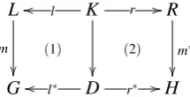
Figure 1: DPO diagram representing a rule application
set of graphs where invocations have failed. From both we hope to derive visual contracts as interface specifications for the operation.
In this paper we concentrate on the last part of the problem, the extraction of rules from exam-ple transformations. After defining more precisely the problem, we discuss several challenges and their solutions and present an algorithm for learning rules from positive and negative ex-amples generated by the AGG tool [AGG12]. To cope with the uncertainly of how well the set of examples observed can characterise the actual implementation of the operation, we derive not just one rule, but three: A minimal rule that characterises the effect, but with minimal pre-condition, a maximal rule that has as precondition the intersection of all contexts of successful transformations, and a required rule that only has context where there is evidence of its necessity. The results are evaluated and discussed, before we address related work and conclude the paper.
2
Problem
We assume the basic definitions of the algebraic double-pushout (DPO) approach over typed graphs [EEPT06]. A graph G= (V,E,s,t) consists of a setV of nodes (or vertices), a set E
of edges, and source, target functions s,t:E→V. Atype graph T Gis a distinguished graph introducing vertex and edge types. A graph morphism f :G→H is a pair of mappings fV :
GV →HV,fE :GE →HE compatible with sources and targets. An instance graph overT G is a graphGwith a graph morphismtypeG:G→T G. The category of graphs typed overT Gis calledGraphT G.
A rule is a pairL←−l K−→r Rof injective graph morphisms. In this paper we assume that
K=L∩R and l,r are inclusions. Given an instance graphG, a rule p is applied at a match
m:L→Gsatisfying the gluing conditions by deleting the image ofL\Rand adding a copy of
R\L. That means, the application is only possible if the graph patternLis mapped to Gby m
in such a way that no element inLis identified with an element inL\R, and after removing the image ofL\Rthe resulting structure is still a graph, i.e., there are no dangling edges. The result of this construction is a double-pushout diagram like inFigure 1, where the pushout on the left represents deletion and the one on the right models creation.Figure 3(A) shows a transformation rule which, when applied to the graph in the top left of (B) at the match mappingrtor1,gtog1, andhtoh, produces the graph in the top right of (B).
A graph transformation system (GTS)(P,π)consists of a set of rule namesPand a function
π assigning each name pa ruleπ(p) =L←−l K−→r R. The resulting transformation relation
In this paper we are interested in extracting rules from example transformations. More pre-cisely, we assume a type graph T G and set of rule namesP, and for each p∈P a set−→⊆p
GraphT G×GraphT Gof successful transformations and a set of6 p
−→⊆GraphT Gof failed trans-formation attempts. Our aim is to define, for each rule name p ∈P, a rule π(p) such that
p
−→⊆=⇒p , i.e., the positive examples are part of the rewrite relation and 6−→ ∩p =⇒p 1=/0, i.e., none of the negative examples is.1
Here we face a number of potential problems. First, the sets−→p and6−→p of examples may be inconsistent, i.e., there may not be a single rule pperforming all the transformations in−→p and none of those in6−→p . Second, even if such a rule exists, the sets of examples may not be varied or representative enough to derive a unique result. Third, there is a tradeoff between having enough examples to form a representative set and being able to process them in reasonable time.
We address the first problem by assuming that our examples areconsistent, generating them with the AGG tool [AGG12] for experimental purposes: Given a GTS and a start graph, rules are applied randomly to generate sets of pairs of graphs as examples to learn from. This allows us to compare the rules extracted with the original ones, as illustrated inFigure 2. Such generating graphs by AGG will simulate dynamic object extraction, by e.g. tracing a number of different sequences of system’s states at runtime.
To address the problem of ambiguity, for each p∈Pwe will provide not a single rule, but three: aminimal rulemin(p), amaximal rulemax(p), and anrequired rulereq(p), all with the same effect but differing by the additional context included in the precondition. The minimal rule able to perform a given transformation can be determined using the construction proposed in [BHE09]. For the maximal rule, we add all the context that is present in all successful exam-ples. The required rule only contains context whose necessity is confirmed by failed examples, i.e., where a failure shows that without the context present, the rule is not applicable. These three rules can assist developers to understand the range of object behaviours, with req(p)representing the best candidate to describe the functionality of the system.
To address the third problem, we have to ensure that our algorithm scales to large numbers of examples. To this end we assume that in the rules’ left-hand sides there is no disconnected context, i.e., each element that is not deleted itself is there as a node being source or target to an edge that is deleted or to be created, or is connected by an undirected path to such a node or edge. Thus, elements that are deleted or created provide us with anchor points from which all other elements can be reached. Our evaluation of scalability shows that the learning effort is linear up to about 800 pairs or graphs given as examples, but exponential in the size of the graphs.
3
Algorithm
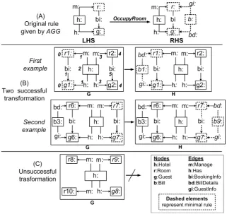
The example in Figure 3 illustrates our solution. Under (A) it shows the original rule occu-pyRoomwhich is applied randomly to generate successful pairs of graphs, shown in (B), and failed individual graphs represented in (C). The learning algorithm analyses these graphs with the purpose of discovering a rule approximating the one in (A).
1For a relationR⊆S×S, byR
Figure 2: Learning and evaluation
The process has three stages. It begins with extracting the minimal rule for each successful pair of graphs. Intuitively, for a given pair(G,H)we know thatL\R=G\HandR\L=H\G. Then, min(p) is the smallest rule satisfying these requirements [BHE09]. In the first pair of graphs in (B), the dotted nodes and edges represent the minimal rule. It is given byH\G, i.e., nodeb1:Billand its outgoing edgesbd, gi, as well as the nodes required to attach these edges, namelyr1:Roomandg1:Guest. That means, nodes in the context are part of the minimal rule if one of their incoming or outgoing edges is.
The second stage of learning is to discover the maximal rule. This requires the intersection of all successful pre-graphs, extending the minimal rule by adding to its left-hand side a repre-sentative for each graph element that occurs in all examples. Consider the two pairs of graphs given inFigure 3(B). The matches for their minimal rules are given by nodesr1,g1 andr7,g7 respectively. The intersection of their contexts include the Hotel node and the second pair of room and guest present in each case, i.e.,r2,g2 in the first rule andr6,g6 in the second, along with their connecting edges. The maximal rule, as inferred from these two examples, is therefore isomorphic to the first example.
In the third stage, the minimal rule is extended byrequiredcontexts only. To prove that context is required, we need an example that fails because this context is missing.2 Such an example is given under (C), where the match for the minimal rule exists, but there is no transformation because of the missing bi edge. This shows that the edge is required. The required rule is therefore the subrule ofOccupyRoomin (A) missing only the Hotel node and adjacent edges.
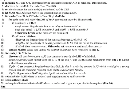
The algorithm is presented more explicitly inAlgorithm 1. As is mentioned above, successful examples produce the minimal and maximal rule, while the failures allow us to extend the mini-mal rule towards the required rule by discovering which context is necessary for the application. Rather than operating directly on the XML output of AGG, we import all graphs into a rela-tional database, seeline 1, to handle efficiently large (numbers of) graphs. This is because pars-ing and manipulatpars-ing a large number of XML instances is costly both in time and memory. A relational database provides the means to formulate complex operations on graphs as declarative
2Disregarding for now the existence of too much context in the presence of negative application conditions. 3The process at distance 5 and all nodes and edges are similar in their signatures. So which node and edge can be
Figure 3: Original rule given by AGG Vs. successful and unsuccessful graphs
Figure 4: Complex decision to define the accurate intersection3
queries. Similar motivations have led to the use of relational databases in graph transformation before, e.g., in [VFV06].
ids. The distance is the shortest path to an element in the minimal rule. InFigure 3(B) this is indicated by the numbers in the first pre-graph. The abstract id is a unique identifier in MAR.
For each successful example within the first loop inlines 7-8we confirm that its minimal rule is isomorphic to that of MAR. If this is not the case, the transformations are not all produced by the same rule, which contradicts our assumption that the examples are consistent. Once the minimal rules are matched, the next step is to discover the intersection of their additional contexts inlines 9-12. The difficulty at this point arises when matching contexts that have similar signatures.
Figure 4describes such a situation, where it is unclear which node or edge to remove to arrive at the intersection. We overcome this problem by marking the contexts and leaving the decision to the step of updating MAR after finishing the second loop inline 13.
Another difficulty is to define the starting point for matching failed graphs. In successful ex-amples, we start matching from the elements of the minimal rule. In failure cases, only individual graphsGare available. Therefore, we have to assume that each possible match of the left-hand side of MAR’s minimal rule that satisfied the gluing conditions is a possible starting point. Then we can use the same mechanism for matching as in the successful examples, but with the purpose of discovering missing context(s), seelines 14-18.
Algorithm 1Learning Graph Transformation Rules
Inputs:SSG [G,H]is a set of successful pairs of graphsand SFG [G]is a set of unsuccessful individual graphs Outputs:minRule, maxRule and requiredRule
Begin
1: initialiseSSGandSFGafter transferring all examples from GGX to relational DB structure. 2: discoverthe minRule for eachG⇒HinSSG
3: setthe distances for each node(s) and edge(s)∈GinSSG 4: letMARMax-Abstract-Rule= the smallest pair of graphs in SSG 5: for eachG and HinSSGwhereG and H6=MARdo
6: for eachnode and edge vinLHS of MAR(ascending order by distances)do 7: if v.distance= 0then
8: confirm matching the minRule as a sub-graph isomorphism such thatminG→LHS of minMARandminH→RHS of minMAR Otherwise breakas the rules are not consistent
9: ifv.distance>0then
10: discoverthe intersections of the contexts betweenLofMAR∩G
11: setpD= the possibility of deleting contexts in MAR that are out of the intersection 12: ifpD=1thenremove contextOtherwise setremove++andmark the contexts 13: update MAR()delete and update the context(s) that has been remarked inline 12 14: for eachfGinSFGdo
15: discoverall possible subsets∈fGthat can match exactly the LHS of minMAR
assume matchingeach subset to be the LHS of themin-fGand use the same mechanism fromline 9 to 12but with different conditions :
16: ifpD>0setcontext.isRequired=true inMAR.As this is a missing context in fG which would give a strong reason that the context is required to be exists to avoid such failure.
17: ifpD<0generatea NACNegative Application Conditionfor the rule 18: setminRule=MARwhere its node(s) and edge(s) must be atdistance=0 19: setmaxRule= MAR
As a result, the relationships between minimal, maximal and required rules and the original
π(p)is min(p)⊆req(p)⊆π(p)⊆max(p). The example inFigure 3illustrates the possibility
of req(p)⊂π(p)as req(p)does not containh:Hotel.
4
Evaluation
In this section, we apply our learning algorithm to the Hotel case study [HKM11]. The original system consists of nine rules, but we only use the subset ofbookRoom, freeRoom, occupyRoom, checkoutbecause we are not interested in conditions or computations on attributes. InFigure 5, a registered guest can book or free a room, adding or removingbookingInfoedges betweenRoom
andGuestnodes. If a room is booked, it can be occupied and freed by checking out.
We conduct two types of experiments, to evaluate scalability with respect to graph size and number of examples considered. Scalability is significant here because, in contrast to work on learning model transformations [Var06,BV09] our examples are not generated manually, but by observing a running implementation. That means, it may require a large number of examples to obtain enough coverage of the behaviour to allow accurate learning. We mimic this situation by generating examples using AGG.
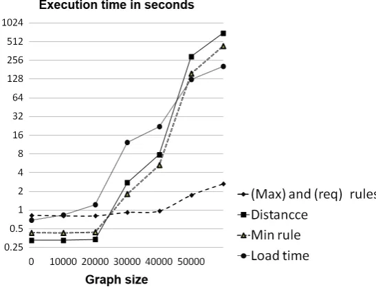
For the first experiment, we have generated 12 examples based on graphs of increasing size and, while running the algorithm, recorded the time it takes to load them into the database, construct the minimal rule, calculate the distance of each node and edge to an element in the minimal rule, derive the maximal and required rules, and the total time. The results, reported in
Table 1and visualised inFigure 6, show that significant time is spent in loading the graphs into the database, calculating distances and minimal rules, while the more sophisticated computations of maximal and required rules are less significant. This is down to an efficient representation of graphs and rules in the database, which takes time to set up but benefits subsequent steps. Since we are planning to extend the approach towards more advanced features, such as negative application conditions or multi-objects, this is a useful observation. Nevertheless, the overall effort is exponential in the sizenof the graph, very roughly 2n/500−2seconds.
Figure 5: Main rules of Hotel system:BookRoom,FreeRoomandCheckout rules
No graph size execution time (seconds)
pre post total size load minimal rule distance max+req rule total time 1 12 15 27 0.5650323 0.4280245 0.3270187 0.9730556 2.2931311 2 16 19 35 0.6020344 0.4260244 0.3280188 1.6990972 3.0551748 3 16 19 35 0.6030345 0.4290245 0.3270187 0.7990458 2.1581235 4 18 21 38 0.6200355 0.4240242 0.3290188 0.8210471 2.1941256 5 19 22 41 0.6450369 0.4250243 0.4090234 0.8120465 2.2911311 6 20 23 43 0.6550375 0.4310246 0.4170239 0.7980457 2.3011317 7 24 27 51 0.6850392 0.4320247 0.3280188 0.8190468 2.2641295 8 38 41 79 0.8370479 0.4310247 0.3280187 0.8070462 2.4031375 9 74 77 151 1.2210699 0.4390251 0.3380193 0.8060461 2.8041604 10 1126 1129 2255 12.228699 1.8081034 2.762158 0.9160524 17.715013 11 2074 2077 4151 22.084263 5.3053035 7.7954458 0.9640552 36.149068 12 12074 12077 24151 125.66019 157.04499 294.58885 1.7420996 579.03613 13 20074 20077 40151 204.91972 433.91382 698.92598 2.6491515 1340.4087 Execution time to analyse 13 successful examples is approximately 33.251 minutes 1995.0731
Table 1: Performance by graph size
Figure 6: Performance by graph size
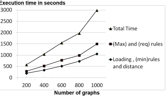
Figure 7: Performance by batch size
batch size relevant number loading, min rule, distance max+req rules total time
200 116 195.8182 89.9412 285.7594
400 238 337.6163 183.9155 521.5319
600 357 514.6824 257.8967 772.5791
800 453 729.1207 258.0947 987.2154
1000 565 1057.4894 438.11 1495.5995
Time measured in seconds
Table 2: Performance by batch size
This is important because of the trade-off between the accuracy of the rules constructed (likely to be improved with more examples of more divers context) and the effort in processing large batches. Our finding in this experiment is that the majority of examples have very similar con-texts, but a larger batch size will increase the probability of finding effective examples.
5
Related Work
to a required one using negative examples.
When considering approaches to learning model transformations [KLR+12], we have to dis-tinguish two types of transformations [MV06], i.e., in placewhere source and target have the same metamodel, as in animating object diagrams by transforming them from one state to the next, andout place, where the metamodels are different, such as when transforming UML class diagrams to relation schemata. However,in place can implementout placeby creating a joint metamodel. For learning model transformations, [DDF+11] represent input and output mod-els as meta-model instances, supporting concepts such as attributes, inheritance, aggregation, etc. Their transformations areout place, so an input-output pair does not represent the result of applying a single rule, but potentially a process consisting of several steps.
[FSB12,Var06,BV09] also propose the learning ofout placetransformation rules. Therefore, they require a mapping between metamodels to specify the relation between source and target models. Being of the in place variety, our metamodel (type graph) is always the same and no mapping is required. [LWK10] also addresses the learning ofin place model transformations. This approach is interactive, requiring user involvement to confirm the rules proposed by the algorithm. Our approach does not have direct user involvement and uses positive and negative examples for learning. More substantially, our application scenario is not one of a small num-ber of carefully hand-crafted examples, but of large numnum-bers of observations extracted from a running system. Therefore, scalability and the ability to deal with example sets providing in-complete coverage are important.
An algorithmic problem closely related to ours is graph pattern discovery. Current approaches can be classified into statistical and node signature-based solutions. Finding graph patterns by statistical means is popular in machine learning algorithms [QHJH10]. They can produce a large variance in results, depending on the frequency of a pattern. For instance, an object that is not part of the rule, but always present in the context, would be considered an important element of the rule. [QHJH10] apply decision tree learning, starting to discover matches from predefined anchor points in a hierarchical search pattern, resulting in exponential effort.
The use of node signatures can reduce this effort, but the problem remains NP-complete. [CFSV04] discusses research in exact and best graph pattern matching, most of it limited to a specific domain. A crucial point in graph or sub-graph matching is how to make nodes dis-tinguishable when they are candidates for possible matches. For example in [JMT09], a node signature for attributed graphs is based on node/edge types and node attribute(s). Our node sig-natures do not include attribute(s), but distance information, which is only available due to the construction of minimal rules before matching additional context.
6
Conclusion
rules, sometimes used as queries or property rules. For cases where the graph does not change during the transformation, the minimal rule is empty and thus all context is disconnected. Inde-pendently, rules with more advance features should be supported, including negative application conditions, multi objects, attributes, etc.
Our approach is intended for reverse engineering applications in the context of model-based testing. In such a scenario it is meaningful to consider active learning, e.g., by creating additional examples in the form of test cases and observing the system’s reaction, for example in order to verify the required context in case there are not enough negative examples.
Acknowledgement We are grateful to Neil Walkinshaw for his advice on machine learning and its use in testing.
Bibliography
[AGG12] Attributed Graph Grammar System. 2012.
http://user.cs.tu-berlin.de/∼gragra/agg/
[BHE09] D. Bisztray, R. Heckel, H. Ehrig. Verification of Architectural Refactorings: Rule Extraction and Tool Support.Proceedings of the Doctoral Symposium at the Inter-national Conference on Graph Transformation - Electronic Communications of the EASST 16, 2009.
[BMT+12] H. Brito, H. Marques-Neto, R. Terra, H. Rocha, M. Valente. On-the-fly extraction of hierarchical object graphs.Journal of the Brazilian Computer Society, pp. 1–13, 2012.
[BV09] Z. Balogh, D. Varr. Model transformation by example using inductive logic pro-gramming. International Journal - Software and Systems Modeling8(3):347–364, 2009.
[CFSV04] D. Conte, P. Foggia, C. Sansone, M. Vento. Thirty years of graph matching in pattern recognition.International journal of pattern recognition and artificial intelligence
18(03):265–298, 2004.
[DDF+11] X. Dolques, A. Dogui, J.-R. Falleri, M. Huchard, C. Nebut, F. Pfister. Easing model transformation learning with automatically aligned examples. InProceedings of the 7th European conference on Modelling foundations and applications. ECMFA’11, pp. 189–204. Springer-Verlag, Berlin, Heidelberg, 2011.
[EEPT06] H. Ehrig, K. Ehrig, U. Prange, G. Taentzer. Fundamentals of Algebraic Graph Transformation (Monographs in Theoretical Computer Science. An EATCS Series). Springer-Verlag New York, Inc., pp 12, 21,22, Secaucus, NJ, USA, 2006.
IEEE/ACM International Conference on Automated Software Engineering. ASE 2012, pp. 250–253. ACM, New York, NY, USA, 2012.
[HKM11] R. Heckel, T. A. Khan, R. Machado. Towards Test Coverage Criteria for Visual Contracts.Proceedings of the Tenth International Workshop on Graph Transforma-tion and Visual Modeling Techniques GTVMT - Electronic CommunicaTransforma-tions of the EASST 41, 2011.
[JMT09] S. Jouili, I. Mili, S. Tabbone. Attributed graph matching using local descriptions. In
Advanced Concepts for Intelligent Vision Systems - Acivs 2009. Pp. 89–99. Springer, 2009.
[KLR+12] G. Kappel, P. Langer, W. Retschitzegger, W. Schwinger, M. Wimmer. Concep-tual Modelling and Its Theoretical Foundations. In D¨usterh¨oft et al. (eds.). Chap-ter Model transformation by-example: a survey of the first wave, pp. 197–215. Springer-Verlag, Berlin, Heidelberg, 2012.
[LWK10] P. Langer, M. Wimmer, G. Kappel. Model-to-Model Transformations By Demon-stration. In Tratt and Gogolla (eds.),Proceedings of the Third international confer-ence on Theory and practice of model transformations. Lecture Notes in Computer Science 6142, pp. 153–167. Springer Berlin Heidelberg, 2010.
[MV06] T. Mens, P. Van Gorp. A Taxonomy of Model Transformation. Electron. Notes Theor. Comput. Sci.152:125–142, Mar. 2006.
[QHJH10] M. Qiu, H. Hu, Q. Jiang, H. Hu. A New Approach of Graph Isomorphism Detection Based on Decision Tree. InEducation Technology and Computer Science (ETCS), 2010 Second International Workshop on. Volume 2, pp. 32–35. 2010.
[Var06] D. Varr. Model Transformation By Example. InIn Proceedings of the ACM/IEEE 9th International Conference on Model Driven Engineering Languages and Systems (MoDELS/UML). Pp. 410–424. Springer, 2006.
[VFV06] G. Varr, K. Friedl, D. Varr. Implementing a Graph Transformation Engine in Rela-tional Databases.International Journal - Software and Systems Modeling5(3):313– 341, 2006.