DEVELOPMENT OF A STATIONARY DIGITAL BREAST TOMOSYNTHESIS SYSTEM FOR CLINICAL APPLICATIONS
Andrew Wallace Tucker
A dissertation submitted to the faculty of the University of North Carolina at Chapel Hill in partial fulfillment of the requirements for the degree of Doctor of Philosophy in the
Department of Biomedical Engineering.
Chapel Hill 2014
ii
© 2014iii
ABSTRACT
ANDREW WALLACE TUCKER: Development of a Stationary Digital Breast Tomosynthesis System for Clinical Applications
(Under the direction of Otto Z. Zhou)
Digital breast tomosynthesis (DBT) has been shown to be a very beneficial tool in the fight against breast cancer. However, current DBT systems have poor spatial resolution compared to full field digital mammography (FFDM), the current gold standard for screening mammography. The poor spatial resolution of DBT systems is a result of the single X-ray source design. In DBT systems a single X-ray source is rotated over an angular span in order to acquire the images needed for 3D reconstruction. The rotation of the X-ray source degrades the spatial resolution of the images. DBT systems which are approved for use in the United States for screening mammography are required to also take a full field digital mammogram with every DBT acquisition in order to compensate for the poor spatial resolution. This double
exposure essentially doubles the radiation dose to patients.
Over the past few years our research group has developed a carbon nanotube (CNT) based ray source technology. The unique nature of CNT ray sources allows for multiple X-ray focal spots in a single X-X-ray source. Using this technology we have recently developed a stationary DBT system (s-DBT) system which is capable of producing a full tomosynthesis image dataset with zero motion of the X-ray source. This system has been shown to have increased spatial resolution over other DBT systems in a laboratory setting. The goal of this thesis work was to optimize the s-DBT system, demonstrate its usefulness over other systems, and finally implement it into the clinic for a clinical trial.
iv
magnified 2D mammography and a conventional single source DBT system. Readers preferred s-DBT to magnified 2D mammography for specimen margin delineation and mass detection, these results were not significant. Using physical measures for spatial resolution the s-DBT system was shown to have improved image quality over conventional single source DBT
systems in breast tissue. A separate study showed that s-DBT could be a feasible alternative to FFDM for screening patients with breast implants. Finally, a second s-DBT system was
v
ACKNOWLEDGEMENTS
I would like to thank my advisor, Dr. Otto Zhou, for his leadership and guidance through my graduate studies. Dr. Zhou has shown a great dedication to the advancement of
mammographic imaging. His continued research into the field will one day enable breast cancer to be detected at an early stage thus saving countless lives. I would also like to thank each member of our research group that has helped me through my studies including; Laurel Burk, Jabari Calliste, Guohua Cao, Pavel Chtcheprov, Emily Gidcumb, Mike Hadsell, Christy Inscoe, Marci Potuzco, Xin Qian, Jing Shan, Jerry Zhang, and Lei Zhang. I would personally like to thank Dr. Jianping Lu and Dr. Yueh Lee, without your helpful guidance and insight into my research I would not have been able to complete this endeavor. I would also like to thank each member of my Ph.D. committee for their insight and direction. Dr. Lalush, thank you for your advisement during both my undergraduate studies at NC State and my graduate studies at UNC. I would like to give a special thanks to Dr. Etta Pisano, although I did not get to finish my
research under your advisement, I am eternally thankful for the opportunity you gave me in breast cancer research which lead me on the path to my Ph.D.
During my graduate studies I have had many collaborative efforts with our industrial sponsor, Hologic Inc. I would like to thank everyone at Hologic who has helped with implementation of my research into the clinic at UNC. I would also like to thank all of the employees in the Department of Mammography at UNC Hospitals who have helped me
vi
vii
TABLE OF CONTENTS
LIST OF TABLES ... xv
LIST OF FIGURES ... xvii
LIST OF ABBREVIATIONS ... xxiv
Chapter 1: INTRODUCTION ... 1
1.1 Dissertation Overview ... 1
1.2 Specific Aims ... 3
1.3 Dissertation Organization ... 5
REFERENCES ... 7
Chapter 2: X-RAY PRODUCTION AND INTERACTIONS IN MATTER ... 9
2.1 Overview ... 9
2.2 Discovery of X-rays ... 9
2.3 X-ray Production ...10
2.3.1 Bremsstrahlung X-rays ...10
2.3.2 Characteristic X-rays ...12
2.4 X-ray Tube Design ...13
2.4.1 The Cathode ...14
2.4.2 The Anode ...16
viii
2.4.4 Effective Focal Spot ...19
2.5 X-ray Interactions in Matter ...19
2.5.1 Photoelectric Absorption ...19
2.5.2 Rayleigh Scatter ...20
2.5.3 Compton Scatter ...21
2.5.4 Pair Production ...22
2.5.5 Attenuation Coefficient ...22
REFERENCES ...24
Chapter 3: MAMMOGRAPHIC IMAGING FUNDAMENTALS ...25
3.1 Overview ...25
3.2 The Human Breast ...25
3.2.1 Female Breast Anatomy and Positioning ...25
3.2.2 Breast Density ...27
3.2.3 Masses ...29
3.2.4 Microcalcifications ...30
3.3 Image Quality ...31
3.3.1 Contrast ...31
3.3.2 Spatial Resolution ...34
3.3.3 Noise...37
3.4 Image Interpretation ...39
ix
Chapter 4: MAMMOGRAPHIC IMAGING MODALITIES ...43
4.1 Overview ...43
4.2 Screening Mammography Modalities ...43
4.2.1 Screen Film Mammography ...43
4.2.2 Full Field Digital Mammography ...44
4.2.3 Digital Breast Tomosynthesis ...47
4.3 Adjunct Mammographic Imaging Modalities ...48
4.3.1 Ultrasound ...48
4.3.2 Magnetic Resonance Imaging ...49
4.4 Major Investigative Modality...50
4.4.1 Computed Tomography ...50
REFERENCES ...53
Chapter 5: CARBON NANOTUBE BASED X-RAY SOURCES ...56
5.1 Overview ...56
5.2 Field Emission from CNTs Versus Thermionic Emission ...56
5.3 CNT Based X-ray Sources ...59
5.4 Applications of CNT Based X-ray Sources ...62
5.4.1 Micro-Computed Tomography ...63
5.4.2 Micro-Beam Radiation Therapy ...66
5.4.3 Chest Tomosynthesis ...68
x
5.4.5 Digital Breast Tomosynthesis ...70
REFERENCES ...72
Chapter 6: STATIONARY DIGITAL BREAST TOMOSYNTHESIS ...76
6.1 Overview ...76
6.2 Motivation for a Stationary System ...76
6.3 First Prototype System ...77
6.3.1 CNT Source Array ...78
6.3.2 Detector ...78
6.3.3 Switching System ...79
6.3.4 Images ...79
6.4 Second Prototype System ...79
6.4.1 CNT Source Array ...80
6.4.2 Selenia Dimensions Components ...83
6.4.3 Images ...83
6.5 Conclusion ...87
REFERENCES ...88
Chapter 7: OPTIMIZATION OF AN S-DBT SYSTEM ...90
7.1 Overview ...90
7.2 Motivation for System Optimization ...91
7.3 Methods ...92
xi
7.3.2 Entrance Dose ...93
7.3.3 Phantom Imaging ...94
7.3.4 Image Processing and Reconstruction ...95
7.3.5 Modulation Transfer Function Calculation ...96
7.3.6 Signal Difference to Noise Ratio Calculation ...96
7.3.7 Artifact Spread Function Analysis ...97
7.3.8 Overall Image Quality Factor ...98
7.4 Results ...98
7.4.1 Modulation Transfer Function ...99
7.4.2 Signal Difference to Noise Ratio ... 100
7.4.3 Artifact Spread Function Along the Z-Axis ... 101
7.4.4 Detector Pixel Size Comparison ... 103
7.4.5 Overall Image Quality Factor ... 104
7.5 Discussion ... 105
7.6 Conclusions ... 107
REFERENCES ... 108
Chapter 8: BREAST SPECIMEN IMAGING WITH S-DBT ... 109
8.1 Overview ... 109
8.2 Motivation for Specimen Imaging ... 110
8.3 Methods ... 110
xii
8.3.2 Imaging on the s-DBT System... 111
8.3.3 Reader Study Design ... 111
8.4 Results ... 112
8.5 Discussion ... 115
8.6 Conclusion ... 117
REFERENCES ... 119
Chapter 9: HIGH RESOLUTION MICROCALCIFICATION IMAGING WITH S-DBT ... 120
9.1 Overview ... 120
9.2 Motivation ... 121
9.3 Methods ... 122
9.3.1 Stationary digital breast tomosynthesis system ... 122
9.3.2 Continuous motion digital breast tomosynthesis system... 124
9.3.3 Imaging protocol ... 124
9.3.4 Image processing and reconstruction ... 124
9.3.5 Microcalcification analysis ... 125
9.3.6 Simulated 3D modulation transfer function ... 126
9.4 Results ... 128
9.4.1 Microcalcification analysis ... 128
9.4.2 Simulated 3D modulation transfer function ... 129
9.5 Discussion ... 132
xiii
REFERENCES ... 134
Chapter 10: FEASIBILITY OF S-DBT AS A SCREENING TOOL FOR PATIENTS WITH AUGMENTATION MAMMOPLASTY ... 136
10.1 Overview ... 136
10.2 Motivation for Implant Imaging ... 137
10.3 Methods... 138
10.3.1 Augmentation Mammoplasty Models ... 139
10.3.2 Imaging Configuration ... 140
10.3.3 Image Processing and Reconstruction ... 141
10.3.4 Image Analysis ... 141
10.4 Results ... 144
10.4.1 Masses ... 145
10.4.2 Fibers ... 146
10.4.3 Spec Clusters ... 147
10.5 Discussion ... 148
10.6 Conclusions ... 149
REFERENCES ... 150
Chapter 11: CLINICAL IMPLEMENTATION OF AN S-DBT SYSTEM ... 151
11.1 Overview ... 151
11.2 Motivation for Clinical Implementation ... 151
11.3 System Construction and Installation ... 152
xiv
11.4.1 Electrical Safety ... 155
11.4.2 Radiation Safety ... 157
11.4.3 Institutional Review Board Approval ... 158
11.5 System Characterization ... 158
11.5.1 Geometry Calibration ... 159
11.5.2 Spatial Resolution ... 161
11.5.3 Current Versus Voltage Curve ... 162
11.5.4 Dose Rate ... 163
11.6 Patient Imaging ... 164
11.7 Conclusion ... 166
REFERENCES ... 167
Chapter 12: SUMMARY AND IMPLICATIONS ... 168
12.1 Overview ... 168
12.2 Summary of Research ... 169
12.2.1 Optimization of an s-DBT System ... 169
12.2.2 Breast Specimen Imaging with s-DBT ... 170
12.2.3 High Resolution Microcalcification Imaging with s-DBT ... 172
12.2.4 Feasibility of s-DBT as a Screening Tool for Patients with Augmentation Mammoplasty ... 173
12.2.5 Clinical Implementation of an s-DBT System ... 175
12.3 Implications ... 176
xv
LIST OF TABLES
Table 1: Linear attenuation coefficient for various materials at an energy of 50 keV. As the electron density increases the
probability of photon interaction increases thus the linear attenuation coefficient increases. Table is recreated from data
from Bushberg et al.22 ...23 Table 2: BI-RADS breast density classifications. Data taken from
Baker et al.35 ...28 Table 3: Typical lesions with their associated locations and
disease. Data taken from Kopans.31 ...29 Table 4: BI-RADS classifications of malignancy. Data taken from
Eberl et al.36 ...30 Table 5: MC types and their associated diagnosis. Data taken
from Baker et al.35 ...30 Table 6: Determination of TP, TN, FP, and FN base off disease
truth and diagnosis. ...40 Table 7: List of configurations and parameters that were analyzed.
Five parameters were changed in order to create different configurations; number of projection views, total angular span, entrance dose, distribution of the mAs, and detector resolution. Some configurations are described by multiple groups and therefore appear multiple times in the table. Differences in entrance dose for equal mAs values can be attributed to different source to object distances for different x-ray sources. MMOC stands for more mAs on central projections. LMOC stands for
less mAs on central projections. ...93 Table 8: Calculated results for SdNR, FHWM of the ASF, and
MTF. Data is separated into the five groups of configurations that were outlined in Section 7.3.1. The configuration with 29
projection views, a 28 degree angular span, and an even dose distribution resulted in the highest “QF” value for an exposure of 100 mAs. MMOC stands for more mAs on central projections.
LMOC stands for less mAs on central projections. ...99 Table 9: Calculated sensitivity and specificity values by modality
and reader. Values were calculated from malignancy scores. Malignancy scores from 3 to 5 were considered positive for
disease. ... 113 Table 10: Average reader preference for the shape/morphology of
masses, MC assessment, and margin assessment. Positive values represent a preference for stationary digital breast
xvi
Table 11: Results of the secondary analysis performed on the preference portion of the reader study. It was tested whether the mean preference was larger than zero using a linear mixed model
with a random intercept effect and Wald test. ... 115 Table 12: The results of the MC area calculation and ASF for all
12 individual MCs that were analyzed. FWHM stands for the full
width at half maximum of the ASF. ... 128 Table 13: Imaging configurations for each augmentation
mammoplasty model used. Each configuration corresponds to an exposure index between -35 and -25 on the Selenia Dimensions
in 2D imaging mode. ... 140 Table 14: Average number of lesions counted by reader one and
two for both imaging modalities. The configuration number is related to the implant model and will be used in later plots for ease
of implementation. ... 145 Table 15: List of major system components other than the X-ray
tube in the s-DBT system. ... 153 Table 16: Peak current draw and electrical input ratings for power
generating components of the system. ... 157 Table 17: Measured entrance dose for all three configurations and
various anode-cathode potentials. The dose rate was calculated
xvii
LIST OF FIGURES
Figure 1: Diagram of three different electron interactions in an atom where Bremmstrahlung radiation would be produced. The numbers indicate locations of X-ray production in order of increasing energy lost. The farther the electron is from the nucleus the less energy is converted to X-rays. This image is for demonstrative purposes and does not represent actual
interactions or atoms. Image is modeled after a figure from
Bushberg et al..22 ...11 Figure 2: Simulation of an energy spectrum from a X-ray source
with a tungsten target and 1 mm of tungsten filtration. The applied potential difference was 120 kVp. Both the characteristic Kα and Kβ X-ray peaks are labeled as well as the Bremmstrahlung curve. The zoomed in region shows the k edge which is the energy at which the attenuation coefficient of tungsten increases due to the
photoelectric absorption of electrons. ...13 Figure 3: Diagram of a modern X-ray tube. The major
components of an X-ray tube are the cathode, the anode, and the tube housing. The combination of the anode target angle and the anode viewing angle can change the effective focal spot on the
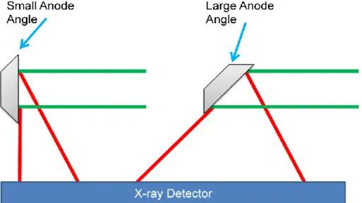
detector, thus changing the resolution of the image. ...14 Figure 4: Diagram depicting the effect of anode angle on X-ray
FOV. In the diagram, the green lines represent electron beams and the red lines represent X-ray beams. The small anode angle on the left results in a small FOV on the detector while the large anode angle on the right results in a large FOV on the detector.
Anode angles are exaggerated for demonstrative purposes...17 Figure 5: Diagram of the major and surrounding structures of the
female breast. Each structure is labeled. Image has been adapted to point to the structures. Original image is copyright Patrick J. Lynch, medical illustrator; and C. Carl Jaffe, MD,
cardiologist. And is reprinted with permission from the copyrighter
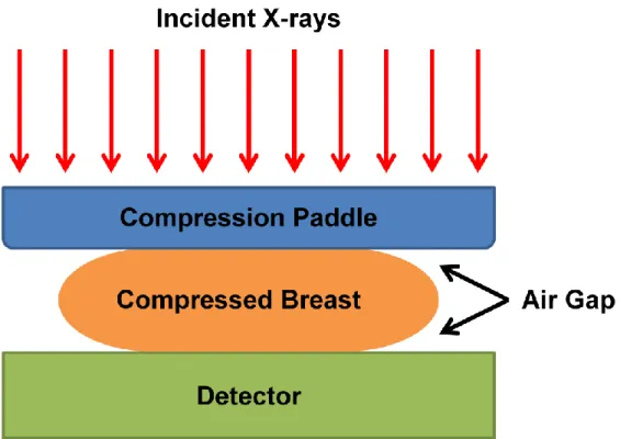
based on the Creative Commons Attribution from Wikipedia.com. ...26 Figure 6: Diagram showing the non-uniformity of breast thickness
that occurs even after compression of the breast. The air gaps in the image produce differing levels of X-ray intensity on the
detector. ...27 Figure 7: Example 2D projection radiographs of breasts with each
BI-RADS density classification. Moving from left to right the densities become more dense. This image is reprinted with
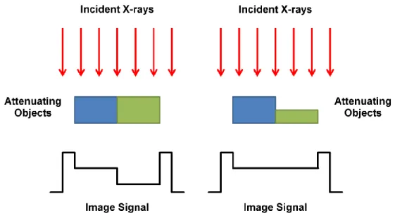
permission from Dr. Cherie Kuzmiak from UNC Hospitals. ...28 Figure 8: Demonstration of the effect of the attenuation coefficient
xviii
attenuate twice the amount of X-rays at the given energy than the blue object. The image on the Left shows that when the objects have the same thickness contrast between the two objects can be seen. However, the image on the Right shows that if the green object has half the thickness of the blue object there is no contrast between the two. This is for demonstrative purposes and does not
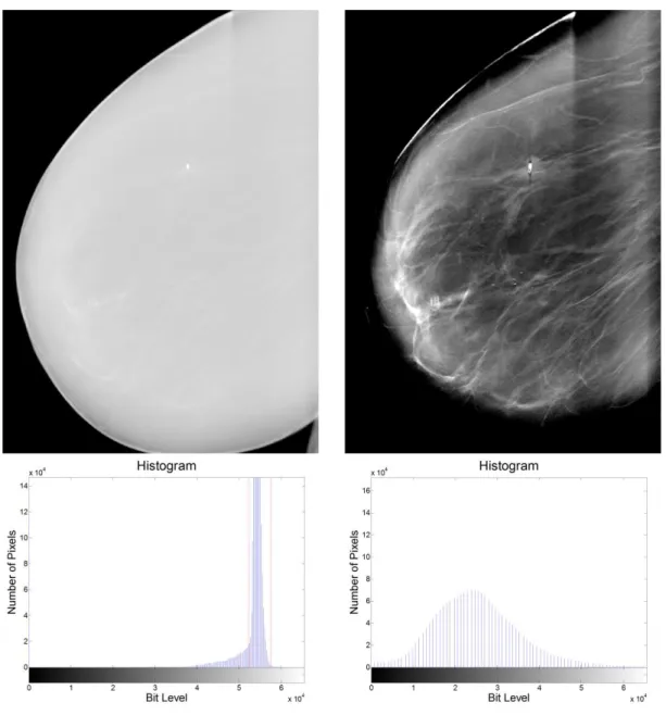
necessarily represent an actual imaging system. ...32 Figure 9: Left - An MLO image of a breast (Above) without
adjusting the image (Below). Right - Same image (Above) with adjustment of the histogram (Below). The red bars on the original histogram show the window at which the changed histogram is
contained in. This case is greatly exaggerated. ...34 Figure 10: Illustration of the effect of radiographic magnification
on the penumbra of a non-ideal focal spot. Ideal focal spots are not possible in X-ray tubes so this effect is visible in every
radiographic imaging system. ...37 Figure 11: A ROC curve that shows a system that has an
accuracy of 50%. If such a system existed, a random guess of diagnosis would give you the same results as diagnosing based
off the system...41 Figure 12: Schematic of a typical CNT based X-ray source.
Where "C" is the cathode structure, "G" is the gate electrode, "F1" and "F2" are focusing electrodes, "A" is the anode, "Vgc" is applied
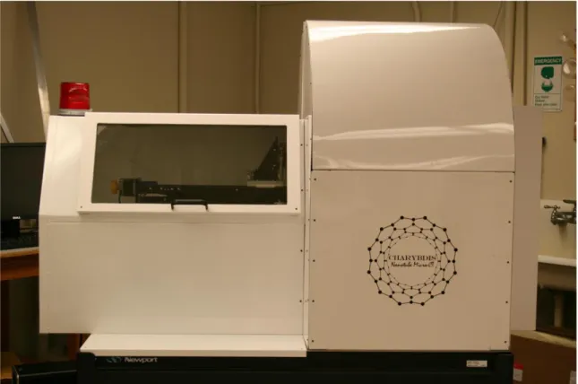
gate cathode voltage, and "Vanode" is the applied anode voltage. ...60 Figure 13: Image of the final design of the CNT based micro-CT
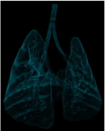
system, Charybdis. ...63 Figure 14: A 3D visualization of the lungs of a mouse imaged on
the CNT based micro-CT system. ...64 Figure 15: Left - Reconstruction of a micro-CT dataset of a
mouse which was gated to both the cardiac and respiratory cycle. All four chambers of the heart are visible. Right - Reconstruction of a micro-CT dataset of a mouse pup using the non-contact
sensor. ...65 Figure 16: Image of the desktop CNT based MRT system. ...67 Figure 17: Histological image of microbeam DNA damage in a
mouse brain with human brain tumor. Cell staining was done with
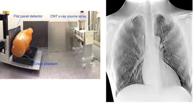
γ-H2AX labeling four hours after radiation. ...68 Figure 18: Left - Image of the prototype stationary chest
tomosynthesis system. Right - Reconstruction slice of a chest
xix
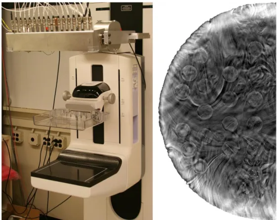
Figure 19: Left - Image of the prototype s-DBT system. Right -
Reconstruction slice of a breast phantom using the s-DBT system. ...71 Figure 20: First prototype s-DBT system. ...77 Figure 21: The X-ray spectrum of the first prototype s-DBT
system. The Mo/Mo anode filter combination produces
characteristic peaks at 17.48 and 19.61 keV. ...78 Figure 22: Reconstruction slices of a breast phantom from the
first prototype s-DBT system. The slices are at the heights of (a) 6
mm, (b) 11 mm, (c) 16 mm, and (d) 21 mm. ...79 Figure 23: Image of the second prototype s-DBT system. ...80 Figure 24: X-ray spectra of the second prototype s-DBT system at
40 keV peak energy. The characteristic peaks of the W/Al anode filter combination are at higher energies than 40 keV and therefore
do not appear in the spectra. ...81 Figure 25: Above - Gate-cathode voltages for the CNT source
array at a cathode current of 43mA. The average value was
approximately 1.4 kV. Below - Measured nominal focal spot sizes.
The average focal spot size was found to be 0.64x0.61 mm. ...82 Figure 26: Plot of the transmission rates of each X-ray source in
the prototype. The average transmission rate is 61%. ...83 Figure 27: Left - Schematic of the structures contained in the
ACR mammography accreditation phantom. Right - Schematic of
the target slab in the BR3D tomosynthesis phantom. ...84 Figure 28: Projection images from beam N14 (Left), 000 (Middle),
and P14 (Right) of the ACR phantom from the s-DBT prototype.
Images were taken at 30 kVp and 100 mAs total exposure. ...85 Figure 29: Reconstruction slice of the ACR phantom dataset.
When using fidelity display all fibers and masses are visible in this
dataset and four groups of specs. ...85 Figure 30: Projection images from beam N14 (Left), 000 (Middle),
and P14 (Right) of the BR3D phantom from the s-DBT prototype. There is a large amount of tissue overlap present in the images
which will be removed in the reconstruction slices. ...86 Figure 31: Reconstruction slice of the ACR phantom dataset.
Compared to the projection images Figure 30 most of the underlying and overlying tissue has been removed in the
xx
Figure 32: Left: Schematic of simulated masses MCs and fibers located in the ACR phantom. Analysis was conducted on the masses and MCs. Right: ACR phantom reconstructed slice
acquired using the s-DBT system. ...95 Figure 33: Left: Plot of an oversampled LSF and the
corresponding Gaussian fitted LSF which was used for MTF calculations. Right: MTF of the LSF with the value at 10%
highlighted. The MTF was found to be around 4.2 cycles per mm for a detector with a 140 µm pixel size (2x2 binning mode). Since there is no x-ray source motion in an s-DBT system the MTF is found to be primarily dependent on the detector pixel size, and
independent of other system parameters (see Figure 38). ... 100 Figure 34: Left: Magnified view of 2 mm mass found in the ACR
phantom. The SdNR of the mass and the surrounding background was calculated for each configuration. Right: Magnified view of the 0.54 mm speck cluster found in the ACR phantom. ASF analysis was completed on all specks in the
cluster for each configuration. ... 101 Figure 35: The plot of the SdNR versus total entrance dose
shows a linear increase of the SdNR with entrance dose within the dose range examined. A linear fit was applied to the dataset and
plotted. ... 101 Figure 36: Plot of the ASF of an angular span of 14 degrees
versus an angular span of 28 degrees with the same number of projection images and total entrance dose. Both the raw data and the fitted data are shown. The 14 degree span resulted in a much broader ASF due to the lack of information in the projection
space. ... 103 Figure 37: Results comparing the FWHM of the ASF and the total
angular span of the projection images. A smooth fit was also applied to the data and plotted. A very noticeable trend can be seen which shows that an increased angular span results in a
better artifact spread function. ... 103 Figure 38: Plot of the MTFs for the 70 µm pixel size and the 140
µm pixel size. The value of the MTF at 10% was found to be approximately 25% better for the 70 µm pixel size (5.1 cycles per
mm) when compared to the 140 µm case (4.1 cycles per mm). ... 104 Figure 39: Left - Segmented 2D radiograph of container used to
hold specimens. Right - Image of an s-DBT system with
specimen container on the detector housing. ... 111 Figure 40: Left Above - Reconstructed slice of a specimen using
xxi
the same specimen. The high spatial resolution of the s-DBT system allows for imaging of small microcalcifications. The added z-axis information allows for better visualization of MC clusters. The blue oval envelopes a cluster of large MCs and the white oval
envelopes a cluster of small MCs. ... 114 Figure 41: Left - Reconstructed slice of a specimen using an
s-DBT system. The spiculated margins and architectural distortion are more apparent along all edges compared to the 2D
mammography image of the same specimen (Right)... 115 Figure 42: Left - Reconstructed slice of a specimen using an
s-DBT system. Right - 2D mammography image of the same specimen. Biopsy needles are present in the s-DBT
reconstructions and not in the 2D mammography image. ... 117 Figure 43: Left - An image of the s-DBT system with a specimen
container on the detector housing. Right - An image of a Selenia
Dimensions. ... 123 Figure 44: Reconstruction slice of a breast specimen using the
s-DBT system. ... 125 Figure 45: Plot of the ASF for the s-DBT system (solid line) and
the Selenia Dimensions system (dashed line) from MC number 2.
A line representing the 50% cutoff is shown. ... 129 Figure 46: Left - Simulated MTF curves comparing the effect of
pixel size and focal spot size in the s-DBT system. Simulations for both a binned and full resolution detector are shown. Right - The
same curves but for the Selenia Dimensions system. ... 130 Figure 47: Above - Simulated 3D MTF for the s-DBT system with
a 0.9 mm isotropic focal spot size using a 70 µm (Left) and 140 µm (Right) detector pixel size. Middle - 3D MTF for the s-DBT system with a 0.6 mm isotropic focal spot size using a 70 µm (Left) and 140 µm (Right) detector pixel size. Below - Simulated 3D MTF for the Selenia Dimensions system using a 70 µm (Left) and
140 µm (Right) detector pixel size. ... 131 Figure 48: Comparison of MC sharpness for MCs number 7
through 12 between the s-DBT system (Above) and the Selenia Dimension system (Below). Aliasing from the large pixel size and effective focal spot size can be seen in the Selenia Dimensions images. Specimens were not imaged in the same orientation and
can therefore have artifacts in different directions. ... 133 Figure 49: Augmentation mammoplasty model under
compression. Two BR3D phantom slabs and the 200cc saline
xxii
Figure 50: Left - s-DBT reconstructed slice through the lesions of the model with the 400cc saline implant and two BR3D slabs. Right - 2D planar image of the same model. A large amount of
tissue overlap can be seen in the 2D planar image. ... 142 Figure 51: Region I Left - s-DBT reconstruction slice Right - 2D
planar image ... 142 Figure 52: Region II Left - s-DBT reconstruction slice Right - 2D
planar image ... 143 Figure 53: Region III Left - s-DBT reconstruction slice Right - 2D
planar image ... 143 Figure 54: Region IV Left - s-DBT reconstruction slice Right - 2D
planar image ... 144 Figure 55: Bar chart showing the average number of masses
counted for the 6 implant configuration for both reader one and two. The error bars represent one standard deviation. Missing
bars indicate failure to find any lesions. ... 146 Figure 56: Bar chart showing the average number of fibers
counted for the 6 implant configuration for both reader one and two. The error bars represent one standard deviation. Missing
bars indicate failure to find any lesions. ... 147 Figure 57: Bar chart showing the average number of spec
clusters counted for the 6 implant configuration for both reader
one and two. The error bars represent one standard deviation. ... 148 Figure 58: Pictorial time lapse of the Selenia Dimensions gantry
(Left), after X-ray tube removal (Center), and after CNT source
array integration (Right). ... 152 Figure 59: Picture of the electronics rack with all components
labeled. ... 153 Figure 60: Picture of the fully assembled s-DBT system in the
North Carolina Cancer Hospital at UNC Hospitals. ... 154 Figure 61: Diagram of the grounding scheme used in the s-DBT
system. ... 156 Figure 62: Room layout for the s-DBT system in the UNC-CH
Cancer Hospital. The numbers represent locations for radiation
field surveys. ... 158 Figure 63: Plots of the x locations (Above), y locations (Middle),
xxiii
locations indicated by the red stars and the interpolated locations
indicated by the blue lines. All distances are in millimeters... 160 Figure 64: Reconstruction image of the line pair phantom (Left).
Looking at the zoomed in region (Right) it can be seen that the s-DBT system using binned detector pixels produces approximately 4 line pairs/mm of resolution, which agrees with previous
measurements on the other s-DBT system.13 ... 162 Figure 65: Plot of the average I-V curves for the three
configurations used in the clinical trial and the plots for the best
and worst cathodes. ... 163 Figure 66: RCC projection images from beams N15 (Left), 000
(Center), and P15 (Right). ... 165 Figure 67: RMLO projection images from beams N15 (Left), 000
(Center), and P15 (Right). ... 165 Figure 68: Reconstruction slices from the first patient from the
RCC view (Left) and the RMLO view (Right). Images are in the plane of the large MC cluster on the left portion of the images. The grayscale values of these images are inverted compared to their respective projection images to demonstrate what is typically
xxiv
LIST OF ABBREVIATIONS
ACR American College of Radiology ASF Artifact Spread Function
BI-RADS Breast Imaging-Reporting and Data System
CC Craniocaudal
CLAHE Contrast Limited Adaptive Histogram Equalization
CNT Carbon Nanotube
CT Computed Tomography
DBT Digital Breast Tomosynthesis
DMIST Digital Mammographic Imaging and Screening Trial DNA Deoxyribonucleic Acid
ECS Electronic Control System
EHS Environmental Health and Safety FBP Filtered Back-Projection
FDA Food and Drug Administration FFDM Full Field Digital Mammography FFT Fast Fourier Transform
FOV Field of View
FWHM Full Width at Half Maximum GFCI Ground Fault Circuit Interrupter GPU Graphics Processing Unit iFFT Inverse Fast Fourier Transform IRB Institutional Review Board I-V Current-Voltage
MC Microcalcification
xxv
ML Maximum Likelihood
MLO Medio-Lateral Oblique
Mo Molybdenum
MOSFET Metal-Oxide-Semiconductor Field-Effect Transistor MQSA Mammography Quality Standards Act
MRT Microbeam Radiation Therapy MTF Modulation Transfer Function PVDR Peak-to-Valley Dose Ratio
QF Quality Factor
RT Radiation Therapy
SA Specific Aim
s-DBT Stationary Digital Breast Tomosynthesis SdNR Signal Difference to Noise Ratio
SFM Screen Film Mammography SID Source to Imager Distance TTL Transistor-Transistor Logic
UC Davis The University of California, Davis
1
CHAPTER 1: INTRODUCTION
1.1 Dissertation Overview
Breast cancer is the most common type of cancer found in women in the United States, with more than 200,000 new cases found each year.1 When the cancer is diagnosed at an early stage the five-year relative survival rate is between 83.9 and 98.4 percent. This number drops to 23.8 percent when the cancer is diagnosed at a stage at which it has already metastasized.1 Screening mammography is the current gold standard for early detection of breast cancer.2, 3 However, 2D mammography imaging lacks depth information, which can cause underlying and overlying tissue to obstruct the view of lesions. This leads to high false positive and false negative rates.4, 5
Digital breast tomosynthesis (DBT) uses multiple low dose projection images distributed over an angular span to create a pseudo-3D reconstruction of the breast. This added depth information allows for otherwise obscured lesions to become visible.6-9 The Hologic Selenia Dimensions is the only DBT system currently FDA approved for use in the United States.
Current DBT systems use a single x-ray source which is rotated over a limited angle arc. The x-ray source rotates in a continuous motion10, 11 or using a step-and-shoot motion.12 In both methods, the motion of the x-ray source can have an adverse effect on tomosynthesis
2
reduced by decreasing the rotation speed and increasing the acquisition time.14, 15 However, a long acquisition time leads to patient motion which also degrades image quality.16
We have developed a stationary digital breast tomosynthesis system by retrofitting a linearly distributed carbon nanotube (CNT) x-ray source array onto a Hologic Selenia
Dimensions DBT system.13, 17-20 The system is capable of creating a full set of tomosynthesis projection images with no x-ray source motion and a potential acquisition time of less than 4 seconds when coupled with a high frame rate detector.
Results have shown that the system resolution is increased from less than 3 cycles per mm with the Selenia Dimensions DBT system to more than 4 cycles per mm with the s-DBT system (1.08x magnification, 15 projection images, 15o angular span, 100 mAs). Accelerated lifetime measurements demonstrate an estimated x-ray tube lifetime of over 3 years in clinical service.13
The goal of this dissertation is to develop an s-DBT system for use in a clinical trial. Current clinical DBT systems in the United States require a 2D mammogram with all screening DBT exams. This doubles the radiation dose given to the patient. A 2D mammogram is
required due to the low spatial resolution of continuous motion DBT systems. An s-DBT system has shown to have better spatial resolution than a continuous motion DBT system. Starting a clinical trial on human patients takes the project a large step closer to showing if its image quality is good enough to remove the requirement for a 2D mammogram thus reducing the radiation dose given to each patient.
The secondary goal of this dissertation is to investigate the usefulness of s-DBT for imaging breast specimens and as a screening tool for patients who have undergone
3
detector. This would increase the accuracy of surgical margin assessment. Imaging breast specimens will also present the first human tissue imaged on an s-DBT system. The current practice of doing a four view mammogram on patients with implants increases the radiation dose to the patient, examination time, and patient discomfort. Using implant models it will be determined if it is possible to reduce the four views used currently to screen implant patients to two DBT views, one CC view and one MLO view, for each breast or possibly just a single s-DBT MLO view. This would reduce the amount of radiation to the patient, time of exam, and patient discomfort.
1.2 Specific Aims
SA 1: Develop a system for clinical use
In this specific aim (SA) an s-DBT system will be analyzed to determine the optimal imaging configuration. A system will then be built for use in a clinical trial involving human patients. The specific work will include: isolating imaging parameters and determining the effect of each one on image quality, comparing the image quality of various configurations using quantitative measures, constructing an s-DBT system for use in a clinical environment, and characterizing the system.
SA 1.1: Optimal configuration parameters
4
SA 1.2: System characterization and clinical implementation
An s-DBT system will be built for use in a clinical environment. After construction of the system, many system values will be characterized and optimized for use on patients. These values include: system geometry, radiation exposure rate based on kVp, X-ray field of view, spatial resolution, I-V curves, and transmission rates. The values will be implemented into the operating software and a radiologist technician will be trained to use the system.
SA 2: Demonstrate the usefulness of s-DBT
In this SA the usefulness of an s-DBT system for imaging breast specimens and for screening patients with augmentation mammoplasty will be determined. The specific work will include: collecting breast specimen images using DBT, determining the effectiveness of s-DBT as an imaging tool for breast specimens, demonstrating the increased spatial resolution of s-DBT, collecting phantom implant images with an s-DBT system and a 2D mammography system, and using the collected images to determine if s-DBT is a feasible alternative to 2D mammography for screening patients with augmentation mammoplasty.
SA 2.1: Breast specimen study
A protocol will be submitted to the UNC-CH Institutional Review Board. Upon
acceptance, patients scheduled for lumpectomy procedures at UNC hospitals will be recruited for use in the study. Images of the excised specimen are first taken on a 2D mammography system in the hospital by trained radiologist technicians. The specimen will then be transferred to our facility to be imaged using an s-DBT system and a clinical DBT system. The
5
After collection of a sufficient number of specimen images for statistical analysis, four trained readers will review the 2D mammography datasets and the s-DBT datasets. Readers will give malignancy scores for the datasets, confidence levels based on the s-DBT dataset, and assess the surgical margins. Statistical analysis will be completed by a trained biostatistician. Based on the results of the reader study, the efficacy of s-DBT as a tool for imaging breast specimens will be determined.
A secondary study will be conducted using the data collected on the clinical DBT system. The increased microcalcification visibility in s-DBT will be analyzed using human tissue.
Measurements will be made for the x, y, and z axis resolutions of both the clinical DBT system and the s-DBT system. Finally, a spatial resolution simulation will be used to show further proof of increased spatial resolution in s-DBT. Based on the results of the study, the extent of s-DBT image quality improvement will be determined.
SA 2.2: Feasibility of s-DBT as an implant screening tool
Augmentation mammoplasty models will be created using a combination of a breast tissue phantom with lesions and various sized saline and gel silicone implants. Each model will be imaged on an s-DBT system and a 2D mammography system using the same entrance dose. After collection of the data, the reconstructed images will be shown to trained radiologists. The radiologists will report the number of visual lesions for each dataset. The results will show if s-DBT is more effective than 2D mammography for an implant in the field of view image. Depending on the effectiveness it will be determined if s-DBT is a feasible tool for screening patients with augmentation mammoplasty.
1.3 Dissertation Organization
This dissertation is separated into three major sections: (1) background information, (2) scholarly research completed, (3) clinical trial preparation. Chapters 2 through 6 give
6
7
REFERENCES
1 N. Howlader, A. Noone, M. Krapcho, N. Neyman, R. Aminou, W. Waldron, S. Altekruse, C. Kosary, J. Ruhl, Z. Tatalovich, "SEER Cancer Statistics Review, 1975-2008, National Cancer Institute. Bethesda, MD," SEER website2011).
2 L. Nystrom, I. Andersson, N. Bjurstam, J. Frisell, B. Nordenskjold, L.E. Rutqvist, "Long-term effects of mammography screening: updated overview of the Swedish randomised trials," Lancet 359, 909-918 (2002).
3 S.M. Moss, H. Cuckle, A. Evans, L. Johns, M. Waller, L. Bobrow, "Effect of
mammographic screening from age 40 years on breast cancer mortality at 10 years' follow-up: a randomised controlled trial," Lancet 368, 2053-2060 (2006).
4 J.G. Elmore, M.B. Barton, V.M. Moceri, S. Polk, P.J. Arena, S.W. Fletcher, "Ten-year risk of false positive screening mammograms and clinical breast examinations," New England Journal of Medicine 338, 1089-1096 (1998).
5 T. Wu, R.H. Moore, E.A. Rafferty, D.B. Kopans, "A comparison of reconstruction algorithms for breast tomosynthesis," Med Phys 31, 2636 (2004).
6 I. Andersson, D.M. Ikeda, S. Zackrisson, M. Ruschin, T. Svahn, P. Timberg, A. Tingberg, "Breast tomosynthesis and digital mammography: a comparison of breast cancer
visibility and BIRADS classification in a population of cancers with subtle mammographic findings," European radiology 18, 2817-2825 (2008).
7 J.T. Dobbins III, D.J. Godfrey, "Digital x-ray tomosynthesis: current state of the art and clinical potential," Physics in medicine and biology 48, R65 (2003).
8 S.P. Poplack, T.D. Tosteson, C.A. Kogel, H.M. Nagy, "Digital breast tomosynthesis: initial experience in 98 women with abnormal digital screening mammography," AJR. American journal of roentgenology 189, 616-623 (2007).
9 A.P. Smith, L. Niklason, B. Ren, T. Wu, C. Ruth, Z. Jing, "Lesion visibility in low dose tomosynthesis," in Digital Mammography (Springer, 2006), pp. 160-166.
10 M. Bissonnette, M. Hansroul, E. Masson, S. Savard, S. Cadieux, P. Warmoes, D. Gravel, J. Agopyan, B. Polischuk, W. Haerer, "Digital breast tomosynthesis using an amorphous selenium flat panel detector," Proc. SPIE 5745, (2005).
11 B. Ren, C. Ruth, T. Wu, Y. Zhang, A. Smith, L. Niklason, C. Williams, E. Ingal, B.
Polischuk, Z. Jing, "A new generation FFDM/tomosynthesis fusion system with selenium detector," Proc. SPIE 7622, (2010).
12 X. Gong, S.J. Glick, B. Liu, A.A. Vedula, S. Thacker, "A computer simulation study comparing lesion detection accuracy with digital mammography, breast tomosynthesis, and cone-beam CT breast imaging," Med Phys 33, 1041-1052 (2006).
8
resolution stationary digital breast tomosynthesis using distributed carbon nanotube x-ray source arx-ray," Med Phys 39, 2090 (2012).
14 E. Shaheen, N. Marshall, H. Bosmans, "Investigation of the effect of tube motion in breast tomosynthesis: continuous or step and shoot?," Proc. SPIE 7961, (2011). 15 J. Zhou, B. Zhao, W. Zhao, "A computer simulation platform for the optimization of a
breast tomosynthesis system," Med Phys 34, 1098-1109 (2007).
16 R.J. Acciavatti, A.D. Maidment, "Optimization of continuous tube motion and step-and-shoot motion in digital breast tomosynthesis systems with patient motion," Proc. SPIE 8313, (2012).
17 X. Qian, R. Rajaram, X. Calderon-Colon, G. Yang, T. Phan, D.S. Lalush, J. Lu, O. Zhou, "Design and characterization of a spatially distributed multibeam field emission x-ray source for stationary digital breast tomosynthesis," Med Phys 36, 4389-4399 (2009). 18 G. Yang, R. Rajaram, G. Cao, S. Sultana, Z. Liu, D. Lalush, J. Lu, O. Zhou, "Stationary
digital breast tomosynthesis system with a multi-beam field emission x-ray source array," Proc. SPIE 6913, (2008).
19 O.Z. Zhou, G. Yang, J. Lu, D. Lalush, "Stationary x-ray digital breast tomosynthesis systems and related methods," US Patent No. US7751528 B2 (Jul 6, 2010 2010). 20 F. Sprenger, X. Calderon-Colon, E. Gidcumb, J. Lu, X. Qian, D. Spronk, A. Tucker, G.
9
CHAPTER 2: X-RAY PRODUCTION AND INTERACTIONS IN MATTER
2.1 Overview
Since the discovery of X-rays in 1895 by Wilhelm Conrad Röntgen, they have become an integral part of the medical field. X-rays are produced when high energy electrons are bombarded onto a high Z material. Once they strike the material, the electrons impart their energy into the high Z target mostly as heat. A very small portion of the energy is transformed into either Bremsstrahlung or characteristic X-rays. Careful consideration must be used when designing a X-ray tube. The size of the cathode and the tilt of the anode will significantly impact the spatial resolution of the X-ray system. Design of the filtration and collimation of an X-ray tube will ensure that the appropriate dose is given to a patient. Once the X-rays interact with the object that is being imaged through the processes of photoelectric absorption, Rayleigh scatter, and Compton scatter an image can be created with differing levels of contrast based on the attenuation of the materials being imaged.
2.2 Discovery of X-rays
Crookes tubes are partially evacuated glass tubes which contain an anode and cathode electrode.21 When a high voltage is applied between the two electrodes, a Townsend discharge occurs creating positive ions which are then attracted to the negative voltage of the cathode. The movement of the electrons are called cathode rays. Once they strike the cathode,
10
realized that some invisible ray was traversing through the cardboard and striking the screen. Through a series of experiments he found that these rays could traverse through a variety of items. He called them X-rays, the "X" standing for a mathematical variable that is unknown.22 Röntgen famously imaged his wife's hand using X-rays. This image is the very first use of medical imaging. Röntgen received the first Nobel Prize in Physics for his discovery of X-rays in 1901.
2.3 X-ray Production
X-rays are produced when the kinetic energy of electrons is converted into electromagnetic radiation. X-rays are typically created in a X-ray tube, which, unlike the Crookes tube used by Röntgen, produces electrons by a process called thermionic emission. Thermionic emission is the process of adding enough heat energy to electrons in a metal to overcome the work function of the metal. Once this occurs the electrons are emitted from the metal. In a typical X-ray source, a metal filament is heated (typically thoriated tungsten) in a evacuated chamber. A high voltage is applied between the metal filament and a metal surface in the tube. The filament is at a negative voltage (cathode electrode) while the surface is at a positive voltage (anode electrode). Once the voltage is applied between the cathode and anode, the emitted electrons will accelerate toward the anode with a kinetic energy (keV) proportional to the potential difference (kVp) between the cathode and anode. When the electrons strike the surface of the anode, their energy is converted into other forms. Approximately 99.5% of all energy is converted into heat through small electron collision exchanges.22 The other energy is converted into two types of X-rays: Bremsstrahlung and Characteristic.
2.3.1Bremsstrahlung X-rays
11
More energy is lost as the electron's path is closer to the nucleus resulting in higher energy photon production. Figure 1 is a diagram showing several electron interactions and the difference in photon energy due to distance differences. Since the size of an atoms nucleus is relatively small compared to the total area the electron shells take up, the probability of
producing high energy photons is small compared to producing low energy photons. The total photon output, or spectrum, from Bremstrahlung radiation increases linearly with decreased photon energy. However, the low energies of X-ray production are absorbed by the materials in the path of the X-ray in a process called filtration. More information on filtration can be found in Section 2.4.3.
Figure 1: Diagram of three different electron interactions in an atom where Bremmstrahlung radiation would be produced. The numbers indicate locations of X-ray production in order of increasing energy lost.
The farther the electron is from the nucleus the less energy is converted to X-rays. This image is for demonstrative purposes and does not represent actual interactions or atoms. Image is modeled after a
12
2.3.2Characteristic X-rays
Some electrons bombarding the anode will collide with an electron in the shell of an atom. If the energy transferred to the shell electron is higher than the binding energy of the electron then the electron could be ejected from the shell. The difference in the transferred energy and the binding energy is the amount of kinetic energy the now free electron will have. The atom has now become an ion. The resultant unstable electron shell will be filled with an outer shell electron at a lower binding energy. When the electron transitions shells, the difference in energy between the two shells can be expelled as a characteristic photon. Since the energy of the expelled photon depends on the different shell energies then every material produces a unique set of characteristic photons, hence the name characteristic. Each
13
Figure 2: Simulation of an energy spectrum from a X-ray source with a tungsten target and 1 mm of tungsten filtration. The applied potential difference was 120 kVp. Both the characteristic Kα and Kβ X-ray
peaks are labeled as well as the Bremmstrahlung curve. The zoomed in region shows the k edge which is the energy at which the attenuation coefficient of tungsten increases due to the photoelectric absorption
of electrons.
2.4 X-ray Tube Design
14
Figure 3: Diagram of a modern X-ray tube. The major components of an X-ray tube are the cathode, the anode, and the tube housing. The combination of the anode target angle and the anode viewing angle
can change the effective focal spot on the detector, thus changing the resolution of the image.
2.4.1The Cathode
15
electrons emitting from the cathode. If 1 mA of current is hitting the anode then 6.24 x 10¹⁵ electrons per second are hitting the anode. Tube currents for radiology X-ray tubes range from 100 to 1,000 mA with an exposure time as high as 100 ms. In order to change the tube current, the filament current is modulated. For most diagnostic X-ray energies the higher the filament current the higher the tube current. However, for lower tube potentials (potential difference between the anode and cathode) the tube becomes space charge limited. This most often is a problem for mammographic imaging modalities which can have tube potentials as low as 20 kVp. Once the tube potential is sufficiently high (> 40 kVp) the space charge is overcome by the tube potential.
The location that the electron beam hits the anode is called the focal spot. Focal spot size is very important in radiographic imaging due to its direct relationship with image spatial resolution. As the focal spot becomes larger the spatial resolution becomes worse. The
effective focal spot is the perceived focal spot on the detector and is what determines the spatial resolution. Although a tube could have a poor focal spot, the effective focal spot could be substantially smaller. The effective focal spot is covered in Section 2.4.4. The actual focal spot is directly related to the size of the cathode filament. Since filaments are long and thin, there is a substantial difference in the focal spot size in one direction compared to the other. To
compensate for the large focal spot size, the viewing angle of the X-ray detector is changed. The effect of the viewing angle can be seen in Figure 3. In the figure, the red dashed line shows a large viewing angle which increases the size of the effective focal spot. The green dashed line shows a small viewing angle which decreases the size of the effective focal spot. The thin direction of the cathode filament produces a much smaller focal spot, however in radiographic imaging even smaller focal spots are needed. Most cathode filaments are
16
cup voltage becomes more negative, the electrons are repelled from the cup and a thinner focal spot is created.
2.4.2 The Anode
17
A small amount of anode heat dissipation occurs because of the angle of the anode. Anode angles help reduce the size of the effective focal spot in the length direction of the cathode filament. The anode angle is the angle at which the anode is placed perpendicular to the electron beam. Different anode angles are used for different applications. Small anode angles produce small effective focal spots but result in an increase in the heel effect. The heel effect is when emitted X-rays travel through the anode on their path to the X-ray detector. The X-rays are attenuated by the anode and thus reduce the X-ray flux on the detector. Therefore, removing the area of X-ray radiation affected by the heel effect is important. When a small anode angle is used the useful area of the beam is reduced and therefore results in a smaller X-ray field of view (FOV) on the detector. Figure 4 demonstrates the effect of the anode angle on the X-ray FOV.
Figure 4: Diagram depicting the effect of anode angle on X-ray FOV. In the diagram, the green lines represent electron beams and the red lines represent X-ray beams. The small anode angle on the left results in a small FOV on the detector while the large anode angle on the right results in a large FOV on
the detector. Anode angles are exaggerated for demonstrative purposes.
2.4.3 Tube Housing
18
X-ray shielding. Since X-rays are produced in every direction when the tube is on, it is very important to shield patients and operators from unwanted radiation. Very dense materials are used around the vacuum housing to absorb unwanted radiation. The Food and Drug
Administration (FDA) limits the amount of radiation that penetrates this shielding to 100 mR/hr at a distance of 1 m from the focal spot.22
19
The X-ray collimator limits the FOV of the X-ray beam to the X-ray detector. FDA regulations limit the amount of radiation that can pass outside the FOV of the detector. A collimator consists of four sides of highly attenuating metal. The four sides can be adjusted in order to limit the beam to the appropriate area on the detector. More advanced collimators are used in radiation therapy systems to change the trajectory of the X-ray beams to limit the radiation exposure to normal tissue.
2.4.4 Effective Focal Spot
The effective focal spot of an imaging system is directly related to the spatial resolution of images. A smaller effective focal spot results in higher resolution images. The factors
effecting the effective focal spot are: the actual focal spot size, the anode angle, and the viewing angle. The focal spot size and viewing angle were covered in Section 2.4.1 while the anode angle was covered in Section 2.4.2. All of these factors convolved together will give the effective focal spot.
2.5 X-ray Interactions in Matter
In order for a X-ray based imaging system to produce usable images, some amount of X-ray radiation must be absorbed by the item being imaged. Variations in the absorption of different materials give contrast to X-ray images. Other forms of X-ray interaction with matter include scattering and pair production. The four major forms of X-ray photon interactions and matter are: (1) photoelectric absorption, (2) Rayleigh scatter, (3) Compton scatter, and (4) pair production.
2.5.1 Photoelectric Absorption
20
equal to the energy of the incident photon minus the binding energy of the electron. If the ejected electron was occupying an inner shell, then the vacancy in the shell will be filled by an outer shell electron. The difference in binding energies of the two electron shells will be released as either a characteristic X-ray or as an Auger electron. An Auger electron occurs when the binding energy difference is transferred to an outer shell electron. If the energy is higher than the binding energy of the electron then it will also be ejected with a kinetic energy equal to the impending energy (from the first binding energy difference) minus the binding energy of the Auger electron. After production of the Auger electron or characteristic X-ray, there is now another open position in an electron shell and the process could happen again. This will continue in a cascade from the inner shell to the outer shell. The probability of photoelectric absorption occurring is approximately proportional to the following equation:
Equation 1:
Where "Ppa" is the probability of photoelectric absorption per unit mass, "Z" is the atomic number of the absorbing material, and "E" is the energy of the incident photon. Analyzing this equation shows that higher atomic number elements will have a higher probability of
photoelectric absorption for a particular photon energy. This equation also shows why the field of mammography utilizes low energy photons for imaging. The effective atomic number of different breast tissues is between 5 and 6.27 which would require a very low photon energy to keep the probability of absorption high.
2.5.2 Rayleigh Scatter
21
they begin to oscillate another photon of equal energy but in a different direction is ejected from the atom. This particular type of scattering has a very low probability of occurring at most diagnostic energy levels. It accounts for less than 5% of all X-ray interactions above 70 keV.22 However, Rayleigh scatter becomes more of a problem for mammographic energies. At 30 keV the probability increases to 12%.22
2.5.3 Compton Scatter
Unlike Rayleigh scatter, Compton scatter is the dominant form of X-ray interaction in matter for the majority of diagnostic X-ray energies. Above approximately 300 keV, Compton scatter is the only attenuation interaction that occurs for soft tissue until pair production begins at around 3,000 keV. For energies above approximately 30 keV, Compton scatter is more prevalent than photoelectric absorption for soft tissue. In Compton scatter, the incident photon imparts enough energy to overcome the work function of the atom and ejects the electron with some kinetic energy. The incident photon has not lost all its energy, so it continues on in a separate trajectory. This type of interaction most often occurs for outer shell electrons. Total energy is conserved so the energy of the incident photon is equal to the energy of scattered photon plus the energy of the ejected electron plus the binding energy of the electron. The energy of the scattered photon can be calculated from the following equation:
Equation 2:
22
Scatter on a radiographic image can be significant with respect to the total contrast to the image. The scatter to primary ratio is the amount of detected photons from scattered interactions to the amount of unscattered photons. In radiography, scatter to primary ratios can range from 0.4 to 20.28, 29 There has been a lot of research conducted into reducing or
estimating the scatter in radiographic images. Many systems implement an anti-scatter grid to remove unwanted scattered photons.30 Anti-scatter grids are then sheets of highly attenuating metals which have a series of holes or lines which correspond to detector pixels and are aligned with the location of the X-ray source. Since the holes are aligned they will theoretically only allow photons which are on a direct path from the X-ray source. However, they do not remove all scatter due to secondary scatter and misalignment. They also reduce the amount of primary X-rays that are reaching the detector. In order to compensate for the loss in primary X-rays, longer exposures are required.
2.5.4 Pair Production
Pair production does not occur in the diagnostic energy range. X-ray energies higher than 1.02 MeV are required in order for pair production to take place.22 An electron-positron pair is produced when high energy X-rays interact with electric field of an atom's nucleus. The energies of the matter and antimatter pair are both 0.511 MeV, which is the rest mass energy of an electron. The positron will lose energy through excitation and ionization until it comes to rest. Once it comes to rest it will interact with an electron and produce an annihilation event will occur producing two photons which travel in opposite directions.
2.5.5 Attenuation Coefficient
23
thickness is called the linear attenuation coefficient "µ". The Beer-Lambert law shows the correlation between the linear attenuation coefficient and the number of transmitted photons:
Equation 3:
Where "I" is the number of photons exiting the material, "Io" is the number of photons incident on the material, "µ" is the linear attenuation coefficient of the material, and "x" is the distance traveled through the material. The linear attenuation coefficient decreases with increased X-ray energies for a given material unless a K-edge is present. Table 1 shows various materials and the relationship between electron density and attenuation coefficient at 50 keV. Materials with higher electron densities give higher probabilities that an incident electron will interact with the atom. Thus the likelihood of attenuation and the attenuation coefficient increases.
Table 1: Linear attenuation coefficient for various materials at an energy of 50 keV. As the electron density increases the probability of photon interaction increases thus the linear attenuation coefficient increases. Table is recreated from data from Bushberg et al.22
Material Density (g/cm3)
Electrons per Mass (e/g) x
1023
Electron Density
(e/cm3)
µ (cm-1)
Hydrogen 0.000084 5.97 0.0005 0.000028
Water vapor 0.000598 3.34 0.002 0.000128
Air 0.00129 3.006 0.0038 0.000290
Fat 0.91 3.34 3.04 0.193
Ice 0.917 3.34 3.06 0.196
Water 1 3.34 3.34 0.214
24
REFERENCES
1 W. Crookes, "On the Illumination of Lines of Molecular Pressure, and the Trajectory of Molecules," Proceedings of the Royal Society of London 28, 102-111 (1878).
2 J.T. Bushberg, J.M. Boone, The essential physics of medical imaging. (Lippincott Williams & Wilkins, 2011).
3 W.D. Coolidge, "X-ray tube," US Patent No. 1,355,126 (1920).
4 S.S.J. Feng, I. Sechopoulos, "Clinical Digital Breast Tomosynthesis System: Dosimetric Characterization," Radiology 263, 35-42 (2012).
5 B. Ren, C. Ruth, Y. Zhang, A. Smith, D. Kennedy, B. O'Keefe, I. Shaw, C. Williams, Z. Ye, E. Ingal, "Dual energy iodine contrast imaging with mammography and
tomosynthesis," SPIE Medical Imaging, (2013).
6 E. Roessl, R. Proksa, "K-edge imaging in x-ray computed tomography using multi-bin photon counting detectors," Physics in medicine and biology 52, 4679 (2007).
7 M. Antoniassi, A. Conceição, M. Poletti, "Study of effective atomic number of breast tissues determined using the elastic to inelastic scattering ratio," Nuclear Instruments and Methods in Physics Research Section A: Accelerators, Spectrometers, Detectors and Associated Equipment 652, 739-743 (2011).
8 G.T. Barnes, "Contrast and scatter in x-ray imaging," Radiographics 11, 307-323 (1991). 9 Z. Jing, W. Huda, J.K. Walker, "Scattered radiation in scanning slot mammography,"
Med Phys 25, 1111 (1998).
25
CHAPTER 3: MAMMOGRAPHIC IMAGING FUNDAMENTALS
3.1 Overview
In order to completely understand the research and work done in this dissertation, background information is needed on mammographic imaging. The following sections will cover anatomy of the breast and associated lesions of the breast, including masses and
microcalcifications (MCs). Following the anatomy section, there will be an overview of image quality and assesment.
3.2 The Human Breast
The human breast is a complex component of the human body. It is also the source of the second leading cause of cancer in women in the United States affecting more than 200,000 women each year.1 The following section contains information about the structure of the human breast and associated lesions. Although men are also susceptible to breast cancer, this section will only cover the female breast.
3.2.1 Female Breast Anatomy and Positioning
The human breast is a skin gland which develops from the mammary ridge. It lies between the clavicle bone and the eighth rib on the chest wall. The breast lies on the pectoralis major muscle but frequently wraps around the lateral side of the muscle.
26
structure surrounding the nipple is the areola. The breast is held together by varying sized sheets of connective tissue. Subcutaneous fat surrounds and is interdispersed within the
connective tissue. Skin envelopes the entirety of the breast except the areola and nipple area.31 Figure 5 shows a schematic of a typical female breast. In the image the major components and the surrounding components of the breast are labeled.
Figure 5: Diagram of the major and surrounding structures of the female breast. Each structure is labeled. Image has been adapted to point to the structures. Original image is copyright Patrick J. Lynch,
medical illustrator; and C. Carl Jaffe, MD, cardiologist. And is reprinted with permission from the copyrighter based on the Creative Commons Attribution from Wikipedia.com.
27
a near radiolucent paddle. The compression is needed to further reduce the amount of tissue overlap present in a 2D mammogram.33 Compression leads to severe discomfort for patients. The average compression force used in screening mammography is greater than 22 lbs.33 Even with compression, variations in breast thickness are apparent in mammograms.
Variations occur specifically at the periphery of the breast where it is not possible to get uniform breast thickness. Figure 6 shows a diagram of a compressed breast and the resultant non-uniform breast thickness. The air gaps in the image produce differing levels of X-ray intensity on the detector. Periphery equalization is an image processing technique used to reduce the effect of air gaps.34
Figure 6: Diagram showing the non-uniformity of breast thickness that occurs even after compression of the breast. The air gaps in the image produce differing levels of X-ray intensity on the detector.
3.2.2 Breast Density
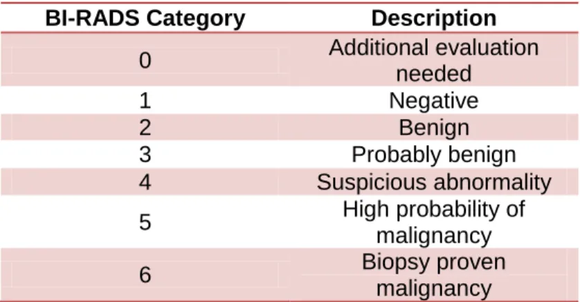
BI-28
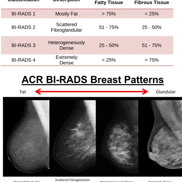
RADS classifies breast density into four categories based on the amount of fibrous tissue present in the breast. Table 2 shows the BI-RADS classifications for breast density and their respective fatty and fibrous tissue percentages. Figure 7 shows example 2D radiographs with each BI-RADS density classification. From the figure it can be seen as the breast density increases the image contrast decreases for 2D imaging modalities.
Table 2: BI-RADS breast density classifications. Data taken from Baker et al.35
Classification Description Percentage Fatty Tissue
Percentage Fibrous Tissue
BI-RADS 1 Mostly Fat > 75% < 25%
BI-RADS 2 Scattered
Fibroglandular 51 - 75% 25 - 50%
BI-RADS 3 Heterogeneously
Dense 25 - 50% 51 - 75%
BI-RADS 4 Extremely
Dense < 25% > 75%
Figure 7: Example 2D projection radiographs of breasts with each BI-RADS density classification. Moving from left to right the densities become more dense. This image is reprinted with permission from
29
3.2.3 Masses
There are two types of breast lesions typically associated with breast cancer, masses and MCs. Masses are abnormal groups of cells which could be benign (non-cancerous) or malignant (cancerous). There are a variety of lesions that can be found in the human breast. Table 3 lists a number of common lesions in the breast with their associated locations and disease.
Table 3: Typical lesions with their associated locations and disease. Data taken from Kopans.31 Benign - non-cancerous
Atypical - not associated with benign or malignant Malignant - cancerous
Name Location Disease
Duct ectasia Major ducts Benign
Large duct papilloma Major ducts Benign
Intraductal carcinoma extending from the terminal
ducts
Major ducts Malignant
Hyperplasia Minor and terminal ducts Atypical Peripheral duct papillomas Minor and terminal ducts Benign Ductal carcinoma Minor and terminal ducts Malignant
Cyst Lobule/Major ducts Benign
Fibroadenoma Lobule Benign
Adenosis Lobule Benign
Phylloides tumor Lobule Benign
Lobular carcinoma Lobule Malignant
Sarcoma Interlobular connective tissue Malignant