KIM_unc_0153D_13929.pdf

(1)

MORE EFFICIENT ESTIMATORS FOR CASE-COHORT

STUDIES WITH UNIVARIATE AND MULTIVARIATE

FAILURE TIMES

Soyoung Kim

A dissertation submitted to the faculty of the University of North Carolina at Chapel Hill in partial fulfillment of the requirements for the degree of Doctor of Philosophy in the Department of Biostatistics.

Chapel Hill 2013

Approved by: Dr. Jianwen Cai Dr. David Couper Dr. Ka He

(2)

c

(3)

Abstract

SOYOUNG KIM : More efficient estimators for case-cohort studies with univariate and multivariate failure times

(Under the direction of Dr. Jianwen Cai)

Case-cohort study design is generally used to reduce cost in large cohort studies when

the disease rate is low. The case-cohort design consists of a random sample of the entire

cohort, named subcohort, and all the subjects with the disease of interest. When the rate

of disease is not low or the number of cases are not small, the generalized case-cohort

study which selects subset of all cases is used. In this dissertation, we study more efficient

estimators of multiplicative hazards models and additive hazards models for the traditional

case-cohort study as well as the generalized case-cohort study.

We first study more efficient estimators for the traditional case-cohort studies with rare

diseases. When several diseases are of interest, several case-cohort studies are usually

con-ducted using the same subcohort. When these case-cohort data are analyzed, the common

practice is to analyze each disease separately ignoring data collected in subjects with the

other diseases. This is not an efficient use of the data. In this study, we propose more

efficient estimators by using all available information. We consider both joint analysis of

the multiple diseases and separate analysis for each disease. We propose an estimating

equation approach with a new weight function. We establish that the proposed estimator

is consistent and asymptotically normally distributed. Simulation studies show that the

proposed methods using all available information gain efficiency. For comparing the effect

of the exposure on different diseases, tests based on the joint analysis are more powerful

than those based on the separate analysis assuming independence. We apply our proposed

method to the data from the Busselton Health Study.

(4)

We also consider the additive hazards regression model for the stratified case-cohort

stud-ies. Additive hazards model is more appropriate when risk difference is of interest. Risk

difference is more relevant to public health because it translates directly into the number

of disease cases that would be avoided by eliminating a particular exposure. We propose

an estimating equation approach for parameter estimation in additive hazards regression

model by making full use of available information. Asymptotic properties of the proposed

estimators were developed and simulation studies were conducted. We apply our proposed

(5)

Acknowledgments

I would like to thank my dissertation advisor, Dr. Jianwen Cai for supporting me

during past three years. I have learned the lesson and gained the experience throughout my

dissertation research process. She has set an example of excellence as a researcher, mentor,

instructor, and role model.

I also would like to thank the committee members, Dr. David Couper, Dr. Ka He, Dr.

Wenbin Lu, Dr. Donglin Zeng, and Dr. Haibo Zhou for all of their guidance through this

(6)

List of Tables

3.1 Simulation result for a single disease outcome: β1=log(2) =0.693 . . . 47

3.2 Simulation result for multiple disease outcomes: [β₁, β₂] =[0.1,0.7] . . . . 48

3.3 Comparison between separate and joint analysis: β1=log 2, Pr(∆=1)=0.2 48

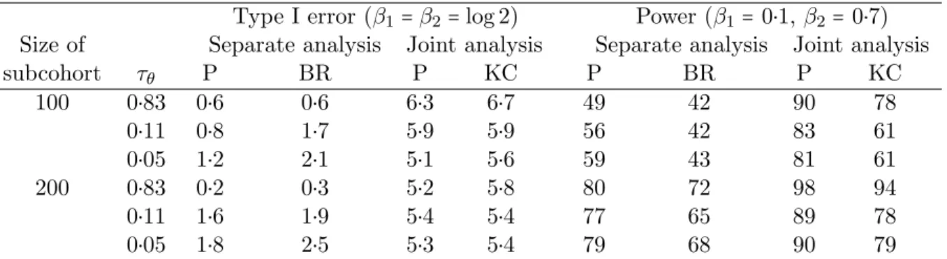
3.4 Type I error and power (%) in separate and joint analyses: Pr(∆=1)=0.2 . 49

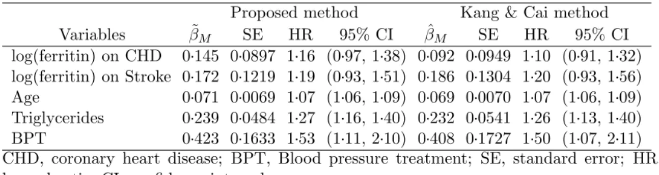
3.5 Analysis results for the Busselton Health Study . . . 51

4.1 Simulation result with a single disease outcome (K=1): β₁=log(2) =0.693 93

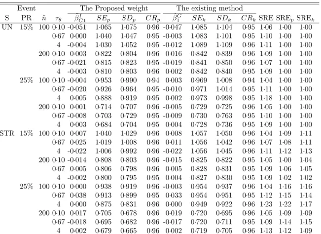
4.2 Simulation result with multiple disease outcomes (K =2): β=[0.1, 0.7] . . . 95

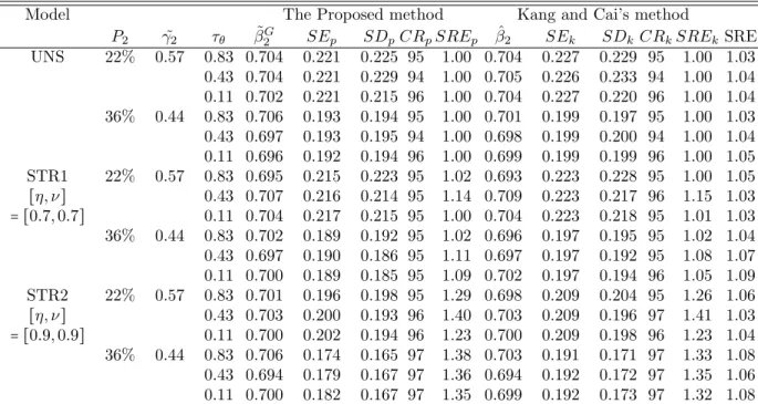
4.3 Type I error and power (%) in separate and joint analyses: [η, ν] = [0.7,0.7] 96

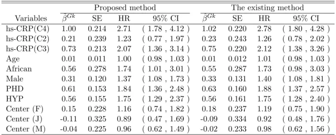
4.4 Results for the effect of hs-CRP from the ARIC Study . . . 98

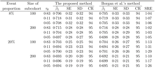
5.1 Simulation result for the traditional case-cohort study: K=1, β₁=0 . . . 131

5.2 Simulation result for the generalized case-cohort study: K=1,β₁ =0 . . . . 132

5.3 Simulation result for the traditional case-cohort study: K=2, β₀=0.3 . . . . 133

5.4 Simulation result for the generalized case-cohort study: K=2,β₀ =0.3 . . . 135

(9)

Chapter 1 Introduction

In large epidemiologic cohort studies, several thousands of subjects are usually followed

for many years and such studies can be expensive. Most of the cost and effort involve the

assembly of the covariate information for all cohort members. However, if the disease is rare,

much of the covariate information on disease free subjects is largely redundant [Prentice,

1986]. In order to reduce the high cost, Prentice [1986] proposed the case-cohort design.

Under the case-cohort study design, the covariate histories are collected only for subjects in

a randomly selected sample, named subcohort, from the entire cohort and all the cases (i.e.

the subjects with the event of interest). In this dissertation, we develop statistical methods

for case-cohort study design with univariate and multivariate failure time data.

One important advantage of the case-cohort study design is that the same subcohort can

be used for studying different diseases, whereas for other designs such as the nested

case-control design, new matching of cases and case-controls needs to be done for different diseases

[Wacholder et al., 1991; Langholz and Thomas, 1990].

For example, in the Busselton Health Study [Cullen, 1972] two case-cohort studies were

conducted. The purpose of this study is to investigate the effect of serum ferritin on

coro-nary heart disease and stroke, respectively. Serum ferritin was measured on a random

sample of the cohort as well as all subjects with coronary heart disease and/or stroke. The

existing methods do not use the covariate information collected on subjects with stroke

when studying the serum ferritin effect on coronary heart disease and vice versa. This is

(10)

exposure information is needed.

The case-cohort study design was originally proposed to reduce the cost in the cohort

study when the disease of interest is rare. Consequently, the traditional case-cohort sampling

involves all the cases (i.e. the subjects with the event of interest). In recent years, in order

to preserve the raw material collected in the study, case-cohort study design is also used

in situations when the disease is not rare. In such studies, it is not desirable to conduct

the traditional case-cohort studies which collect the expansive covariate information on all

cases. Sampling only a fraction of the cases is more practical [Breslow and Wellner, 2007;

Cai and Zeng, 2007; Kang and Cai, 2009]. Existing methods do not make the full use of

all available information about all diseases from the generalized case-cohort studies and a

correlate of the exposure available for all cohort members. It is desirable to develop new

statistical methods which use all available information.

There are two principal frameworks for modeling risks: the multiplicative and additive

risks model. Much work for the case-cohort studies were on multiplicative risks models

using proportional hazards models. However, the multiplicative risks model is not always

applicable in biomedical studies. Furthermore, the researchers could be interested in the

risk difference attributed to the exposure. The risk difference is more related to public

health since it translates directly into the number of disease cases that would be avoided by

eliminating a particular exposure [Kulich and Lin, 2000b]. Under such situation, the

addi-tive hazards model would be more appropriate. It will be important to develop statistical

methods for the additive hazards model using all available information from case-cohort or

generalized case-cohort studies.

(11)

Chapter 2 Literature review

In this chapter, we review the literature on statistical methods for both univariate and

multivariate survival data from cohort studies, case-cohort studies, and case-control studies.

The rest of this chapter is organized as follows. We review literature on statistical methods

in cohort studies for univariate failure time in section 2.1 and multivariate failure time

in section 2.2. In section 2.3, we review literature on statistical methods for case-cohort

studies.

2.1 Univariate failure time from cohort studies

In subsection 2.1.1, we first review the Cox proportional hazards model, the most popular

model for survival analysis with a single failure time. We review the literature on survival

analysis for additive hazards models from cohort studies in subsection 2.1.2.

2.1.1 The Cox proportional hazards model

The Cox proportional hazards model [Cox, 1972] is the most commonly used method

in survival analysis to examine the relationship between the effects of covariates and the

failure time. The Cox proportional hazards model specifies the hazard rate for failure time

T for a given covariate vector Z. Specifically, the Cox model is given by

λ{t∣Z} =λ₀(t)eβ T

(12)

whereλ0(t) is an unspecified baseline hazard function and β₀ is ap-dimensional fixed and

unknown parameter vector.

LetTi be the failure time, Ci denote the potential censoring time, andXi=min(T_i, C_i)

denote the observed time for subject i. Let Yi(t) =I(X_i ≥t) be an at risk indicator and

∆i =I(T_i ≤C_i) be failure indicator where I(.) is the indicator function for subject i. Let Ni(t) = I(X_i ≤ t,∆_i = 1) denote the observed counting process for failure for subject i.

Suppose that there are nindependent subjects and τ denotes the end of study time. The partial likelihood score function introduced by Cox [1975] is given by

U1(β) =

n

∑

i=1

{Z_i(X_i) −S (1)

(β, X_i) S(0)₍_{β, X}

i) }∆_i,

or equivalently using counting process form

U2(β) =

n

∑

i=1 ∫

τ

0 Zi

(u)dN_i(u_{) − ∫}

τ

0 S(1)

(β, u) S(0)₍_{β, u}₎d

¯ Ni(u),

where

¯ Ni(t) =

n

∑

i=1

Ni(t), S(0)(β, t) =n−1

n

∑

i=1

Yi(t)eβ

′_Z_i₍_t₎ , S(1)

(β, t) =n−1

n

∑

i=1

Yi(t)Z_i(t)eβ

′_Z_i₍_t₎ .

The regression parameter β can be estimated by solving the score equation U2(β) =0.

We denote the solution by ˆβ. Under some regularity conditions, ˆβ has been shown to be consistent and follow a normal distribution with meanβ0 and covariance matrix Σ given by

Σ_{= ∫}

τ

0 v

(β₀, t)s(0)(β₀, t)λ₀(t)dt,

wherev(β₀, t) =s(2)(β₀, t)/s(0)(β₀, t) − {s(1)(β₀, t)/s(0)(β₀, t)}⊗2,s(d)(β₀, t) =

E[S(d)(β₀, t)] for d=0,1,2, and S(2)(β, t) =n−1∑n_i₌₁Yi(t)Z_i(t)⊗2eβ′Zi(t). The asymptotic

variance Σ can be estimated by_Σ̂_{= −{}_∂U

2(β)/∂β∣_β

(13)

2.1.2 Additive hazards model

Another framework commonly used for regression with censored failure time is the

addi-tive hazards model. Much work has been conducted under the assumption of multiplicaaddi-tive

hazards models. However, epidemiologists often are interested in the risk difference. Risk

difference is another measure of association. It is very relevant to public health decisions,

because it translates directly to the expected number of disease cases that would be

pre-vented in the population by removing a certain exposure [Kulich and Lin, 2000b]. When

the risk difference is of interest, the additive hazards model is very useful.

The additive hazards model takes the following form:

λa(t;Z) =λ_a₀(t) +β_a′₀Z(t), (2.2)

where Z(.) is ap-vector of possibly time-varying covariates, β_a₀ is a p-vector of regression

parameters, and λa0(t) is an unspecified baseline hazard function. The regression

param-eter of the additive hazards model represents the risk difference for one unit change in

the covariate while adjusting for the other covariates in the model. Lin and Ying [1994]

proposed estimators under model (2.2) and studied the asymptotic properties of the

esti-mators. Mimicking the partial likelihood score function for the proportional hazards model,

the estimating function to estimate βa0 in (2.2) is given by

Ua(β) =

n

∑

i=1 ∫

τ

0

{Z_i(t) −Z¯_a(t)} {dN_i(t) −Y_i(t)β_a′Z_i(t)dt},

where ¯Za(t) = ∑n_j=1Yj(t)Zj(t)/ ∑

n

j=1Yj(t). The estimator ˆβa is defined as the solution to U(β) =0 and takes the explicit form

ˆ βa= [

n

∑

i=1 ∫

τ

0 Yi

(t){Z_i(t) −Z¯_a(t)}⊗2dt] −1

[

n

∑

i=1 ∫

τ

0

{Z_i(t) −Z¯_a(t)}dN_i(t)].

Under some regularity conditions, Lin and Ying [1994] showed the random vector

n−1/2

(14)

with a covariance matrix which can be consistently estimated byA−1_BA−1_{, where}

A=n−1

n

∑

i=1 ∫

τ

0 Yi

(t) {Z_i(t) −Z¯_a(t)} ⊗2

dt and B=n−1

n

∑

i=1 ∫

τ

0

{Z_i(t) −Z¯_a(t)} ⊗2

dNi(t).

Lin and Ying [1994] also proposed the estimator for the baseline cumulative hazard function:

ˆ

Λa0(βˆ_a, t_{) = ∫}

t

0

∑n_i₌₁{dN_i(u) −Y_i(u)βˆ_a′Z_i(u)du} ∑n_j=1Yj(t)

.

They also showed that n1/2

{Λˆ_a₀(β, .ˆ ) −Λ₀(.)} converges weakly to a zero-mean Gaussian

process whose covariance function at (t, s)(t≥s) can be consistently estimated by

∫

s

0

n∑n_i₌₁dNi(u) {∑nj=1Yj(u)}

2 +C

′

(t)A−1BA−1C(s) −C′(t)A−1D(s) −C′(s)A−1D(t),

whereC(t_{) = ∫}₀tZ¯_a(u)duand D(t_{) = ∫}₀t∑ n

i₌1{Zi(u)−Z¯a(u)}dNi(u) ∑nj₌1Yj(u) .

2.2 Multivariate failure time from cohort studies

In section 2.2, we review the literature on survival analysis for multivariate failure time

data. Several approaches dealing with multiple failure times or recurrent event data have

been proposed. We review literature on statistical methods for multiplicative hazards

mod-els in subsection 2.2.1 and additive hazards modmod-els in subsection 2.2.2.

2.2.1 Multiplicative risk models

There are in general two types of commonly used models dealing with correlated failure

times: 1) marginal models, 2) frailty models. The marginal model approach does not

specify the form of the dependence among correlated failure times while the frailty model

approach formulates the exact nature of dependence among correlated failure times through

(15)

Marginal models

Several authors have studied marginal models. Wei et al. [1989] proposed semiparametric

methods for each marginal distribution of failure times with Cox-type proportional hazards

form.

Let Zik(t) = (Z_i₁_k(t), . . . , Z_ipk(t))′ be the covariate vector for the ith subject and the kth failure type and βk= (β₁_k, . . . , β_pk)′be the failure-specific regression parameter. Under

the failure-specific model, the hazard function for the ith subject and the kth failure type is given by

λk{t∣Z_ik(t)} =λ₀_k(t)eβkZik(t), (2.3)

whereλ0k(t) is an unspecified baseline hazard function fork=1, . . . , K.

The kth failure-specific partial likelihood function [Cox, 1972, 1975] is

Lk(β_k) =

n

∏

i=1 [

exp{β_k′Z_ik(X_ik)} ∑_l_∈R

k(Xik)exp{β ′

kZlk(Xik)}

]

∆ik ,

whereR_k(t) = {l∶X_lk≥t}is the set of subjects at risk just prior to timetwith respect to the kth type of failure. The maximum partial likelihood estimator ˆβk is defined as the solution

to the partial likelihood equation ∂logLk(β_k)/∂β_k = 0 and they are generally correlated.

Under some regularity conditions, it is shown that ˆβk is a consistent estimator for βk and

n1/2 (βˆ′

1−β′1, . . . ,βˆ′K−βK′ )converges in distribution to a zero-mean normal random vector

with covariance matrix Qwhere

Q= ⎡ ⎢ ⎢ ⎢ ⎢ ⎢ ⎢ ⎢ ⎢ ⎢ ⎣

H11(β₁, β₁) ⋯ H₁_K(β₁, β_K)

⋮ ⋮

(16)

with

Hkl(β_k, β_l) =A_k−1(β_k)E{w₁_k(β_k)w₁_l(β_l)′}A−_l1(β_l), Ak(β_k_{) = ∫}

τ

0 vk

(β_k, t)s(_k0)(β_k, t)λ₀_k(t)dt, vk(β, t) =s(2)

k (β, t)/s

(0)

k (β, t) − {s

(1)

k (βk, t)/s

(0)

k (βk, t)}

⊗2 , s(_kd)(β, t) =E[Y₁_k(t)Z₁_k(t)⊗dexp{β′Z₁_k(t)}],

wik(β_k_{) = ∫} ∞

0

{Z_ik(t) −s(1)

k (βk, t)/s

(0)

k (βk, t)}dMik(t), and

Mik(t) =N_ik(t_{) − ∫}

t

0 Yik

(t)λ_ik(u)du.

Spiekerman and Lin [1998] and Clegg et al. [1999] extended the models proposed by

Wei et al. [1989] to formulate the general form by allowing for exchangeable failure time

of each distinct failure type in the cluster. Suppose that there are J clusters, K distinct failure types, each of which consists of L exchangeable failure times. Let Tjkl denote the

failure time and Cjkl the censoring time, and Xjkl=min(T_jkl, C_jkl) the observed time for

component l of disease k in cluster j. Let Yjkl(t) = I(X_jkl ≥ t) be an at risk indicator,

∆jkl=I(T_jkl≤C_jkl) be failure indicator whereI(.)is the indicator function and N_jkl(t) = I(X_jkl≤t,∆_jkl=1)be the observed counting process for failure for component lof disease k in cluster j. Specifically, the following model for the lth component of the kth type of failure is considered:

λkl{t∣Z_kl(t)} =λ₀_k(t)eβ T

0Zkl(t) ,

whereλ0k(t)(k=1, . . . , K)are unspecified baseline hazard functions.

The pseudo-partial score function is given by

USL(β) =

J

∑

j=1

K

∑

k=1

L

∑

l=1 ∫

τ

0

{Z_jkl(u) −

S_k(1)(β, u) S(0)

k (β, u)

}dN_jkl(u),

where Zjkl is the covariate vector for thelth component of thekth failure type in thejth

cluster and S(d)

k (β, t) =J

−1

∑J_j=1∑

L

l=1Yjkl(t)Zjkl(t)

(17)

The maximum pseudo-partial-likelihood estimator ˆβSL for β0 is defined as the solu-tion to USL(β) = 0 and n1/2(βˆ_SL−β₀) is shown to converge weakly to a p-variate

nor-mal vector with mean 0 and covariance matrix Ω = A−1B_SLA−1 where A = ∑K_k=1Ak and BSL = E_[∫₀τ{Z_jkl(u) − S

(1)

k (β0,u)

S(_k0)(β0,u)

}dM_jkl(u)]⊗2. In addition, Spiekerman and Lin [1998]

showed the uniform convergence and joint weak convergence of the Aalen-Breslow type

estimators for the cumulative baseline hazard functions ˆΛ0k(t, β)where

ˆ

Λ0k(t,βˆ_{) = ∫}

t

0

dN.k.(u) nS_k(0)(β, uˆ )

.

Frailty models

Marginal model approaches are appropriate when the main interest is to estimate the

effects of risk factors while the correlation among failure times is considered as a nuisance.

However, when the correlation among failure times is of interest, an alternative approach

is needed. Frailty models have been proposed under such situation. Frailty model specifies

the intra-subject correlation explicitly through an unobservable random variable (frailty).

Specifically, the failure times given the frailty are assumed independent and the conditional

hazard given the frailtyWi is assumed to follow the following model:

λik(t∣W_i) =W_iλ₀(t)exp{βT₀Z_ik(t)},

whereWi,i=1, . . . , n, are assumed to be independent and follow a probability distribution

is often assumed for the frailty distribution. Other distributions such as the positive stable

distribution, the inverse Gaussian distribution, or the log-normal distribution have also been

proposed.

Frailty models have been studied by many authors. In approaches for nonparametric

maximum likelihood, Klein [1992] proposed the estimation of the frailty by using an EM

algorithm based on a partial likelihood. As an alternative of a partial likelihood, a

penal-ized likelihood procedure is used by Therneau and Grambsch [2000] who showed an exact

(18)

Ripatti and Palmgren [2000] generalized the results of Therneau and Grambsch [2000] by

as-suming the frailties from a log-normal distribution and thus they got a flexible specification

of variance components which can explain negative dependencies.

2.2.2 Additive risk models

The previous subsection discussed multiplicative hazards models. In this subsection, we

will review additive hazards models with multivariate failure time data from cohort studies.

When all the failure times are independent, several authors have studied additive hazards

models from cohort studies. Martinussen and Scheike [2002] and Lin et al. [1998] has applied

the additive hazards model to interval censored data. Moreover, the additive hazards model

has been applied to measurement error problems by Kulich and Lin [2000b], to frailty models

by Lin and Ying [1997], and to cumulative incidence rates by Shen and Cheng [1999].

For correlated or clustered data, marginal additive hazards models are proposed by Yin

and Cai [2004]. They proposed the additive hazards model

Λjki(t;Z_jki) =λ₀_k(t) +β₀′_kZ_ikl(t),

where Zjki(t) is a possibly time-varying covariate vector for failure type k of subject i in

cluster j. An estimating function forβ0k is

U_kA(β) =

J

∑

j=1

n

∑

i=1 ∫

τ

0

{Z_jki(t) −Z¯_kA(t)} {dN_jki(t) −Y_jki(t)β′Z_jki(t)dt},

where ¯Z_kA(t) =

∑J_j₌₁∑n_i₌₁Yjki(t)Zjki(t)

∑Jj₌1∑ni₌1Yjki(t) . The estimator ˆβ

A

k is defined as the solution toUkA(β) =

0, which is given by

ˆ β_kA=

⎡ ⎢ ⎢ ⎢ ⎢ ⎣

J

∑

j=1

n

∑

i=1 ∫

τ

0 Yjki

(t){Z_jki(t) −Z¯_kA(t)}⊗2dt ⎤ ⎥ ⎥ ⎥ ⎥ ⎦

−1_⎡ ⎢ ⎢ ⎢ ⎢ ⎣

J

∑

j=1

n

∑

i=1 ∫

τ

0

{Z_jki(t) −Z¯_kA(t)}dN_jki(t) ⎤ ⎥ ⎥ ⎥ ⎥ ⎦ .

Under some regularity conditions, n1/2

(βˆ₁A′−β₀₁′ , . . . ,βˆA_K′−β₀′_K)′ was shown to converge in

(19)

vectorD_jkA(β′₀_j, β₀′_k) =A−_j1E[U₁A_j(β₀_j)U₁A_k(β₀_k)]A_j−1 whereA_j =E[∑L_l₌₁∫

τ

0 Y1jl(t){Z₁_jl(t) −

¯

Zj(t)}⊗2dt]. Under the working independence assumption, the baseline cumulative hazard

function for failure typek can be estimated by

ˆ

ΛA₀_k(t; ˆβ_k_{) = ∫}

τ

0

∑J_j=1∑

n

i=1{dNjki(u) −Yjki(u)βˆ

A′

k Zjki(u)du} ∑J_j₌₁∑n_i₌₁Yjki(u)

.

Under some regularity conditions, as n → ∞, n1/2[{ΛˆA₀₁(t) −Λ01(t)}, . . . ,{ΛˆA₀_K(t) −

Λ0K(t)}] was shown to converge weakly to a zero-mean Gaussian random field. For a

specific subject with the covariate vectorZ0(t), the cumulative hazard function can be

es-timated by ˆΛA(t; ˆβ_kA, Z₀) = ΛˆA₀_k(t; ˆβ_kA_{) + ∫}₀tβˆ_kA′Z₀(u)du. To ensure monotonicity, a minor

modification was made, i.e. ˆΛ∗

0k(t) =maxs≤tΛˆ

A

0k(s) for k=1, . . . , K. By similar arguments

as in Lin and Ying [1994], it can be shown that ˆΛ∗

0k(t) and ˆΛA0k(t) are asymptotically

equivalent.

Pipper and Martinusse [2004] also considered marginal additive hazards models for

clus-tered data. By using Lin and Ying [1994]’s estimators, they provided estimating equations

for the regression parameters and association parameters for marginal additive hazards

models. Further, Yin [2007] developed a test for checking the additive structure using

clus-tered data. By relaxing the linear assumption about covariate effects, Zeng and Cai [2010]

proposed a general class of additive transformation risk models for clustered failure time

data.

2.3 Case-cohort studies

2.3.1 Case-cohort studies vs nested case-control studies

In large epidemiologic cohort studies, several thousands of subjects are followed and

thus such studies can be expensive. To reduce the cost in large cohort studies, several study

designs have been proposed. Among different sampling schemes, nested case-control study

design and case-cohort study design are widely used when the disease rate is low. In this

subsection, we will review the literature on nested case-control study design and case-cohort

(20)

Thomas [1977] originally suggested nested cacontrol study design which involves

se-lection of a number of controls from those at risk at the failure time of each case. Prentice

and Breslow [1978] further developed the conceptual foundations of the nested case-control

design by deriving the conditional likelihood. However, there are some limitations in the

nested case-control studies: inefficiency for the alignment of each selected control subject

to its matched case and a strict application which involves the selection of a new set of

controls for each distinct disease category.

To address the problems, case-cohort study design was proposed by Prentice [1986] as

an alternative to the nested case-control study design. Case-cohort study design involves

selection of a random sample, named subcohort, and all cases. The subcohort constitutes

the comparison set of cases occurring at a range of failure times. The subcohort also provides

a basis for covariate monitoring during the course of cohort follow-up [Prentice, 1986].

Langholz and Thomas [1990] compared case-cohort studies with nested case-control

studies. They showed that the nested case-control approach is better than the case-cohort

study if there is moderate random censoring or staggered entry. It also has been shown

that case-cohort study design for a single disease outcome has higher efficiency than nested

case-control study design; however, the difference is very small. Compared to the nested

case-control studies, a major advantage of the case-cohort design is the ability to study

several disease outcomes using the same subcohort.

We will review the literature for case-cohort studies with univariate failure time in

subsection 2.3.2 and multivariate failure time in subsection 2.3.3.

2.3.2 Univariate failure time

Prentice [1986] proposed a case-cohort design and established asymptotic properties of

their proposed estimators. He considered a relative risk regression model [Cox, 1972]:

λ{t∣Z(u),0≤u<t} =λ₀(t)r{β′₀Z_i(t)}, (2.4)

(21)

λ0(t) is a baseline hazard function.

Prentice [1986] proposed the pseudolikelihood function for estimation of the relative risk

parameterβ0 in case-cohort studies given by

̃ L(β) =

n

∏

i=1 ⎛ ⎜ ⎝

rii/ ∑

l∈R(˜ ti) rli

⎞ ⎟ ⎠

∆i

where rli = Y_l(t_i)r{β₀′Z_l(t_i)}, ˜R(t_i) = F(t) ∪C˜, F(t) = {i∣N_i(t) ≠ N_i(t−)}, and ˜C is a

random subcohort.

The maximum pseudolikelihood estimator ˜βCC is defined as a solution to UCC(β˜) = 0

where

UCC(β) = ∂log ̃ L(β)

∂β =

n

∑

i=1

Ui(β) =

n

∑

i=1 ∆i

⎛ ⎜ ⎝

cii− ∑

l∈R(˜ ti)

bli/ ∑

l∈R(˜ ti) rli

⎞ ⎟ ⎠ ,

bli = Y_l(t_i)Z_l(t_i)r′{βTZ_l(t_i)}, c_li = b_lir−1{βTZ_l(t_i)}, and r′(u) = dr(u)/du. Under some

regularity conditions, Prentice [1986] reasoned thatn−1/2_U

CC(β)converge weakly to a

nor-mal variate with mean zero and variance matrix A and that n1/2

(β˜_CC−β₀) converges in

distribution to a normal variate with mean zero and variance matrix S =Ω−1AΩ−1 which

can be estimated by nI(β˜)−1V˜(β˜)I(β˜)−1 where

I(β) = −

∂2log_L̃₍_β₎ ∂β∂βT ,

˜

V(β) =

n

∑

j=1

∆j{v_jj+2δ(t_j) ∑ {k∣tk<tj}

∆kvkj},

vkj = − ∑ (

Bk+b_jk−b_ik Rk+r_jk−r_ik )

′ (c_ij −

Bj

Rj

)r_ijR_j−1,

Rj = ∑

l∈R(˜ tj)

rlj, Bj= ∑

l∈R(˜ tj)

blj, δ(t) =0 if C˜=R(˜ t) and 1 otherwise.

An estimator of the baseline cumulative failure rate function Λ0(t_{) = ∫}₀tλ₀(u)duis

ˆ

Λ0(t) =nn˜ −1_∫

t

0

[

n

∑

i=1

(22)

where ¯N(t) = ∑n_i=1Ni(t).

Self and Prentice [1988] proposed a slightly different estimator from Prentice [1986].

While the “comparison risk set” of Self and Prentice [1988] at timet included only all sub-cohort members at risk at timet, Prentice [1986] added any subjects out of subcohort but who were observed to fail at time t. Self and Prentice [1988] established asymptotic dis-tribution theory for the pseudolikelihood estimators along with that for the corresponding

cumulative failure rate estimators by using a combination of martingale and finite

pop-ulation convergence results. Specifically, they considered the maximum pseudolikelihood

estimator ˜βSP, defined as a solution to∂logL(β˜)/∂β=0, where

log_L̃₍_β_{) =}

n

∑

i=1 ∫

τ

0 logr

{β′Z_i(t)}dN_i(t_{) − ∫}

τ

0 log[ ∑

i∈C˜

Yl(t)r{β′Z_i(t)}]dN¯(t),

and ˜C is a random subcohort of size ˜n. They also considered a natural estimator of the cumulative baseline hazard function which is given by

˜

ΛSP(t) =˜nn−1_∫

t

0 [ ∑

i∈C˜

Yi(u)r{β˜_SP′ Z_i(u)}]−1dN¯(u).

Under some regularity conditions, they showed that ˜βSP is a consistent estimator ofβ0 and n−1/2_U˜

(β₀)converges in distribution to zero mean Gaussian process with covariance matrix

Σ(β₀) +A(β₀) where Σ(β) = −lim_n_→∞n−1∂2logL̃(β)/∂β2 is the variation associated with

the cohort and A(β) corresponds to the variation introduced by sampling the subcohort.

Therefore, n−1/2

(β˜_SP −β₀)was shown to converge in distribution to a zero-mean Gaussian

random variable with covariance matrix Σ−1

(β₀) +Σ−1(β₀)A(β₀)Σ−1(β₀) by Taylor series

expansions. Moreover,n−1/2

(β˜_SP−β₀)and n−1/2(Λ˜_SP−Λ₀)were shown to converge weakly

and jointly to Gaussian random variables with mean zero. They also proposed the estimator

of the limiting covariance matrix betweenn−1/2

{Λ˜_SP(u)−Λ₀(u)}andn−1/2{Λ˜_SP(t)−Λ₀(t)}.

Self and Prentice [1988] showed that Prentice [1986]’s estimator ˜β and their estimator ˜

βSP are asymptotically equivalent by showing that an individual’s contributions to S(1)

(23)

is somewhat different from Self and Prentice [1988]’s one, two estimators converge to the

same form asymptotically.

Alternative variance estimators which can be computed easily using the existing software

are proposed since the variance estimators by Prentice [1986] and Self and Prentice [1988]

are complicated. Wacholder et al. [1989] developed bootstrap variance estimates. Barlow

[1994] proposed a robust estimator of the variance. By using time-varying weights, he

proposed a pseudolikelihood function which are different from those of Prentice [1986] and

Self and Prentice [1988]. The weight wi(t)of subject iat timet is defined as

wi(t) = ⎧ ⎪ ⎪ ⎪ ⎪ ⎪ ⎪ ⎪ ⎪ ⎨ ⎪ ⎪ ⎪ ⎪ ⎪ ⎪ ⎪ ⎪ ⎩

1 ifdNi(t) =1

m(t)/m˜(t) ifdN_i(t) =0 andi∈C˜

0 ifdNi(t) =0 andi/∈C.˜ ⎫ ⎪ ⎪ ⎪ ⎪ ⎪ ⎪ ⎪ ⎪ ⎬ ⎪ ⎪ ⎪ ⎪ ⎪ ⎪ ⎪ ⎪ ⎭

wherem(t)is the number of disease-free individuals in the cohort at risk at timetand ˜m(t)

is the number of disease-free individuals in subcohort at risk at time t. The conditional probability of failure at failure time tj is given by

pi(t_j) =

Yi(t_j)w_i(t_j)r_i(t_j) ∑n_k₌₁Yk(t_j)w_k(t_j)r_k(t_j)

,

where ri(t) = exp{β₀TZ_i(t)}. Prentice [1986]’s likelihood used an indicator function as a

weight, i.e., wi(t) = 1 if dN_i(t) = 1 or i∈ C˜, otherwise the weight is zero. Whereas Self

and Prentice [1988]’s likelihood used a denominator summed over subcohort members only,

Barlow [1994]’s pseudolikelihood preserved the correct expectation for the denominator at

each failure time.

The estimator ˆβBproposed by Barlow [1994] is defined as the solution to the estimating

equation defined by the derivative of the logarithm of the pseudolikelihood∑_t∑_idNi(t)

log(p_i(t)). The robust variance estimator using infinitesimal jackknife estimator is

ˆ

V ar(βˆ_B) =I−1(βˆ_B)Vˆ(βˆ_B)I−1(βˆ_B) = 1

(24)

where ˆei=βˆ−β−ˆ _iand ˆβ−_i is an estimate ofβ without observationi. Barlow [1994] proposed

to estimate ˆei by I−1(βˆ)ˆc_i(τ) where I(βˆ_B) = ∑t∑_ipˆi(t)[z_i(t) −Eˆ(t)][z_i(t) −Eˆ(t)]′ is the

information matrix, ˆE(t) = ∑n_k=1pˆi(t)Zi(t) is the estimator for the conditional expectation of the covariate at time t, and ˆci(τ_{) = ∫}₀τY_i(t)[dN_i(t) −pˆ_i(t)][z_i(t) −Eˆ(t)]dN¯(t) is the

estimated influence of an individual observation on the overall score for subjectiat timeτ. Stratified case-cohort studies were discussed in Prentice [1986]. Borgan et al. [2000]

developed methods for analysis of such exposure stratified case-cohort samples. Suppose

that the baseline data are available for the full cohort and can be partitioned intoQstrata. A stratified relative risk regression model is considered:

λq{t∣Z(t)} =λ₀_q(t)r{β_qTZ(t)}, q=1, . . . , Q.

A pseudolikelihood function for β over strata is

˜

Lq(β) = ∏

tj ⎛ ⎝

exp{β′Z_i_j(t_j)}w_i_j(t_j) ∑_k_∈R(˜ tj)Yk(tj)exp{β

′_Z

k(t_j)}w_k(t_j) ⎞ ⎠ ,

where tj is failure time, ˜R(t_j) is case-cohort set, and w_i_j(t_j) is weight for the case i_j at

timetj. They proposed three types of estimators for the stratified case-cohort design:

I ∶ R(˜ t_j) =C, w˜ _k(t_j) =n_s₍_k₎/m_s₍_k), II ∶ R(˜ t_j) =C˜∪F, w_k(t_j) =n0_s

(k)/m 0

s(k) ifk∈C˜/F, wk(tj) =1 if k∈F, III ∶ w_k(t_j) =n_s₍_k₎/m_s₍_k₎,R(˜ t_j) =C˜ ifi_j ∈C,˜ R(˜ t_j) =C˜∪i_j/{J_s₍_i

j)} ifij /∈C,˜ where ˜C is the subcohort set,F is a set of all cases,nl and ml are the number of subjects

in the cohort and subcohort in stratuml, respectively,n0_l and m0_l are the number of cases in the cohort and subcohort in stratuml, respectively, and s(k)is the sampling stratum of

individualk. If the case occurs outside the subcohort, subcohort memberJs(ij)swaps place with the case so that the caseij is inside ˜R(t_j) while the “swapper”J_s₍_i

j) is removed from this set. They showed that all of the proposed analysis methods were more efficient than

(25)

results of Borgan et al. [2000] by using weighted likelihood estimation in two-phase stratified

sample.

Chen [2001b] proposed a unified approach which includes 1) nested case-control

sam-pling, 2) case-cohort samsam-pling, and 3) classical case-control designs and allow the presence

of staggered entry. The estimating equation to cover three samplings is given by

UCh(β) =

n

∑

i=1 ∫

τ

0

[Z_i(t) −

∑n_j₌₁wijZj(t)exp{β′Z_j(t)}Y_j(t) ∑n_j₌₁wijexp{β′Z_j(t)}Y_j(t)

]dN_i(t),

where wij is a weight function for the respective design. They also developed the weight

function based on estimating each missing covariate by a local average. Samuelsen et al.

[2007] extended the class of designs proposed by Chen [2001b] to accommodate stratified

designs.

All work that we discussed in this subsection so far was about proportional hazards

mod-els for case-cohort studies. Other type of modmod-els have also been studied. The accelerated

failure time model and the proportional odds regression model for case-cohort are proposed

[Kong and Cai, 2009; Chen, 2001a]. Kulich and Lin [2000a] applied additive hazards

mod-els to case-cohort studies. The model they considered is in the same form as (2.2). The

subcohort can be selected by Bernoulli sampling with arbitrary selection probabilities or

by stratified simple random sampling. Using Bernoulli sampling, they proposed a weighted

estimating function:

UH(β) =

n

∑

i=1 ρi∫

τ

0

{Z_i(t) −Z¯_H(t)} {dN_i(t) −Y_i(t)βTZ_i(t)dt},

where ¯ZH(t) = ∑ n

j=1ρjYj(t)Zj(t)

∑n_j₌₁ρjYj(t) and the weight function ρi has the following form: ρi = ∆i+ (1−∆_i)ξ_iαˆ−1, and ˆα= ∑n_i=1ξi(1−∆i)/ ∑

n

i=1(1−∆i). The estimator ˆβH is defined as a solution to UH(β) =0. An estimator for the cumulative baseline hazard function Λ0(t) is

ˆ

Λ0H(t_{) = ∫}

τ

0

∑n_i₌₁dNi(u) ∑n_j=1ρjYj(u)

− ∫

τ

0 ˆ

βHZ¯H(u)du.

Under some regularity conditions, n1/2

(26)

to a zero-mean normal random vector with covariance matrix D−1

A(ΣA+Σ_H)D_A−1, where DA=E_[∫₀τ{Z₁(t)−e(t)}⊗2Y₁(t)dt], Σ_A(β) =E_[∫₀τ{Z₁(t)−e(t)}⊗2dN₁(t)], Σ_H(β) =E{(1−

˜

α)α˜−1(1−∆1_)[∫₀τ{Z₁(t) −e(t)}dM₁(t)]⊗2}, e(t) = E{Z₁(t)Y₁(t)}/E{Y₁(t)}, and M_i(t) = Ni(t_{) − ∫}₀tY_i(s)sΛ0(s_{) − ∫}₀tβ₀TZ_i(s)Y_i(s)ds. They also showed that n1/2(Λ0ˆ _H(t) −Λ0_H(t))

converges weakly on [0, τ] to a zero-mean Gaussian process whose covariance function at (s, t) is

hT(s)D_A−1(Σ_A+Σ_H)D−_A1h(t) +R₁(s, t) −hT(s)D−_A1R₂(t) −hT(t)D−_A1R₂(s),

whereR1(s, t) =E[{∆₁+(1−∆₁)/α˜_{} ∫}₀sπ−₀1(u)dM₁(u_{) ∫}₀tπ−₀1(v)dM₁(v)],R₂(t) =E_[∫₀t{Z₁(u)− e(u)}π₀−1(u)dN₁(u)],h(t_{) = ∫}₀te(u)du, and π₀(u) =Pr(X₁≥t).

2.3.3 Multivariate failure time

Clustered failure time and multiple outcomes have been studied for the case-cohort

design. In this subsection, we will review the related literature.

Lu and Shih [2006] considered the clustered failure time data. Conventional case-cohort

studies for univariate failure time data cannot be directly applied to clustered failure time

data since failure times within a cluster are correlated. Lu and Shih [2006] considered

marginal proportional hazards model (2.4). Suppose there areJ independent clusters, and each cluster contains n correlated subjects. The estimating function proposed by Lu and Shih [2006] is given by

ULS(β) =

J

∑

j=1

n

∑

i=1 ∫

τ

0

[Z_ji(t) −E_LS(β, t)dN_ji(t)],

whereELS(β, t) =S_LS(1)(β, t)/S_LS(0)(β, t),S_LS(d)(β, t) =J−1∑J_j ∑_in₌₁HjHjiYji(t)e{β T_Z

ji(t)} ×Z_ji(t)⊗d,H_j indicates whether or not clusterjis selected into the subcohort, andH_jiis the

indicator for subject(j, i)being sampled as a potential individual in the subcohort. ˜β_LS can

be estimated by solvingULS(β) =0. Under some regularity conditions, ˜β_LS was shown to be

(27)

normal distribution with mean zero and with covariance matrix A−1

LS(β0)ΩLS(β₀)A−_LS1(β₀)

where ΩLS(β)consists of the variations associated with the cohort and subcohort sampling

and ALS(β) = −lim_J_→∞∂U_LS(β)/∂β.

Zhang et al. [2011] extended Lu and Shih [2006]’s method by proposing Bernoulli

sam-pling and using different risk sets. Since information on all failures in the full cohort is

available, failures outside the subcohort can also contribute to the risk set for independent

subjects. Thus, they constructed the risk sets using the information in the subcohort as

well as the information collected on future deaths whereas Lu and Shih [2006] used only

subcohort subjects to construct the risk set.

Kang and Cai [2009] considered case-cohort studies with multiple disease outcomes. The

marginal hazards function [Cox, 1972] is assumed to follow the model:

λik{t∣Z_ik(t)} =Y_ik(t)λ₀_k(t)eβ T

0Zik(t) ,

whereλ0k(t)is an unspecified baseline hazard function for disease outcomek. The

pseudo-partial likelihood score equation proposed by Kang and Cai [2009] is given by

̂

UKC(β) =

n

∑

i=1

K

∑

k=1 ∫

τ

0

{Z_ik(t) − ̂ S(1)

k (β, t)

̂

S_k(0)(β, t)

}dN_ik(t),

where_Ŝ(d)

k (β, t) =n

−1

∑n_i=1ρik(t)Yik(t)Z ⊗d

ik (t)e

βTZik(t)_for_d_{= 0,1 and 2,}_ρ

ik(t) =∆_ik+ (1−

∆ik)ξ_iαˆ_k−1(t), and ˆα_k(t) = ∑n_i=1(1−∆ik)ξiYik(t)/{∑

n

i=1(1−∆ik)Yik(t)}. Moreover, Kang and Cai [2009] proposed a weighted estimating equation approach for estimating the parameters

in the marginal hazards regression models for the multivariate failure time data from the

generalized case-cohort study with multiple disease outcomes. The weighted estimating

function follows as

̃

UKC(β) =

n

∑

i=1

K

∑

k=1 ∫

τ

0 wik

(t){Z_ik(t) − ̃ S(1)

k (β, t)

̃ S(0)

k (β, t)

}dN_ik(t),

where _S̃(d)

k (β, t) = n

−1

∑n_i=1wik(t)Yik(t)Z ⊗d

ik (t)e βT_Z

ik(t) _for _d _{= 0,1 and 2 ,} _w

ik(t) = (1−

(28)

ξi)Y_ik(t)},η_ik is an indicator for subject ioutside the subcohort by random sampling. The

estimator ˜βKC is defined as solution to the equations ŨKC(β) =0. A Breslow-Aalen-type

estimator of the baseline cumulative hazard function is ˜Λ0k(β˜_KC, t), where

˜

Λ0k(β, t_{) = ∫}

t

0

∑n_i₌₁wik(u)dN_ik(u) nS˜(0)

k (β, u)

Under some regularity conditions, they showed that ˜βKC is a consistent estimator ofβ0 and n1/2

(β˜_KC−β₀) is asymptotically normally distributed with mean zero and with variance

matrix in the form

ΣKC(β₀) =A(β₀)−1{Q(β₀) +

1−α

α V1(β0) + (1−α)

K

∑

k=1

pr(∆₁_k=1)(

1−q_k qk

)V₂_k(β₀)}A(β₀)−1,

where

A(β) =

K

∑

k=1 ∫

τ

0 vk

(β, t)s(_k0)(β, t)λ₀_k(t)dt, Q(β) =E{

K

∑

k=1

M_Z,˜₁_k(β)}⊗2,

V1(β) = var(

K

∑

k=1

(1−∆₁_k_{) ∫}

t

0

[R₁_k(β, t) −

Y1k(t)E{(1−∆₁_k)R₁_k(β, t)} E{(1−∆₁_k)Y₁_k(β, t)}

dΛ0k(t)]),

V2k(β) = var[dM_Z,_˜₁_k(β_{) − ∫}

t

0 Y1k

(t)

E{dM_Z,_˜₁_k(β)∣∆₁_k=1, ξ₁=0} E{Y₁_k(t)∣∆₁_k=1}

],

˜

Zik(β, t) = Z_ik(t) −e_k(β, t), M_Z,ik_˜ (β_{) = ∫}

τ

0 ˜

Zik(β, t)dM_ik(t), Rik(β, t) = Y_ik(t)Z˜_ik(β, t)eβ

T_Z ik(t)

.

Competing risks have also been considered for case-cohort studies with multiple

dis-eases. Sorensen and Andersen [2000] studied competing risks models for case-cohort studies

assuming proportional hazards models and considered correlation between estimated effects

of exposures on the different outcomes due to re-use of the same subcohort. By studying

competing risks data for case-cohort studies, the asymptotic correlation was established.

Despite progress of case-cohort studies for proportional hazards models with multiple

diseases outcomes, additive hazards models for the case-cohort design with multiple diseases

(29)

[2000a]’s method to competing risks analysis for the additive hazards model. Further study

on the additive hazards models for the case-cohort design with multiple diseases outcomes

is needed.

In this dissertation, we will study the following three topics: (1) more efficient estimators

for case-cohort studies, (2) Generalized case-cohort studies with multiple events, and (3)

Additive hazards models for traditional and generalized case-cohort studies. The proposal

(30)

Chapter 3 More efficient estimators for case-cohort

studies with rare events

3.1 Introduction

For large epidemiologic cohort studies, assembling some types of covariate information,

e.g. measuring genetic information or chemical exposures from stored blood samples, for all

cohort members may entail enormous cost. With cost in mind, Prentice [1986] proposed the

case-cohort study design, which requires covariate information only for a random sample

of the cohort, named the subcohort, as well as for all subjects with the disease of interest.

One important advantage of the case-cohort study design is that the same subcohort can

be used for studying different diseases, whereas for designs such as the nested case-control

design, new matching of cases and controls is needed for different diseases [Langholz and

Thomas, 1990; Wacholder et al., 1991].

Many methods have been proposed for case-cohort data under the proportional

haz-ards model. Prentice [1986] and Self and Prentice [1988] studied a pseudo-likelihood

ap-proach, which is a modification of the partial likelihood method [Cox, 1975] that weights

the contributions of the cases and subcohort differently. To improve the efficiency of the

pseudo-likelihood estimator, Chen and Lo [1999] and Chen [2001b] studied different classes

of estimating equations and used a local type of average as weight, respectively. Borgan

et al. [2000] proposed using time-varying weights, and Kulich and Lin [2004] developed a

class of weighted estimators by using all available covariate data for the full cohort. Breslow

(31)

methods with two-phase stratified samples. Various other semiparametric survival models

have also been modified to accommodate case-cohort studies [e.g. Chen, 2001a; Chen and

Zucker, 2009; Kong et al., 2004; Kulich and Lin, 2000a; Lu and Tsiatis, 2006].

Taking advantage of the case-cohort design, several diseases are often studied using the

same subcohort. In such situations, the information on the expensive exposure measure

is available on the subcohort as well as any subjects with any of the diseases of interest.

For example, in the Busselton Health Study, two case-cohort studies were conducted to

investigate the effect of serum ferritin on coronary heart disease and on stroke, respectively

[Knuiman et al., 2003]. Serum ferritin was measured on the subcohort, a random sample of

the cohort, as well as in all subjects with coronary heart disease and/or stroke. Typically,

the coronary heart disease analysis would not include any exposure information collected

on stroke patients not in the subcohort, and vice versa. In this paper, we develop more

efficient estimators for a single disease outcome, which can effectively use all available

exposure information. Because it is often of interest to compare the effect of a risk factor

on different diseases, we propose a more efficient version of the Kang and Cai [2009] test of

association across multiple diseases.

3.2 Model definitions and assumptions

Suppose that there are n independent subjects in a cohort study with K diseases of interest. Let Tik denote the potential failure time and Cik denote the potential censoring

time for disease k of subject i. Let Xik = min(T_ik, C_ik) denote the observed time, ∆_ik = I(T_ik≤C_ik)the indicator for failure, andN_ik(t) =I(X_ik≤t,∆_ik=1)andY_ik(t) =I(X_ik≥t)

the counting and at-risk processes for disease k of subjecti, respectively, whereI(⋅) is the

indicator function. Let Zik(t) be a p×1 vector of possibly time-dependent covariates for

disease kof subjectiat timet. The time-dependent covariates are assumed to be external [Kalbfleisch and Prentice, 2002]. Letτ denote the end of study time. We assume thatTik is

independent ofCik given the covariatesZik and follows the multiplicative intensity process

[Cox, 1972]

λ {t∣Z (t)} =Y (t)λ (t)eβ T

0Zik(t)

(32)

whereλ0k(t) is an unspecified baseline hazard function for diseasek of subject iand β₀ is p-dimensional vector of fixed and unknown parameters. Model (3.1) can incorporate disease-specific effect model,λik{t∣Z_ik∗(t)} =Y_ik(t)λ₀_k(t)eβ

T

kZik∗(t), as a special case. Specifically, we

define β₀T = (βT₁, . . . , β_kT, . . . , β_KT) and Z_ik(t)T = [0T_i₁, . . . ,0T_i

(k−1),{Z ∗

ik(t)} T_,₀T

i(k+1), . . . ,0

T iK],

letting 0T be a 1×pzero vector. Then we have β₀TZ_ik(t) =β_kTZ_ik∗(t).

Assume that there are ˜nsubjects in the subcohort. Letξi be an indicator for subcohort

membership, i.e. ξi = 1 denotes that subject i is selected into the subcohort and ξ_i = 0

denotes otherwise. Let ˜α = pr(ξ_i = 1) = n˜/n denote the selection probability of subject i into the subcohort. The covariates Zik(t) (0 ≤ t ≤ τ) are measured for subjects in the

subcohort and those with any disease of interest.

3.2.1 Estimation for univariate failure time

First, we consider the situation in which only one disease is of interest, but covariate

information is available for subjects with other diseases. In the Busselton Health study, for

example, this corresponds to the situation in which we are interested in the effect of serum

ferritin on coronary heart disease with additional serum ferritin measurements available on

subjects outside the subcohort who had stroke.

In this situation, the observable information is {X_ik,∆_ik, ξ_i, Z_ik(t),0 ≤ t ≤X_ik} when ξi =1 or ∆_ik = 1, and is (X_ik,∆_ik, ξ_i) when ξ_i = 0 and ∆_ik = 0 (k =1, . . . , K). If we are

interested in diseasekand ignore the covariate information collected on subjects with other diseases, we can use Borgan et al. [2000]’s estimator with time-varying weights. Specifically,

the estimator is the solution to

̂ Uk(β) ≡

n

∑

i=1 ∫

τ

0

⎧ ⎪ ⎪ ⎨ ⎪ ⎪ ⎩

Zik(t) − ̂ S(1)

k (β, t)

̂ S(0)

k (β, t)

⎫ ⎪ ⎪ ⎬ ⎪ ⎪ ⎭

dNik(t) =0, (3.2)

where _Ŝ(d)

k (β, t) = n

−1

∑n_i₌₁ρ_ik(t)Y_ik(t)Z_ik(t)⊗deβ T_Z

ik(t) _for _d _{= 0,1 and 2 with} _a⊗0 = 1, a⊗1

=a, and a⊗2 =aaT, and the time-varying weight ρ_ik(t) =∆_ik+ (1−∆_ik)ξ_iαˆ−_k1(t) with

ˆ

αk(t) = ∑n_i=1ξi(1−∆ik)Yik(t)/{∑

n

(33)

among censored subjects who remain in the risk set at timetfor disease k. This estimator does not use the covariate information from subjects outside the subcohort who had other

diseases.

To use the collected covariate information on subjects who are outside the subcohort

and have other diseases, we consider the pseudo-partial likelihood score equations

̃ Uk(β) =

n

∑

i=1 ∫

τ

0

⎧ ⎪ ⎪ ⎨ ⎪ ⎪ ⎩

Zik(t) − ̃ S(1)

k (β, t)

̃

S_k(0)(β, t) ⎫ ⎪ ⎪ ⎬ ⎪ ⎪ ⎭

dNik(t) =0, (3.3)

where

̃ S(d)

k (β, t) = n

−1

n

∑

i=1

ψik(t)Y_ik(t)Z_ik(t)⊗deβ T_Z

ik(t)

(d=0,1,2), ψik(t) =

⎧ ⎪ ⎪ ⎨ ⎪ ⎪ ⎩

1−

K

∏

j=1

(1−∆_ij) ⎫ ⎪ ⎪ ⎬ ⎪ ⎪ ⎭

+

K

∏

j=1

(1−∆_ij)ξ_iα̃−_k1(t),

and α̃_k(t) = ∑n_i=1ξi{∏

K

j=1(1−∆ij)}Yik(t)/ ∑

n i=1{∏

K

j=1(1−∆ij)}Yik(t). Here α̃k(t) is the proportion of sampled subjects among subjects who do not have any diseases and are

remaining in the risk set at time t. Our proposed weight for disease k is ψik(t) =1 when

∆ij =1 for some j, and ψ_ik(t) = ̃α−_k1(t) when ξ_i = 1 and ∆_ij = 0 for all j (j = 1, . . . , k).

This weight takes the failure status of the other diseases into consideration, and thus our

proposed estimator will use the available covariate information for other diseases.

3.2.2 Estimation for multivariate failure time

For multivariate failure time data in case-cohort studies, Kang and Cai [2009] proposed

the pseudo-likelihood score equations

̂

UM(β) ≡

n

∑

i=1

K

∑

k=1 ∫

τ

0

⎧ ⎪ ⎪ ⎨ ⎪ ⎪ ⎩

Zik(t) − ̂ S(1)

k (β, t)

̂ S(0)

k (β, t)

⎫ ⎪ ⎪ ⎬ ⎪ ⎪ ⎭

dNik(t) =0, (3.4)

with the corresponding solution denoted ˆβM.

(34)

k in the estimating equation, the quantity _Ŝ(d)

k (β, t) does not use the covariate

informa-tion collected on subjects with other diseases outside the subcohort. In order to improve

efficiency, we consider the pseudo-likelihood score equations with new weights

̃

UM(β) ≡

n

∑

i=1

K

∑

k=1 ∫

τ

0

⎧ ⎪ ⎪ ⎨ ⎪ ⎪ ⎩

Zik(t) − ̃

S_k(1)(β, t) ̃

S(0)

k (β, t)

⎫ ⎪ ⎪ ⎬ ⎪ ⎪ ⎭

dNik(t) =0. (3.5)

When there is only a single disease of interest, i.e. K =1, (3.5) reduces to (3.3). Let β̃M

denote the solution of equation (3.5). We estimate the baseline cumulative hazard function

for disease kusing a Breslow–Aalen type estimator_Λ̃M

0k( ̃βM, t), where

̃

ΛM₀_k(β, t_{) = ∫}

t

0

∑n_i₌₁dNik(u) n_S̃(0)

k (β, u)

. (3.6)

3.3 Asymptotic properties

3.3.1 Asymptotic properties of β˜M _and _Λ˜M

0k(β˜M, t)

Because the estimators for the univariate failure time are special cases of those for the

multivariate failure time, we present results only for the multivariate case. We make the

following assumptions:

(a) (T_i, C_i, Z_i, i=1, . . . , n) are independently and identically distributed, where Ti= (T_i₁, . . . , T_iK)T,C_i= (C_i₁, . . . , C_iK)T, and Z_i= (Z_i₁, . . . , Z_iK)T;

(b) pr{Y_ik(t) =1} >0 for t∈ [0, τ] ,i=1, . . . , nand k=1, . . . , K;

(c) ∣Z_ik(0_{)∣ + ∫}₀τ∣dZ_ik(t)∣ <D_z< ∞fori=1, . . . , nandk=1, . . . , K almost surely, whereD_z

is a constant;

(d) for d=0,1,2, there exists a neighborhood B of β₀ such that s(_kd)(β, t) are continuous

functions and sup_t∈(0,τ),β∈B∥S (d)

k (β, t) −s

(d)

k (β, t)∥ →0 in probability, whereS

(d)

k (β, t) =

n−1

∑n_i=1Yik(t)Zik(t)

⊗d_eβTZik(t)_;

(e) the matrixAk(β₀_{) = ∫}₀τv_k(β₀, t)s_k(0)(β₀, t)λ₀_k(t)dt is positive definite for k=1, . . . , K,

(35)

(f) for all β ∈ B, t∈ [0, τ], and k =1, . . . , K, S(1)

k (β, t) = ∂S

(0)

k (β, t)/∂β, and S

(2)

k (β, t) =

∂2S(0)

k (β, t)/(∂β∂β

T₎_{, where} _S(d)

k (β, t), d = 0,1,2 are continuous functions of β ∈ B

uniformly in t∈ [0, τ] and are bounded on B × [0, τ], and s(0)

k is bounded away from

zero onB × [0, τ];

(g) for all k=1, . . . , K,_∫₀τλ₀_k(t)dt< ∞; and

(h) limn→∞α˜=α,where ˜α=n˜/nand α is a positive constant.

We summarize the asymptotic results in the following theorems and provide the proofs

in Section 3.3.2.

Theorem 1. Under regularity conditions (a)–(h), β˜M converges in probability to β0 and n1/2

(β˜M−β₀)converges in distribution to a mean zero normal distribution with covariance

matrix A(β₀)−1Σ(β₀)A(β₀)−1, where

A(β) =

K

∑

k=1

Ak(β), Σ(β) =V_I(β) +1 −α

α VII(β), VI(β) =E{

K

∑

k=1

W1k(β)} ⊗2

, VII(β) =E{

K

∑

k=1 ∫

τ

0 Ω1k

(β, t)dΛ₀_k(t)} ⊗2

, Wik(β_{) = ∫}

τ

0

{Z_ik(t) −e_ik(β, t)}dM_ik(t),

Ωik(β, t) =

K

∏

j=1

(1−∆_ij) ⎡ ⎢ ⎢ ⎢ ⎢ ⎣

Qik(β, t) −

Yik(t)E{∏K_j=1(1−∆1j)Q1k(β, t)} E{∏K_j₌₁(1−∆₁_j)Y₁_k(t)}

⎤ ⎥ ⎥ ⎥ ⎥ ⎦ , Qik(β, t) =Y_ik(t){Z_ik(t) −e_k(β, t)}eβ

T_Z ik(t)

.

The covariance matrix Σ(β₀) consists of two parts: V_I(β₀) is a contribution to the

variance from the full cohort, and VII(β₀) is due to sampling the subcohort from the full

cohort.

We summarize the asymptotic properties of the proposed baseline cumulative hazard

estimator ˜ΛM₀_k(β˜M, t) in the next theorem.

Theorem 2. Under regularity conditions (a)–(h), Λ˜M₀_k(β˜M, t) is a consistent estimator

(36)

H_K(t)}T in D[0, τ]K with mean zero and the following covariance function R_jk(t, s)

be-tween H_j(t) and H_k(s) for j≠k

R_jk(t, s)(β₀) =E{η₁_j(β₀, t)η₁_k(β₀, s)} +

1−α

α E{ζ1j(β0, t)ζ1k(β0, s)},

where

ηik(β, t) =l_k(β, t)TA(β)−1

K

∑

m=1

Wim(β, t_{) + ∫}

t

0 1

s(0)

k (β, u)

dMik(u),

ζik(β, t) =l_k(β, t)TA(β)−1

K

∑

m=1 ∫

τ

0 Ωim

(β, u)dΛ₀_m(u)

+

K

∏

j=1

(1−∆_ij_{) ∫}

t

0 Yik

(u) ⎡ ⎢ ⎢ ⎢ ⎢ ⎣

eβTZik(u) −

E{∏K_j=1(1−∆1j)e

βTZ1k(u)_Y 1k(u)} E{∏K_j=1(1−∆1j)Y1k(u)}

⎤ ⎥ ⎥ ⎥ ⎥ ⎦

dΛ0k(u) s(0)

k (β, u)

,

and lk(β, t)T _{= − ∫}

t

0 ek

(β, u)dΛ₀_k(u).

3.3.2 Proofs of Theorems

Under the assumptions in Section 3.3.1, we will provide the proofs for the main theorems.

We denote

S(d)

k (β, t) =n

−1

n

∑

i=1

Yik(t)Z_ik(t)⊗deβ T_Z

ik(t)

Wik(β_{) = ∫}

τ

0

(Z_ik(t) −e_ik(β, t))dM_ik(t), Mik(t) =N_ik(t_{) − ∫}

t

0 Yik

(u)eβ0Zik(u)λ₀_k(u)du,

Ωik(β, t) =

K

∏

j=1

(1−∆_ij) ⎡ ⎢ ⎢ ⎢ ⎢ ⎣

Qik(β, t) −

Yik(t)E[∏K_j=1(1−∆1j)Q1k(β, t)] E[∏K_j=1(1−∆1j)Y1k(t)]

⎤ ⎥ ⎥ ⎥ ⎥ ⎦ , Qik(β, t) =Y_ik(t)(Z_ik(t) −e_k(β, t))eβZik(t)

∥f∥ =sup

t

∣f(t)∣, ∥d∥ =max

i

∣d_i∣, ∥D∥ =max

ij

∣D_ij∣

where f is a function, d is a vector, andD is a matrix.

The following lemmas play important roles for proving theorems.

lemma 1. Let H_n(t) and W_n(t) be two sequences of bounded process. If we assume that

KIM_unc_0153D_13929.pdf

MORE EFFICIENT ESTIMATORS FOR CASE-COHORT

STUDIES WITH UNIVARIATE AND MULTIVARIATE

FAILURE TIMES

Abstract

Acknowledgments

Table of Contents

List of Tables

Chapter 1

Introduction

Chapter 2

Literature review

Chapter 3

More efficient estimators for case-cohort

studies with rare events