EXTREME-MASS-RATIO INSPIRALS INTO A BLACK HOLE
Thomas Osburn
A dissertation submitted to the faculty at the University of North Carolina at Chapel Hill in partial fulfillment of the requirements for the degree of Doctor of Philosophy in the Department of Physics.
Chapel Hill 2016
Approved by: Charles R. Evans Christopher Clemens Louise Dolan
ABSTRACT
Thomas Osburn: Extreme-mass-ratio inspirals into a black hole (Under the direction of Charles R. Evans)
ACKNOWLEDGMENTS
TABLE OF CONTENTS
LIST OF TABLES . . . ix
LIST OF FIGURES . . . x
LIST OF ABBREVIATIONS AND SYMBOLS . . . xiii
1 Introduction . . . 1
1.1 Motivation . . . 1
1.2 Astrophysical considerations . . . 1
1.3 Modeling EMRIs and IMRIs . . . 3
1.4 Accuracy requirements for inspirals into a Schwarzschild black hole . . . 5
1.5 Organization of this work . . . 6
2 Perturbations of a Schwarzschild black hole . . . 8
2.1 Bound geodesic motion in Schwarzschild spacetime . . . 8
2.2 Field equations and tensor-spherical-harmonic decomposition . . . 10
2.3 Gauge transformations . . . 11
2.4 RW gauge metric perturbations . . . 12
2.5 Fourier decomposition . . . 14
2.6 Variation of parameters and extended homogeneous solutions . . . 15
2.7 Fast spectral source integration . . . 16
2.7.1 Spectral source integration: general considerations . . . 16
2.7.2 SSI for RW normalization constants . . . 18
2.7.3 Justification of SSI . . . 19
3 Lorenz gauge metric perturbations . . . 23
3.1 Tensor-spherical-harmonic modes in Lorenz gauge . . . 23
3.2 Fourier decomposition of Lorenz gauge equations . . . 25
3.3 Linearly independent sets of homogeneous solutions . . . 27
3.3.1 Near-horizon series expansions of homogeneous solutions . . . 28
3.3.2 Near-infinity series expansions of homogeneous solutions . . . 31
3.3.3 Pade approximant method for near-infinity expansions . . . 34
3.4 Inhomogeneous solution . . . 35
3.5 SSI for Lorenz gauge normalization constants . . . 38
3.6 Numerical algorithm overview . . . 41
3.7 General modes . . . 43
3.7.1 Boundary conditions near the horizon and subdominance instability . . . 43
3.7.2 Boundary conditions at large radius and thin-QR pre-conditioning . . . 44
3.7.3 Numerical integration . . . 47
3.8 Near-static modes . . . 47
3.9 Static modes withl≥2 . . . 50
3.9.1 Odd-parity static modes . . . 50
3.9.2 Even-parity static modes . . . 51
3.10 Low-multipole modes . . . 58
3.10.1 Dipole modes . . . 59
3.10.2 Monopole mode . . . 59
4 Gravitational self-force . . . 62
4.1 Detweiler-Whiting decomposition . . . 62
4.2 Mode-sum regularization . . . 63
4.3 Conservative and dissipative parts of the self-force . . . 67
5 Long-term inspiral evolution . . . 71
5.1 Osculating elements . . . 71
5.2 Interpolation of the hybrid self-force across the (p, e) parameter space . . . 72
5.2.1 Sampling the hybrid self-force . . . 73
5.2.2 Interpolation of the self-force . . . 74
5.3 Highly-eccentric inspiral results . . . 76
5.3.1 Performance of the hybrid self-force method . . . 76
5.3.2 EMRI and IMRI results . . . 78
6 Perturbations of rotating black holes . . . 84
6.1 Bound orbits in Kerr spacetime . . . 84
6.2 Scalar Teukolsky formalism . . . 89
6.3 Scalar source integration . . . 91
6.4 Generalization of SSI to Kerr . . . 92
7 Concluding remarks. . . 95
7.1 Scientific achievements . . . 95
7.2 Future directions . . . 96
LIST OF TABLES
LIST OF FIGURES
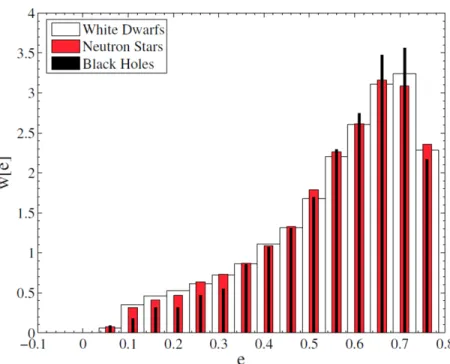
1.1 The probability distribution function of a compact object entering an eLISA-like passband vs. eccentricity. The mass of the super-massive black hole is taken to beM = 3×10⁶M. Image credit: Hopman and Alexander. . . 2 2.1 Efficiency of spectral source integration in comparison to ODE integration. The convergence
of normalization constantsC+with l= 2, m= 2, n= 0 is shown for various eccentricities in orbits withp= 10. The ODE integration uses the Runge-Kutta-Prince-Dormand 7(8) routine rk8pd of the GNU Scientific Library (GSL) . . . 21 3.1 The effectiveness of the diagonal Pade approximant (DPA) method for constructing
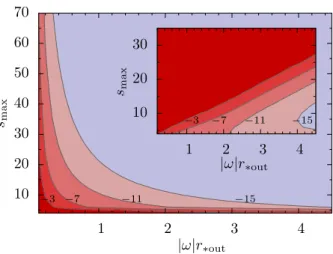
bound-ary conditions to the homogeneous Lorenz-gauge field equations compared to the standard asymptotic expansion. The relative error for each basis of homogeneous solutions is calculated with both methods and the worst case is reported. The contours are of constant relative error with log10 scaling, and are given as a function of the number of expansion terms smax and the location ofr∗. The larger plot shows the relative error of the DPA while the inset shows the relative error of the asymptotic expansion. It is apparent that the DPA allows initial conditions to be given at approximately a factor of 10 closer to the source region than the asymptotic expansion. The odd-parity case of (l, ω) = (2,10−4M−1) is shown. Similar results are observed for the even-parity sector. . . 35 3.2 Subdominance instability and growth of roundoff errors with starting location. The effects of
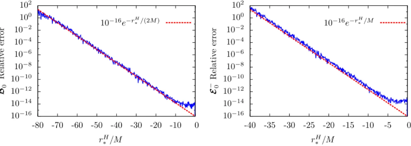
a subdominance instability are demonstrated by comparing results of numerical integrations begun at different initial radii rH
∗ near the horizon and ending at r∗ = 10M. The chosen modes havel= 2 andM ω= 1 (odd-parity on the left; even-parity on the right). The fiducial, accurate solution is obtained from a high-order Taylor expansion, with sufficient terms that residuals are at or below roundoff even at a radius ofrH
∗ = 0. Using the Taylor expansion at any −6M < rH
∗ <0 to begin an integration that then ends at r∗ = 10M gives results that are consistent with each other. However, as smaller initial radii are chosen (rH
∗ <−10M), exponentially greater errors are found in comparing at r∗ = 10M the integrated mode and the fiducial Taylor expansion. The instability is avoided by beginning all integrations at
rH
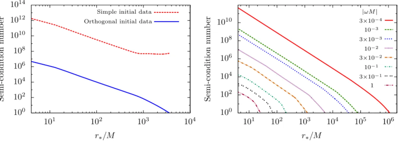
∗ =−6M with initial conditions from the high-order Taylor expansion. . . 44 3.3 Semi-condition number growth of outgoing homogeneous solutions and effect of thin-QR
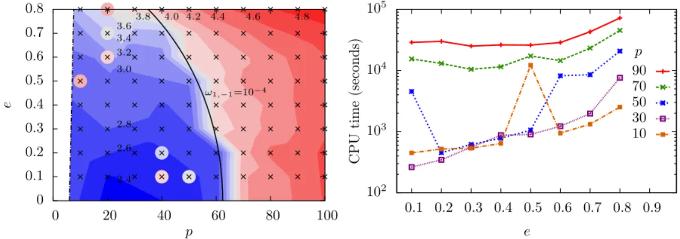
pre-conditioning. The left panel uses the even-parity mode (l, ω) = (5,5×10⁻³M−1) and plots as a function ofr∗ the semi-condition numberη of the matrixV, which is comprised of (the outer solution) half of the Wronskian matrix. Two initial conditions are compared: the simple basis in red (dotted) and the thin-QR pre-conditioned basis in blue (solid). Orthogonalization with the thin-QR pre-conditioner makes a more than five orders of magnitude improvement. The right panel uses an l = 16 even-parity mode and shows the growth of η in solutions that start with thin-QR orthogonalized initial conditions, as functions of frequency. Once the frequency reaches |ωM| ≤ 10−5, thin-QR pre-conditioning is no longer sufficient to control the condition number in the source region and still allow double precision computations, and other techniques are applied. . . 46 3.4 Plots of CPU time for self-force calculations as a function of orbital parameter space location.
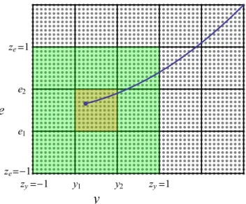
5.1 Data used for interpolation of the oscillatory self-force. Data was computed for 9,602 unique orbits at a cost of 2,308 CPU hours. Most of the gaps in the dataset correspond to orbital resonances where small (non-zero) Fourier-mode frequencies are encountered (these modes are difficult for the Lorenz-gauge code to compute). The adiabatic data is computed over approximately the same domain, but with four times the density and no gaps due to orbital resonances. Explicitly, adiabatic data was computed for 43,875 unique orbits at a cost of 2,054 CPU hours. . . 74 5.2 The local discretization used for interpolation over the (e, y) parameter space (see Eqn. (5.14)
for the defintion of y). The blue line represents the inspiral trajectory with a point at the current position. The yellow zone is the inspiral’s current sub-domain. The interpolation is performed with data (gray dots) from the yellow and green zones. . . 75 5.3 Estimates of interpolation error in the adiabatic part of self-force. The interpolation error of
Ft
adis estimated by computing orbits independent of those used for fitting interpolation coef-ficients and comparing with interpolated self-force values. The interpolation model recovers
Ft
adacross parameter space with an error no worse than∼10−8(better for lower eccentricities and away from the separatrix). Similar results are observed for the other components of the self-force. . . 76 5.4 Estimates of interpolation error in oscillatory part of self-force. The interpolation error ofFt
osc is estimated by computing orbits independent of those used for fitting interpolation coefficients and comparing with interpolated self-force values. The interpolation model recovers Ft
osc across parameter space with an error no worse than ∼ 10−3 (better for lower eccentricities and away from the separatrix). The larger error at high eccentricity is a limitation of the underlying data from the Lorenz-gauge code and motivates the hybrid scheme. Similar results are observed for the other components of the self-force. . . 77 5.5 Sensitivity of inspiral phase to error in the self-force. The sensitivity of the inspiral phase,
ϕp, to errors inFα
adandFoscα is tested by independently perturbing each part of the self-force with uniform errors of the indicated relative size, ∆. At a relative size of ∆, the expectation is that trial errors introduced in the adiabatic part of the self-force should have an effect that is a factor−1 larger than the effect of comparable errors injected in the oscillatory part of the self-force. The observed ratio is less dramatic but nevertheless indicates that computing the adiabatic part more accurately by orders of magnitude is crucial. The inspiral parameters were set to bee0 = 0.7, p0 = 10, χ00 = 0, and = 10−5. The timescale is set by assuming
M = 106M
. . . 78 5.6 Sensitivity in the evolution ofχ0 to self-force errors. To test the propagation of errors into
χ0, the force components in the χ0 evolution equation are perturbed while leaving the e andpevolution equations unaffected. Furthermore, errors are independently introduced into
Fcons and Fdiss in the χ0 equation. At the worst case error level, the dissipative self-force clearly has little influence on the evolution of χ0. Since only the dissipative part is affected by hybridization, the hybrid force is not essential in the evolution ofχ0. At this same error level, the conservative part is accurate enough to hold errors inχ0to 0.01 radians or less. The inspiral parameters were e0 = 0.7,p0 = 10,χ00= 0, and = 10−5. The timescale is set by assuming againM = 106M
5.7 Sample snapshots of an inspiral withM = 106M
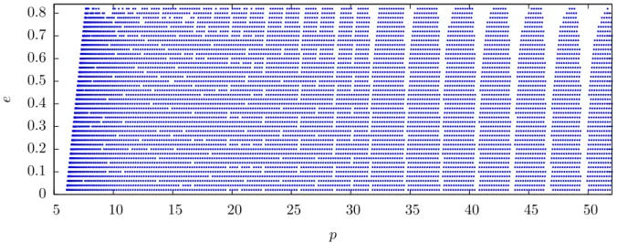
and = 10−5. The inspiral is plotted in Boyer-Lindquist coordinates with x = (rp/M) cos(ϕp), y = (rp/M) sin(ϕp). Each snapshot shows three periastron passages of the (counter-clockwise moving) inspiral and the central black hole is drawn to scale. The initial configuration is∼2,115.5 days from plunge and is shown in the top left panel. The initial parameters are p = 12, e = 0.81 (this corresponds to pM = 0.1183 AU). The other panels show 500 days until plunge (top right), 100 days to plunge (bottom left) and 1 day until plunge (bottom right). The inspiral depicted here corresponds to the second-from-the-left black curve in the Fig. 5.8. . . 80 5.8 Sample inspirals for µ/M = 10−5 and M = 106M
. Solid black curves show the evolution of (p, e) from entering the LISA-like passband (marked with the blue curve). This curve is truncated to a constant ineforp.16 because it is predicted that the initial eccentricity of EMRIs will not be above∼0.81. Generally, as each inspiral progresses, bothpandedecrease (with the exception of an increase ine near the separatrix). The dashed lines are contours that mark the number of radiansχ0 will evolve from a given point until plunge (this number is negative as the conservative self-force, and hence evolution of χ0, acts against the usual periastron advance). . . 81 5.9 Sample IMRI evolution. The evolution of the orbital frequencies for inspirals computed using
the full self-forceFα(red curve), the dissipative self-forceFα
diss(blue curve), and the adiabatic self-forceFα
LIST OF ABBREVIATIONS AND SYMBOLS
LIGO Laser Interferometer Gravitational-wave Observatory KAGRA Kamioka Gravitational Wave Detector
eLISA Evolved Laser Interferometer Space Antenna
M mass of the large black hole
M mass of the Sun
µ mass of the small compact object
ratio between the masses of the two bodies (µ/M) EMRI extreme-mass-ratio inspiral
IMRI intermediate-mass-ratio inspiral
e orbital eccentricity MP metric perturbation
Gµν Einstein tensor
gµν spacetime metric of the large black hole
pµν metric perturbation induced by the small compact object
Tµν stress-energy tensor of the small compact object
c speed of light
G Newton’s gravitational constant ¯
pµν trace-reversed metric perturbation ∇µ covariant derivative compatible with gµν 42 wave operator of the background spacetime
Rα βµ ν Riemann tensor compatible withgµν
uα small compact object’s four-velocity
Fα first-order gravitational self-force
pR
µν regular MP
pS
µν singular MP
Fα
Fα
diss dissipative part ofFα
Fadα adiabatic part of Fα
Fα
osc oscillatory part of Fα
Foscα(diss) dissipative part ofFoscα
φ waveform phase
κ mass-ratio expansion coefficients of Φ
xa Schwarzschild coordinates (t, r, θ, ϕ)
f 1−2M/r
τ proper time
zα
G worldline of a geodesic E specific orbital energy
L specific orbital angular momentum
e orbital eccentricity
p orbital semi-latus rectum
rmax radial position at apocenter
rmin radial position at pericenter
χ relativistic anomaly
χ0 value ofχat periastron
v χ−χ0
Tr radial period in coordinate time Tr radial period in proper time
∆ϕ azimuthal angle accumulated in one radial period Ωr fundamental radial frequency
Ωϕ mean azimuthal frequency det(gαβ) determinant of gαβ
δ Dirac delta function
m azimuthal number
Ylm spherical harmonic
Ylm
A even-parity vector-spherical-harmonic
Ylm
AB even-parity tensor-spherical-harmonic
Xlm
A odd-parity vector-spherical-harmonic
Xlm
AB odd-parity tensor-spherical-harmonic
hlm
ab even-parity tensor-spherical-harmonic amplitudes ofpµν
jlm
a even-parity tensor-spherical-harmonic amplitudes ofpµν
Klm even-parity tensor-spherical-harmonic amplitude ofp µν
Glm even-parity tensor-spherical-harmonic amplitude ofp µν
hlm
a odd-parity tensor-spherical-harmonic amplitudes ofpµν
hlm
2 odd-parity tensor-spherical-harmonic amplitude ofpµν ΩAB metric of unit two-sphere
Qab
lm even-parity tensor-spherical-harmonic amplitudes ofTµν
Qa
lm even-parity tensor-spherical-harmonic amplitudes ofTµν
Q]lm even-parity tensor-spherical-harmonic amplitude ofTµν
Q[
lm even-parity tensor-spherical-harmonic amplitude ofTµν
Plma odd-parity tensor-spherical-harmonic amplitudes ofTµν
Plm odd-parity tensor-spherical-harmonic amplitude ofTµν
λ (l+ 2)(l−1)/2 Ξµ gauge vector
ξlm
a even-parity spherical harmonic amplitudes of Ξµ
ξlm even-parity vector-spherical-harmonic amplitude of Ξµ
ξlm
2 odd-parity vector-spherical-harmonic amplitude of Ξµ
RW Regge-Wheeler
Ψ even- or odd-parity master function
2 1 + 1 dimensional d’Alembertian
V even- or odd-parity effective potential
S even- or odd-parity master-function source
r∗ tortoise coordinate
G even- or odd- parity delta function source amplitude
F even- or odd- parity derivative-of-delta function source amplitude
n radial Fourier harmonic number
ωmn mΩϕ+nΩr(angular frequency in radians/second) ODE ordinary differential equation
˜
Ψ± Homogeneous master function solutions in the frequency domain
c±(r) RW normalization functions
C± RW normalization constants Θ Heaviside step function
EHS extended homogeneous solutions
Ψ± RW EHS
SSI spectral source integration
I arbitrary integral with smooth and periodic integrand
g integrand ofI
˜
Gn Fourier series spectrum ofg
ν oscillation frequency (in Hertz)
B bandwidth
N number of time samples
¯
G GeimΩϕt
¯
F F eimΩϕt
¯
E argument of Fourier transform for normalization constants
tj jTr/N
˜
En0 Fourier series amplitude of ¯E En0 DFT amplitude of ¯E
hE˙i time-averaged energy flux
hL˙i time-averaged angular momentum flux
E vector of even-parity MP amplitudes
B vector of odd-parity MP amplitudes
A even-parity derivative coupling matrix
B even-parity coupling matrix
C odd-parity derivative coupling matrix
D odd-parity coupling matrix ˜
U even-parity source vector ˜
V odd-parity source vector
k dimension of ˜E or ˜B
I identity matrix
˜
E±i even-parity homogeneous solution ˜
B±i odd-parity homogeneous solution
σ ωM
s exponent of power series expansion term
a()s coefficient of near-horizon expansion term
A()s right-hand-side of near-horizon recurrence relation
b()s coefficient of near-infinity expansion term
Bs() right-hand-side of near-infinity recurrence relation
smax number of terms in a near-infinity expansion DPA diagonal Pade approximant
α() near-infinity DPA expansion
βs() DPA numerator coefficient
γs() DPA denominator coefficient
r∗out large positiver∗ for testing expansions
ce/o,i ± even- or odd-parity normalization function
M Wronskian matrix
0 zero vector
We/o determinant of Wronskian matrix
Wie/o determinant of modified Wronskian matrix
LU lower-upper
Cie/o,± even- or odd-parity normalization constant ˜
v time-domain Dirac delta function amplitude of ˜V
v v˜eimϕp
¯
E vector argument of SSI
αi roundoff error coefficient
βi roundoff error coefficient
rH
∗ large negativer∗starting position of ODE integration
r∞
∗ large positiver∗ starting position of ODE integration
κ condition number
λmax/min extremal eigenvalues of M
σi singular values
η semi-condition number
J vector describing the jump in ∂rBat the particle location ˜
h±t homogeneous odd-parity static mode
aodd
bodd
s expansion coefficient for ˜h+t
Hs thesth harmonic number
dodd
s alternative expansion coefficient for ˜h+t
Γ Gamma function
Sξ± source term for the even-parity static inhomogeneous gauge solution ˜
ξ±H0/1 homogeneous gauge solution for even-parity static modes ˜
ξ±I inhomogeneous gauge solution for even-parity static modes
∆˜ξ even-parity static mode gauge generator
∆˜ξH 0/1
±
homogeneous even-parity static mode gauge generator
∆˜ξI
±
inhomogeneous even-parity static mode gauge generator
aHs 0/1 expansion coefficient for ˜ξH−0/1
bHs 0/1 expansion coefficient for ˜ξH+0/1
dHs 0/1 alternative expansion coefficient for ˜ξ+H0/1
y±
s expansion coefficient forS±ξ
aI
s expansion coefficient for ˜ξI−
bI
s expansion coefficient for ˜ξI+
vs alternative expansion coefficient forSξ±
dIs alternative expansion coefficient for ˜ξ + I
kαβγδ self-force projection operator
Fα
ret divergent self-force constructed frompµν without regularization
Fα
S divergent self-force constructed frompSµν
Fαl0
ret scalar-spherical-harmonic (l0) mode ofFretα
FSαl0 scalar-spherical-harmonic (l0) mode ofFSα
Fα
[i] regularization parameter
fαlm
i tensor-spherical-harmonic modes of Fretα F(j)αl,m certain linear combinations of fiαlm
U2
Fα
R,ret alternate notation forFα
FR,advα regularized self-force calculated frompadvµν
Fα
adv divergent self-force constructed frompadvµν without regularization
Fαl0
adv scalar-spherical-harmonic modes ofFadvα
(α) (-1,1,1,-1) ˜
an cosine Fourier series (τ) coefficient ofFα ˜bn sine Fourier series (τ) coefficient ofFα
Fhyb
α hybrid (covariant) self-force ˜
gn cosine Fourier series (v) coefficient ofFα ˜
hn sine Fourier series (v) coefficient ofFα
Ij (p, e, χ
0, tp, ϕp)
a(µ) self-force coefficient foreevolution equation
b(µ) self-force coefficient forpevolution equation
c(µ) self-force coefficient forχ0evolution equation
q denominator of e,p, andχ0evolution equations
x p−2e−6
y orbital parameter that depends only on x w smooth transistion function
d width of smooth transition function
aα
n cosine Fourier series (v) coefficient ofFα
bα
n sine Fourier series (v) coefficient ofFα
e1 leading edge of interpolation sub-domain (e)
e2 trailing edge of interpolation sub-domain (e)
ze (2e−e2−e1)/(3(e2−e1))
y1 leading edge of interpolation sub-domain (y)
y2 trailing edge of interpolation sub-domain (y)
Ti Chebyshev polynomial of the first kind
σαnij Chebyshev coefficient
∆ trial error for testing the sensitivity of the phase to different self-force components
a specific angular momentum of a Kerr black hole ρ r2+a2cos2θ
∆ r2−2M r+a2
R square of rate of change of Kerr rmotion
Θ square of rate of change of Kerr θmotion
Φ rate of change of Kerr ϕmotion
T rate of change of Kerr tmotion
Lz z-component of specific orbital angular momentum
Q Carter constant
r1 rmax
r2 rmin
r3 third largest root ofR(rp) = 0
r3 fourth largest root ofR(rp) = 0
p3 r3(1−e)/M
p4 r4(1 +e)/M
ι inclination angle
λ Mino time
z± square of the cosine of the roots ofΘ(θp) = 0
ψ alternate parameter for describing θp β a2(1− E2)
λ(r) Mino time as a function ofχ
λ(θ) Mino time as a function ofψ
P(r) rate of change of λ(r)
P(θ) rate of change of λ(θ) Pj(r/θ) Fourier amplitude of P(r/θ) Λr radial period measured withλ Λθ polar period measured withλ
Υr radial fundamental frequency measured withλ Υθ polar fundamental frequency measured with λ Pkn(t) Fourier amplitude of T
Pkn(ϕ) Fourier amplitude of Φ
T(r) part of Tthat depends only onr p
T(θ) part of Tthat depends only onθ p
Φ(r) part of Φthat depends only onr p
Φ(θ) part of Φthat depends only onθ p
Tn(r) Fourier amplitude of T(r) Tk(θ) Fourier amplitude of T(θ)
℘(r)n Fourier amplitude of Φ(r)
℘(θ)k Fourier amplitude of Φ(θ)
ψj discretized list ofψ values
Γ average rate of change oftprelative to λ Υϕ average rate of change ofϕp relative toλ Ωθ fundamental polar frequency according to t
Φ scalar field
T scalar charge density q scalar charge
Xlmkn radial separation function for Φ
Slmkn polar separation function for Φ, or the spheroidal Legendre function ˜
Tlmkn Fourier and spheroidal harmonic amplitude ofT
Ulmkn scalar Teukolsky potential ˜
Almkn modified spheroidal harmonic amplitude ofT
X± homogeneous radial Teukolsky solutions
γ near-horizon wavenumber of X− ˜
B re-factored version of ˜A
˜
C modified version of ˜B for a Mino time Fourier transform ˜
D± C˜ modified to includeX∓ ˜
K± radial part of ˜D±
˜
J polar part of ˜D±
I1± integral used for calculatingC±
I2 integral used for calculatingC±
I3± integral used for calculatingC±
CHAPTER 1: Introduction
Section 1.1: Motivation
The era of gravitational wave astronomy has dawned, and relativistic compact binary systems are one important class of emitters [1]. Current and future gravitational wave experiments include the Laser Inter-ferometer Gravitational-wave Observatory (LIGO) [2], which made the pioneering laboratory gravitational wave detection [1], the Virgo interferometer [3], the Kamioka Gravitational Wave Detector (KAGRA) [4], and the Evolved Laser Interferometer Space Antenna (eLISA) [5], which is a planned space mission by the European Space Agency. Accurate theoretical models are vital to the detection of gravitational waves [1, 6] and, upon detection, determining the physical systems that emitted them. Observation of gravitational wave sources will inform population studies of compact objects and will allow further precision tests of general relativity in the strong-field regime.
Producing accurate theoretical models requires solving the two body problem of general relativity, which, unlike its Newtonian counterpart, does not have a known solution in closed form. A number of different techniques exist to approximate solutions to this problem, each applicable to a different class of system depending upon the orbital separation or the mass-ratio of the two bodies. When the two bodies are widely separated, the post-Newtonian expansion can be employed [7]. This expansion performs well in the slow adiabatic phase of the inspiral but becomes less accurate as the orbital separation decreases. Once the strong-field regime is entered, for comparable-mass systems, no analytic approximations can be made and the full non-linear Einstein equations must be solved on a supercomputer through numerical relativity [8, 9]. The discovery of gravitational waves by Advanced LIGO was facilitated by numerical relativity simulations of comparable mass black holes [1]. More extreme-mass-ratio systems are beyond the current reach of numerical relativity due to the high resolution requirements around the smaller body and the wide separation of time scales in the problem. In this regime one turns to black hole perturbation theory and self-force calculations [10–12]. In addition there is effective-one-body theory [13–15], which incorporates elements from all three of the aforementioned schemes. This work advances state-of-the-art black hole perturbation theory and self-force calculations to improve modeling of small-mass-ratio binary systems relevant to gravitational wave observations.
Section 1.2: Astrophysical considerations
Extreme-mass-ratio inspirals (EMRIs) consist of a super-massive (M ∼105–107M
Figure 1.1: The probability distribution function of a compact object entering an eLISA-like passband vs. eccentricity. The mass of the super-massive black hole is taken to beM = 3×10⁶M
. Image credit: Hopman and Alexander [18].
EMRIs have a mass-ratio of= 10−4–10−7. Super-massive black holes are found in the center of most galaxies [16] and are expected to be rotating rapidly [17] (with|angular momentum| ∼M2). Stellar remnants form the smaller compact objects. When a small compact object encounters other bodies in the galactic nucleus it can be scattered into a nearly radial trajectory (bound but extremely eccentric). If the compact object avoids additional encounters for a long enough duration then the orbit will tighten due to radiative (gravitational) losses until it enters the eLISA passband. The eccentricity distribution of compact objects entering the eLISA passband through this mechanism is thought to be peaked around e' 0.6−0.8 (see Fig. 1.1 and Ref. [18]). Past attempts to model EMRIs (beyond the adiabatic approximation) have been limited to small eccentricities (e≤0.2) for technical reasons [19]. Therefore, a primary goal of this work is to overcome the problems associated with high eccentricity and model inspirals up toe'0.8. EMRIs are expected to provide clean tests of general relativity in the strong-field regime [20–23] (unspoiled by environmental effects [24]).
Intermediate-mass-ratio inspirals (IMRIs) are those with a mass ratio of = 10−1–10−4. For IMRIs to occur, intermediate-mass black holes must exist with masses M ∼102–104M
a super-massive black hole. The latter configuration would produce a very strong gravitational wave signal in the eLISA passband [26]. The former configuration could produce a signal in the passband of Advanced LIGO.
Section 1.3: Modeling EMRIs and IMRIs
Modeling EMRIs and IMRIs is achieved by perturbatively expanding the Einstein field equations in powers of the (small) mass-ratio . Typically, the smaller body is modeled as a point particle and the particle’s interaction with its metric perturbation (MP) gives rise (after regularization) to a self-force that drives the inspiral [27–32]. Calculating this self-force has been a major research effort for the past 15 years that has met with great success, both in computing the gravitational self-force [33–38] and conservative gauge-invariant quantities [39–42], which have been compared with results from other approaches to the two-body problem [43–54].
This work considers perturbative solutions to the Einstein equations through first-order in
Gαβ h
gµν+pµν+O(2) i
= 8πTαβ, (1.1)
where Gαβ is the Einstein tensor as a function of the spacetime metric,gµν is the spacetime metric of the large black hole, pµν is the MP induced by the small compact object, and Tαβ is the stress-energy tensor of the small compact object. Units are adopted in which c = G = 1 (the speed of light and Newton’s gravitational constant are unity), and the sign conventions of Misner, Thorne, and Wheeler [55] are followed throughout. It is convenient to introduce the trace-reversed MP ¯pµν
¯
pµν =pµν−12gµν(pαβgαβ) (1.2)
and adopt the Lorenz gauge condition
∇µp¯µν = 0, (1.3)
where indices are raised and lowered withgµν, and∇µis the covariant derivative compatible withgµν. Eqns. (1.1) and (1.3) imply the following field equations for ¯pµν [56]
42¯p
µν+ 2Rα βµ νp¯αβ=−16πTµν, (1.4)
where42=gµν
In principle, the small object’s motion is geodesic in the spacetime with metricgµν+pµν. An equivalent interpretation is that of forced motion in the background spacetime (with metricgµν). In either interpreta-tion, the small object’s trajectory evolves according to
µuβ
∇βuα=Fα+O(3), (1.5)
whereuβ is the small object’s four-velocity andFα is the first-order gravitational self-force [11]
Fα=−µ 2 g
αβ+uαuβ
(2∇µpνβ − ∇βpµν)uµuν. (1.6)
However, pµν diverges at the position of the small object (Coulomb-like divergence), so Eqn. (1.6) does not result in a physically reasonable force. This divergence is a consequence of treating the small object as a point-particle. A realistic description of the small object as an extended (but compact) body or black hole provides the solution. The metric in the neighborhood of the small object is taken to be that of a compact physical body in the tidal field of the large black hole. By matching this metric to the background spacetime (perturbed by the moving body) and requiring that the configuration satisfy Einstein’s equations, the correct self-force is obtained [11, 27, 28]. One elegant interpretation is to decompose the (retarded) MP into a regular part, pR
µν, that is responsible for the self-force and a singular part, pSµν, that diverges but formally does not contribute to the force [30]
pµν =pRµν+pSµν. (1.7)
The correct self-force is given by usingpRµν with (1.6)
Fα=
−µ2 gαβ+uαuβ
2∇µpRνβ − ∇βpRµν
uµuν. (1.8)
In this work, the self-force is calculated by assuming the small object has followed a background geodesic for its entire history. This introduces an approximation because its actual inspiral trajectory differs from a geodesic in the distant past. There is ongoing work to quantify the error induced by making this ap-proximation [57–59]. In the geodesic self-force scheme the force can be split into a conservative partFα
cons, attributed to the time-symmetric part of the gravitational field, and a dissipative part Fα
diss, due to the time-antisymmetric part of the gravitational field
The dissipative part is responsible for radiation reaction effects such as decay of the orbital energy and angular momentum. The conservative part perturbs the orbital parameters, but does not cause a secular decay of the orbit. The dissipative self-force can be further split into two parts: an adiabatic partFadα, whose components vary slowly over an inspiral on the radiation reaction timescale and represents some average over the orbital timescale, and an oscillating part Foscα(diss), whose components oscillate on the orbital timescale. Thus, the full self-force can be written as
Fα=Fadα +Foscα , (1.10)
Fα
osc≡Foscα(diss)+Fconsα . (1.11)
A rigorous discussion of how the different parts of the self-force influence the inspiral phase is given by Hinderer and Flanagan [60], and the following section reviews some key results.
Section 1.4: Accuracy requirements for inspirals into a Schwarzschild black hole
With an E/IMRI there is a large accumulation of orbital phase from the point when the binary enters the eLISA passband until merger. The leading-order part of the orbital phase enters atO(−1) and is driven by the abovementioned adiabatic, first-order-in-the-mass-ratio, dissipative self-forceFα
ad. Conveniently, this component of the self-force can be related to the orbit-averaged asymptotic fluxes (and rate of change of the Carter constant [61]), which sidesteps the need for a more complicated, local calculation of the self-force from the metric perturbation at the particle. A number of authors have used this adiabatic approach to calculate the leading-order phase evolution of generic inspirals into Kerr black holes [62, 63], though at the cost of missing some effects available within the first-order perturbation.
To summarize, the influence of each component of the self-force on the phase of the waveformφis
φ= κ0−1 | {z } adiabatic: Fα
ad
+ κ1/2−1/2 | {z } resonances (Kerr only)
+ κ10 | {z } post-1-adiabatic: Fα
osc+ 2ndorder avg.
+ · · · , (1.12)
where the κ coefficients are dimensionless, of order unity, and do not depend on the mass ratio . The adiabatic part of the self-force comes in at lower order than the remaining parts of the self-force, and accordingly must be computed with greater accuracy in order to affect the phase error at the same level. In order to aid in the detection of gravitational waves from an EMRI while correctly determining the configuration of their source, φwill need to be calculated to within∼0.1 radians. To achieve this goal for an = 10−5 inspiral into a Schwarzschild black hole, Fα
ad will need be accurate to at least ∼7 digits and
Fα
osc will need to be accurate to at least ∼2 digits. One challenge faced when calculatingFα is that Fadα and Fα
osc are obtained simultaneously, so it is non-trivial to take advantage of this separation of accuracy requirements.
Section 1.5: Organization of this work
Chapter 2 introduces the formalism used to calculate Schwarzschild metric perturbations. A simple gauge choice is made (Regge-Wheeler gauge) to demonstrate a novel technique by Hopper, Forseth, Osburn, and Evans [72] for calculating Schwarzschild black hole perturbations at spectral accuracy (exponential convergence of numerical calculations) that was developed as a part of this work. This technique is used here to calculate (from fluxes) the leading contribution to the self-force,Fα
ad, with the required high accuracy (7+ digits).
Chapters 3-4 report new results from Osburn, Forseth, Evans, and Hopper [65] that apply Lorenz gauge metric perturbations to calculate Fα
osc. A series of novel techniques, including a pre-conditioning technique for initial data (for numerical integrations), are introduced to overcome an inherent ill-conditioning problem. These techniques allowFα
oscto be calculated at orbital eccentricities and separations never before achieved. Chapter 5 reports new results from Osburn, Warburton, and Evans [73] that apply techniques described in Chapters 2-4 to drive the evolution of small mass-ratio inspirals. It is demonstrated that a hybrid method, where Fα
ad and Foscα are calculated separately (and each to their own required tolerance), and other novel optimizations make it possible to monitor the waveform phase at observationally-motivated accuracies never achieved before and to do so for observationally-motivated orbital configurations.
CHAPTER 2: Perturbations of a Schwarzschild black hole
The work discussed in this chapter is largely drawn from Refs. [72, 74].
Section 2.1: Bound geodesic motion in Schwarzschild spacetime
The MP will be sourced by a point mass in geodesic motion around a Schwarzschild black hole. Schwarzschild coordinatesxα= (t, r, θ, ϕ) are adopted, in which the line element takes the standard form
ds2=
−f dt2+f−1dr2+r2 dθ2+ sin2θ dϕ2
, (2.1)
wheref(r) = 1−2M/r. The geodesic worldline is given by a set of functionszα
G(τ) = [tp(τ), rp(τ), θp(τ), ϕp(τ)], parameterized by (for example) proper timeτ. Without loss of generality the motion is confined to the equa-torial plane,θp=π/2. The geodesic four-velocityuαis given by
uα=
E
fp
, ur,0, L r2 p
, (2.2)
wherefp≡f(rp) andE andLare the specific energy and angular momentum, respectively. The constraint on the four-velocityuαu
α=−1 yields an expression forur:
(ur)2=E2−fp
1 +L 2
r2 p
. (2.3)
The geodesic is parameterized with the eccentricity, e, and dimensionless semi-latus rectum, p, which are related to the radial turning pointsrmin andrmax via
p= 2rmaxrmin
M(rmax+rmin)
, (2.4)
e=rmax−rmin
rmax+rmin.
Eqn. (2.4) and the roots of Eqn. (2.3) give the relationship between (p,e) and (E,L):
E = s
(p−2)2−4e2
p(p−3−e2), (2.5)
L=p pM
Orbits are bound whene <1 and are stable whenp >6 + 2e.
In self-force calculations it is convenient to reparameterize the orbital motion (i.e., all the curve functions) with the relativistic anomalyχ[75], defined so that
rp(χ) = pM
1 +ecos [χ−χ0]. (2.6)
The parameterχ0specifies the value ofχ at pericentric passage.
Eqn. (2.6) can be used with Eqns. (2.2) and (2.5) to derive the following initial value equations for the development of the orbit
dτp
dχ =
M p3/2 (1 +ecosv)2
s
p−3−e2
p−6−2ecosv, (2.7)
dtp
dχ =
r2 p
M(p−2−2ecosv) s
(p−2)2−4e2
p−6−2ecosv, (2.8)
dϕp
dχ =
r p
p−6−2ecosv, (2.9)
where v ≡χ−χ0. Without loss of generality the following initial conditions can be chosen: ϕp|χ=0 = 0,
tp|χ=0= 0,τp|χ=0= 0, in which case χ0 serves to orient the orbit.
The periods of one radial libration measured intandτ are denoted byTrandTr, respectively. They are given by
Tr= Z 2π
0
dtp
dχdχ, Tr=
Z 2π
0
dτp
dχdχ. (2.10)
The amount of azimuthal angle accumulated in one radial period,Tr, is given by
∆ϕ= Z 2π
0
dϕp
dχdχ. (2.11)
Each orbit has associated with it two fundamental frequencies. One is a libration-type frequency associated with the radial motion and the other is a rotation-type frequency associated with the average rate at which the orbital azimuthal angle accumulates. These two frequencies are defined by
Ωr≡ 2π
Tr
, Ωϕ≡∆ϕ
Tr
Section 2.2: Field equations and tensor-spherical-harmonic decomposition
The finite mass of the small body induces a first-order perturbationpµν in the background metricgµν
Gαβ h
gµν+pµν+O(2) i
= 8πTαβ. (2.13)
This reduces to a system of 10 coupled linear hyperbolic partial differential equations for the components of
pµν [56, 76]
42(p
µν−pαβgαβ) +∇µ∇ν(pαβgαβ) + 2Rα βµ νpαβ− ∇ν∇αpµα− ∇µ∇αpνα+gµν(∇α∇βpαβ) =−16πTµν. (2.14)
The stress energy tensor is
Tµν(xα) =µ
Z uµuν p
−det(gαβ)δ(t−tp)δ(r−rp)δ(θ−θp)δ(ϕ−ϕp)dτ, (2.15)
where det(gαβ) is the determinant ofgαβ andδis the Dirac delta function.
In Schwarzschild spacetime, this system is separable into tensor-spherical-harmonic modes. The notation of Martel and Poisson [77] is followed, a modification of the original notation of Regge and Wheeler [78] (an alternative notation is found in [33, 36, 56]). This convention leaves all tensor-spherical-harmonics orthogonal and clarifies the distinction between even-parity and odd-parity amplitudes. Odd-parity perturbations are expanded in terms ofXlm
A andXABlm, while even-parity perturbations useYlm,YAlm, and YABlm
pab= X
lm
hlmab(t, r)Ylm(θ, ϕ),
paB= X
lm
jalm(t, r)YBlm(θ, ϕ) +hlma (t, r)XBlm(θ, ϕ)
, (2.16)
pAB= X
lm
r2 Klm(t, r) ΩABYlm(θ, ϕ) +Glm(t, r)YABlm(θ, ϕ)
+hlm2 (t, r)XABlm(θ, ϕ)
.
Lowercase Latin subscripts and superscripts (a, b) run overt and r while uppercase Latin subscripts and superscripts (A, B) run over θ and ϕ. The seven even-parity tensor-spherical-harmonic amplitudes are
hlm
tt , hlmtr, hlmrr, Klm, jtlm, jrlm, andGlm. The three odd-parity tensor-spherical-harmonic amplitudes arehlmt , hlmr , andhlm
2 . The metric on the unit two-sphere is ΩAB. The stress-energy tensor is also decomposed following [77] and has even-parity projections
Qab
lm(t, r) = 8π Z
Qalm(t, r) = 8πr2
λ+ 1 Z
TaBY¯BlmdΩ, (2.17)
Q[lm(t, r) = 8πr2 Z
TABΩABY¯lmdΩ, Q]lm(t, r) = 8πr
4
λ(λ+ 1) Z
TABY¯ABlmdΩ,
and odd-parity projections
Plma (t, r) = 8πr2
λ+ 1 Z
TaBX¯BlmdΩ,
Plm(t, r) = 4πr 4
λ(λ+ 1) Z
TABX¯ABlm dΩ. (2.18)
The overbar here indicates the complex conjugate and λ ≡ (l+ 2)(l−1)/2. The sharp (]) and flat ([) superscripts merely distinguish two distinct projections. These source terms are given explicitly in Sec. V of [74]. The projections of (2.14) are given by [77].
Section 2.3: Gauge transformations
In general relativity, gauge transformations are equivalent to a change of coordinate system. In this work, coordinate transformations will be treated perturbatively
xµ→xµ+ Ξµ+O(2). (2.19)
The gauge vector Ξµ can be decomposed into vector-spherical-harmonics with four amplitudes
Ξa =X lm
ξalm(t, r)Ylm(θ, ϕ), (2.20)
ΞA=X lm
ξlm(t, r)YAlm(θ, ϕ) +ξ2lm(t, r)XAlm(θ, ϕ)
.
Unless otherwise noted, further l and m indices will be suppressed. Eqns. (2.14) and (2.19) imply the following transformation equations for the (l, m) amplitudes ofpµν
htt→htt−2∂tξt+ 2M f
r2 ξr,
htr→htr−∂rξt+ 2M
r2 ξt−∂tξr,
hrr →hrr− ∂rξr−2M
r2fξr,
K→K−2f r ξr+
l(l+ 1)
r2 ξ,
jr→jr−ξr−∂rξ+2
rξ,
G→G−r22ξ,
ht→ht−∂tξ2,
hr→hr−∂rξ2+ 2
rξ2,
h2→ −2ξ2.
To calculate the gravitational self-force,ξa,ξ, andξ2are fixed such that the Lorenz gauge condition, Eqn. (1.3), is satisfied. Lorenz gauge is convenient because it is straightforward to regularize the self-force in that gauge. Another convenient gauge is Regge-Wheeler (RW) gauge, which satisfies the following conditions
jtRW=jrRW=GRW=hRW2 = 0. (2.22)
It is clear that ξa, ξ, and ξ2 can be chosen such that the RW gauge condition is satisfied. RW gauge is convenient because the field equations for each parity and multipole mode reduce to a single hyperbolic equation for a master function. The master function is used to construct the MP and calculate the energy and angular momentum fluxes.
Section 2.4: RW gauge metric perturbations
Applying the tensor-spherical-harmonic projections of Eqn. (2.16) to Eqn. (2.14) and enforcing the RW gauge condition yields coupled sets of field equations intandrfor the MP amplitudes [77]
Qtt=−∂r2KRW−
3r−5M r2f ∂rK
RW+f
r∂rh
RW rr +
(λ+ 2)r+ 2M
r3 h
RW rr +
λ r2fK
RW,
Qtr =∂t∂rKRW+
r−3M r2f ∂tK
RW
−fr∂thRWrr −
λ+ 1
r2 h RW tr ,
Qrr =−∂t2KRW+
(r−M)f r2 ∂rK
RW+2f
r ∂th
RW tr −
f r∂rh
RW tt +
(λ+ 1)r+ 2M
r3 h
RW tt −
f2
r2h RW rr −
λf r2K
RW,
Q[=−∂t2hRWrr + 2∂t∂rhRWtr −∂r2hRWtt − 1
f∂
2
tKRW+f ∂r2KRW +2(r−M)
r2f ∂th RW tr −
r−3M r2f ∂rh
RW tt +
2(r−M)
r2 ∂rK RW
−(r−rM2 )f∂rh RW
rr (2.23)
+(λ+ 1)r 2
−2(λ+ 2)M r+ 2M2
r4f2 h
RW tt −
(λ+ 1)r2
−2λM r−2M2
r4 h
RW rr ,
Pt=
−∂t∂rhRWr +∂r2hRWt − 2
r∂th
RW r −
2(λ+ 1)r−4M
r3f h
RW t ,
Pr=∂t2hRWr −∂t∂rhRWt + 2
r∂th
RW t +
2λf r2 h
It can be shown using Eqn. (2.23) and the Bianchi identities [77] that it is possible to construct the MP from a single master function (for each parity). The even-parity MP can be constructed from the Zerilli-Moncrief master function Ψeven [79]
Ψeven= r
λ+ 1
KRW+ f Λ
f hRW
rr −r∂rKRW
, (2.24)
KRW=f ∂rΨeven+ 1
rΛ
λ(λ+ 1) +3M
r
λ+2M
r
Ψeven− r 2f2
(λ+ 1)ΛQ
tt, (2.25)
hRWrr = Λ
f2
λ+ 1
r Ψeven−K
RW
+r
f∂rK
RW, (2.26)
hRWtr =r∂t∂rΨeven+ 1
fΛ
λ
1−3M
r
−3M
2
r2
∂tΨeven− r 2
λ+ 1
Qtr+rf Λ∂tQ
tt, (2.27)
hRWtt =f2hRWrr +f Q], (2.28)
where Λ = λ+ 3M/r, and the odd-parity MP can be constructed from the Cunningham-Price-Moncrief master function Ψodd [80]
Ψodd= r
λ
∂rhRWt −∂thRWr − 2
rh
RW t
, (2.29)
hRWt =
f
2∂r(rΨodd)−
r2f 2λP
t, (2.30)
hRWr =
r
2f∂tΨodd+ r2
2λfP
r. (2.31)
Unless otherwise noted, “even” and “odd” subscripts will be further suppressed. The master functions satisfy a hyperbolic partial differential equation, and the principal part of the wave operator can be compactly expressed using the 1+1 dimensional d’Alembertian2
2
−V(r)
Ψ(t, r) =S(t, r), (2.32)
2=−∂2
t +f ∂r(f ∂r), (2.33)
=−∂t2+∂r2∗,
Veven=
f r2Λ2
2λ2
λ+ 1 +3M
r
+18M
2
r2
λ+M
r
, (2.34)
Vodd = f
r2
l(l+ 1)−6Mr
, (2.35)
where the “prime” (δ0) indicates anr derivative andr∗ is the tortoise coordinate
r∗=r+ 2Mln r
2M −1
. (2.37)
The fully-evaluated even- or odd-parity source amplitudesF andGare given by [74]. In the source-free case, the odd-parity form of Eqn. (2.32) is the homogeneous RW equation [78], and the even-parity form of Eqn. (2.32) is the homogeneous Zerilli equation [76].
Section 2.5: Fourier decomposition
As explained in Sec. 2.1, two fundamental frequencies, Ωrand Ωϕ, exist in the eccentric-orbit Schwarzschild E/IMRI problem. In the frame that rotates at the mean azimuthal rate (ϕ0 = ϕ−Ωϕt) the MP appears non-sinusoidal but periodic in t. It can be represented in a Fourier series in harmonicsnΩr. In the inertial frame, the phase of each multipole with m 6= 0 advances linearly, giving the Fourier-harmonic modes a spectrum
ωmn=mΩϕ+nΩr. (2.38)
Each MP and source amplitude is replaced by a Fourier series (with a tilde denoting a frequency-domain amplitude). For the master function Ψ, the decomposition takes the following form
˜
Ψlmn(r) = 1
Tr Z Tr
0
Ψlm(t, r)eiωmntdt, (2.39)
Ψlm(t, r) = ∞ X
n=−∞ ˜
Ψlmn(r)e−iωmnt. (2.40)
The hyperbolic partial differential equation for Ψlm reduces to an ordinary differential equation (ODE) for every frequencyωmn
d2Ψlmn˜
dr2 ∗
+
ωmn2 −V(r) ˜
Ψlmn= ˜Slmn(r). (2.41)
Henceforth, not only will indicesl andmbe suppressed but so willn(unless otherwise noted). Eqn. (2.41) has two independent homogeneous solutions, ˜Ψ+(r) and ˜Ψ−(r), with the following asymptotic behavior
˜
Ψ±(r∗→ ±∞)∼e±iωr∗. (2.42)
Initial conditions for ˜Ψ±are given nearr
[81, 82].
Section 2.6: Variation of parameters and extended homogeneous solutions
The method of variation of parameters can be used to construct the particular solution. A Green’s function is formed from the two linearly independent solutions ( ˜Ψ+and ˜Ψ−) and integrated over the source function ˜S(r) to obtain the particular solution of (2.41)
˜
Ψ(r) =c+(r) ˜Ψ+(r) +c−(r) ˜Ψ−(r), (2.43)
where the normalization functions in the source region are given by the integrals
c+(r) = 1
W
Z r rmin
˜
Ψ−(r0) ˜S(r0)
f(r0) dr0,
c−(r) = 1
W
Z rmax
r ˜
Ψ+(r0) ˜S(r0)
f(r0) dr0.
(2.44)
HereW is the determinant of the Wronskian matrix
W = Ψ˜−dΨ˜ +
dr∗ − ˜ Ψ+dΨ˜−
dr∗ !
. (2.45)
While the expression in Eqn. (2.43) is indeed a solution to Eqn. (2.41), it is not ideal. The singular nature of the time-domain source (2.36) results in Gibbs behavior in the Fourier synthesis (2.40) of Ψ at and near the particle location, leading to slow algebraic convergence. Exponential convergence can be restored by using the method of extended homogeneous solutions (EHS), originally developed by Barack, Ori, and Sago [83].
The first step in EHS is to extend the limits of integration in (2.44) to include the full source region and obtain the normalization coefficients
C±= 1
W
Z rmax
rmin
˜
Ψ∓(r) ˜S(r)
f(r) dr. (2.46)
These complex constants are used to normalize the mode functions, which collectively encode all the infor-mation about the source motion and are used to define the EHS
Ψ±lm(t, r)≡X n
Clmn± Ψ˜±lmn(r)e−iωmnt. (2.47)
EHS
Ψ(t, r) = Ψ+(t, r) Θ [r−rp(t)] + Ψ−(t, r) Θ [rp(t)−r], (2.48)
where Θ is the Heaviside step function. This weak solution can be computed everywhere, including the particle location, and it allows the metric and local gravitational self-force to be accurately determined [74]. There remains the practical issue of computing the C±. For the RW problem, the source S(r) in Eqn. (2.46) is poorly behaved at the turning points because of the presence of theδ0 term in (2.36) [74]. It was shown in that paper that the problem could be circumvented by reversing the order of integration (see related examples in [83, 84]). To see this, substitute the Fourier transform integral for ˜S(r) into (2.46)
C±= 1
W
Z rmax
rmin
˜ Ψ∓(r)
f(r) 1
Tr Z Tr
0
S(t, r)eiωtdt
!
dr. (2.49)
Then substitute for the time-domain sourceS(t, r) its singular form (2.36), exchange the order of integration, and integrate in rover the delta function terms. What remains of the calculation ofC± is an integral over time
C±= 1
W Tr Z Tr
0 "
1
fp ˜
Ψ∓G+ 2M
r2 pfp2
˜ Ψ∓−f1
p
dΨ˜∓
dr
!
F
#
eiωtdt. (2.50)
The integrand is composed of obvious functions of time, such as G(t) and F(t). However, all of the other terms inside the square braces are now also functions of time, since the delta function mapsr→rp(t) [e.g.,
fp≡f(rp(t)), ˜Ψ∓(r)→Ψ˜∓(rp(t))].
In summary, the RW black hole perturbation problem is solved by computing, for a sufficient range ofl,
m, andn, the inner and outer mode functions ˜Ψ±(r) and computing the integrals (2.50) for the normalization coefficientsC± (using either ODE integration [74] or a numerical quadrature routine [84]).
Section 2.7: Fast spectral source integration
2.7.1: Spectral source integration: general considerations
Fast spectral source integration (SSI) is an exponentially convergent technique developed as a part of this work for computing the integral in Eqn. (2.50) [72]. Previous methods converge only algebraically [36, 65, 74, 83, 84]. SSI borrows concepts from discrete-time signal processing to achieve exponential convergence.
numerically for the Fourier series coefficients. Fortunately, the smoothness of g(χ) helps in several ways. In many cases, the Fourier series amplitudes ˜Gn will fall in magnitude exponentially. Even in calculations with hundreds of decimal places of accuracy, the Fourier series can then be truncated to a modest number of terms. At whatever adopted level of accuracy, replacingg(χ) with a truncated Fourier series introduces an approximation that isbandlimited.
Recall that bandlimited signals play a key role in the Nyquist-Shannon sampling theorem: a function that contains only frequenciesν with|ν| ≤B is completely determined by its discrete (equally-spaced) samples (in this case inχ) occurring at the Nyquist rate 2B(i.e., with spacing ∆χ= 1
2B−
1). When discrete sampling is combined with the periodicity of radial motion, then only a finite total numberN of samples in χ need be considered. Therefore, g(χ) is replaced again–this time with its finite sampling gj = g(χj) = g(j∆χ), where j = 0, . . . , N −1. This new representation of the source has its own discrete Fourier transform (DFT) spectrumGn (withn=−N/2, . . . , N/2−1), which can be computed with the fast Fourier transform (FFT) algorithm [85]. For an accuracy goal that is sufficiently high (i.e., high enoughN, found iteratively), the DFT spectrum Gn is virtually indistinguishable from the Fourier series spectrum ˜Gn. Using the DFT representation, it is then possible to computeg(χ) at any location via Fourier interpolation. Furthermore, the source can be integrated or differentiated term by term to accuracies comparable to the initial goal.
To summarize:
• The (perhaps complex) functiong(χ) is periodic andC∞.
• It can be represented as a Fourier series with spectrum ˜Gn withn→ ±∞.
• The Fourier series spectrum can be truncated to some nmin≤n≤nmax subject to an accuracy goal.
• The approximate, but very accurate, truncated Fourier series is a bandlimited function.
• The Nyquist-Shannon sampling theorem implies the truncated Fourier series representation can itself be replaced in the time-domain with discrete sampling.
• Sampling plus periodicity implies a discrete representation of finite lengthN.
• Finite sampling representation in the time-domain implies one-to-one correspondence via the DFT with a frequency-domain periodic spectrumGn.
• The DFT spectrum within the Nyquist range approximates well the original Fourier series spectrum if
N is sufficiently large, allowing ˜Gn→ Gn.
2.7.2: SSI for RW normalization constants
The key first step in developing SSI was actually the reversal in the order of integration described in Eqns. (2.49) and (2.50). The second essential step involves recognizing the periodic nature of the integrand in (2.50). The functionsF(t) andG(t), which contribute to the sourceS(t, r), have complex time dependence because of the biperiodic motion and (typically) incommensurate frequencies Ωr and Ωϕ. The motion inϕ
can be split into
ϕp(t) = Ωϕt+ ∆ϕ(t), (2.51)
where the mean azimuthal advance is modulated by ∆ϕ(t), which is periodic in the radial motion. Thisϕp(t) enters source terms only through the spherical harmonic factore−imϕp(t), which factors into: e−imΩϕte−im∆ϕ(t).
It is the mean azimuthal phase advance, at angular rate Ωϕ, that makes source terms biperiodic. However, functions ¯Gand ¯F can be defined
¯
G(t)≡G(t)eimΩϕt,
¯
F(t)≡F(t)eimΩϕt,
(2.52)
that are strictlyTr-periodic. Returning to Eqn. (2.50), the factore−imΩϕt, which is responsible for
biperiod-icity, cancels with a corresponding factor from the Fourier transform kernel. The integrand can be expressed as
C±= 1
W Tr Z Tr
0 ¯
E±(t)einΩrtdt. (2.53)
where ¯E±(t) are strictlyTr-periodic functions
¯
E±(t)≡ f1 p
˜
Ψ∓G¯+ 2M
r2 pfp2
˜ Ψ∓−f1
p
dΨ˜∓
dr
! ¯
F . (2.54)
The third, and most important, step toward SSI harks back to the discussion in Sec. 2.7.1. Due to theC∞ smoothness of (for example)g(χ) =dI/dχ,g(χ) can be replaced with an equally-spaced sampling
gj =g(j∆χ) of modest total number of samplesN and achieve high-accuracy interpolation and integration. For source integration, the equivalent step (to be justified momentarily) is to replace (2.53) with
C±= 1
N W
N−1 X
j=0 ¯
E±(tj)einΩrtj, (2.55)
of the normalization coefficients is vastly sped up, opening the door to much higher accuracy applications [86].
2.7.3: Justification of SSI
Here (2.55) is justified as an appropriate replacement for (2.53). The argument starts by noting the expected smoothness of the functions ¯E±(t) that enter (2.53). The contributing elements ¯F(t) and ¯G(t) are smoothC∞ functions of the orbital motion. Similarly, the modes ˜Ψ∓(r) are smooth functions ofr, and hence become smooth functions of time under the replacementr→rp(t). Thus, for everylmn, the integrand in (2.53) is smooth and periodic. These properties suggest, just as they did in Sec. 2.7, use of Fourier series expansion. Indeed, the integral in Eqn. (2.53) looks like, under a cursory glance, the calculation of a set of Fourier series coefficients. However, it is clear thatC± is not a spectrum of coefficients (inn) derived from a single function of time, but is instead calculated from a whole set (inn) of time-domain functions ¯E±(t).
Nevertheless, the Fourier series can be put to investigative use
¯
E±(t) = ∞ X
n0=−∞ ˜ En±0 e−in
0Ωrt
, (2.56)
with the coefficients given by
˜ En±0 =
1
Tr Z Tr
0 ¯
E±(t)ein0Ωrtdt. (2.57)
If (2.56) is substituted in (2.53), and sum and integral are exchanged, the normalization coefficients
C± = 1
W E˜
±
n , (2.58)
are proportional to the diagonal elements (n0 =n) of the superset (overnandn0) of Fourier series coefficients ˜
En±0. The result is understandable: the integral in (2.53) simply picks out thenth harmonic in thenth function ¯
Elmn± (t).
To complete the argument, it can be assumed (and numerically verified) that the smoothness of a source function ¯E±(t) implies a rapidly falling (likely geometric) spectrum for ˜E±
¯
E±(tj) = N−1
X
n0=0
En±0 e−in 0Ωrtj
, (2.59)
En±0 = 1
N
N−1 X
j=0 ¯
E±(tj)ein0Ωrtj. (2.60)
The DFT spectrumEn±0is distinct from the Fourier series spectrum ˜En±0, and the former will display periodicity in the frequency-domain, En±0+jN = En±0. However, for sufficiently large N and between the negative and positive Nyquist frequencies, the two spectra can be made nearly indistinguishable. By setting n0 = n, replacing ˜E±
n in (2.58) with the DFT spectral component En±, and substituting into the the DFT equation (2.60), the SSI formula, Eqn. (2.55), is derived.
A summary of this discussion and derivation is provided through a sequence of replacements:
C± = 1
W Tr Z Tr
0 ¯
E±(t)einΩrtdt (2.61)
= 1
W Tr Z Tr
0
∞ X
n0=−∞ ˜ En±0 e−in
0Ωrt !
einΩrtdt
'W T1 r
Z Tr
0 n0 max X
n0=n0
min
˜ En±0 e−in
0Ωrt
e inΩrtdt
'W T1 r
Z Tr
0 n0 max X
n0=n0
min
En±0 e−in 0Ωrt
e inΩrtdt
= 1
W Tr Z Tr
0 n0 max X
n0=n0
min
1
N
N−1 X
j=0 ¯
E±(tj)ein0Ωrtj
e−in 0Ωrt
einΩrtdt
= 1
N W
n0
max
X
n0=n0
min
N−1 X
j=0 ¯
E±(tj)ein 0Ωrtj
δnn0
= 1 N W N−1 X j=0 ¯
E±(tj)einΩrtj.
The two approximate (but spectrally accurate) steps are indicated.
Section 2.8: RW results and applications
SSI is exponentially convergent because the periodic functions, ¯Elmn± (t), being sampled areC∞. However, there is no requirement that the periodic motion be described by t. Any C∞ reparametrization t →λ(t) should be expected to also give rapidly convergent sums. This is true, for example, in switching from t to the relativistic anomalyχ [36, 65, 74, 87]. Use ofχ as the curve parameter substantially improves the rate of exponential convergence.
−
15
−
12
−
9
−
6
−
3
0
0
100
200
300
400
500
600
700
800
900
1000 1100 1200 1300
log
10
(relativ
e
error)
Number of function evaluations
SSI
8
th-order Runge-Kutta
e
= 0
.
3
e
= 0
.
5
e
= 0
.
7
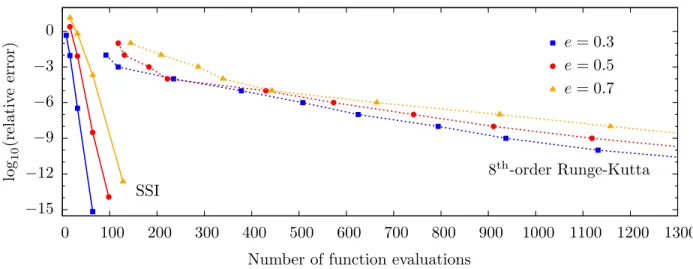
Figure 2.1: Efficiency of spectral source integration in comparison to ODE integration. The convergence of normalization constants C+ with l = 2, m = 2, n = 0 is shown for various eccentricities in orbits withp= 10. The ODE integration uses the Runge-Kutta-Prince-Dormand 7(8) routine rk8pd of the GNU Scientific Library (GSL) [97].
periodic motion is divided into equally spaced steps ∆χ = 2π/N, the integrand is discretely sampled, and the integral is replaced with the sum
C±= Ωr
N W
N−1 X
j=0
dtp
dχ E¯
±[t(χj)]einΩrt(χj). (2.62)
It is an open question whether there is another parametrization of the orbit that yields even faster conver-gence.
The benefit of SSI is shown clearly in Fig. 2.1, which describes the accuracy reached in computing a normalization coefficient (C220+ ) as a function of the number of source term evaluations, which serves as a proxy for computational load. SSI is compared to an ODE integration using an 8th order Runge-Kutta routine. SSI has exponentially converging accuracy with increases in function calls (i.e., increases inN). In contrast, the Runge-Kutta routine, with its algebraic convergence, struggles to reach high accuracies.
the energy fluxhE˙iand angular momentum fluxhL˙iare given by [74]
hE˙i=X lmn
ω2 mn 64π
(l+ 2)! (l−2)! |C
+ lmn|2+
|Clmn|− 2
, (2.63)
hL˙i=X lmn
m ωmn 64π
(l+ 2)! (l−2)! |C
+
lmn|2+|Clmn|− 2
CHAPTER 3: Lorenz gauge metric perturbations
The work discussed in this chapter is largely drawn from Refs. [65, 72, 73].
Section 3.1: Tensor-spherical-harmonic modes in Lorenz gauge
To calculate the gravitational self-force, the MP will be calculated in Lorenz gauge because regularization of the retarded field is straightforward in this gauge. As mentioned, the Lorenz gauge metric perturbation satisfies the following condition
∇µp¯µν = 0. (3.1)
This condition simplifies Eqn. (2.14) to the following [56]
42¯p
µν+ 2Rα βµ νp¯αβ=−16πTµν. (3.2)
This is a system of 10 coupled linear hyperbolic partial differential equations for the components of ¯pµν. Applying the tensor-spherical-harmonic projections of Eqn. (2.16) to Eqn. (3.2) yields coupled sets of field equations in t and r for the MP amplitudes. Eqn. (3.1) provides a set of Lorenz gauge conditions on the amplitudes. The seven even-parity and three odd-parity Lorenz gauge field equations are well-posed hyperbolic systems, but the Lorenz gauge conditions (three even parity and one odd-parity) force constraints on the initial data. These unconstrained field equations, along with the Bianchi identities, ensure that the gauge conditions, if fixed initially, are satisfied subsequently. The unconstrained equations are presented first, and then modifiedconstrained systems are introduced. Equations in this subsection are in time-domain form. In what follows alllandmindices on MP and source amplitudes are suppressed for brevity unless otherwise noted.
The seven even-parity unconstrained Lorenz gauge equations are
2htt+2(r−4M)f
r2 ∂rhtt+ 4M f
r2 ∂thtr+
2M(3M−2r)f2
r4 hrr
+4M f 2
r3 K+ 2(M2
−r2f)
−2λr2f
r4 htt=−f Q rr
−f2Q[−f3Qtt,
2htr+2f 2
r ∂rhtr+
2M f
r2 ∂thrr+ 2M
r2f∂thtt+
4(λ+ 1)f r3 jt−
4(M−r)2+ 2λr2f
r4 htr= 2f Q tr,
2hrr+ 2f
r ∂rhrr+
4M
r2f∂thtr+
2M(3M −2r)
r4f2 htt+
4(r−3M)
r3 K
+8(λ+ 1)f
r3 jr+
2(r−M)(7M−3r)−2λr2f
r4 hrr =Q
[