ENHANCED 3D CAPTURE FOR ROOM-SIZED DYNAMIC SCENES WITH COMMODITY DEPTH CAMERAS
Mingsong Dou
A dissertation submitted to the faculty of the University of North Carolina at Chapel Hill in partial fulfillment of the requirements for the degree of Doctor of Philosophy in the
Department of Computer Science.
Chapel Hill 2015
ABSTRACT
MINGSONG DOU: ENHANCED 3D CAPTURE FOR ROOM-SIZED DYNAMIC SCENES WITH COMMODITY DEPTH CAMERAS.
(Under the direction of Henry Fuchs .)
3D reconstruction of dynamic scenes can find many applications in areas such as virtu-al/augmented reality, 3D telepresence and 3D animation, while it is challenging to achieve a complete and high quality reconstruction due to the sensor noise and occlusions in the scene. This dissertation demonstrates our efforts toward building a 3D capture system for room-sized dynamic environments. A key observation is that reconstruction insufficiency (e.g., incom-pleteness and noise) can be mitigated by accumulating data from multiple frames. In dynamic environments, dropouts in 3D reconstruction generally do not consistently appear in the same locations. Thus, accumulation of the captured 3D data over time can fill in the missing frag-ments. Reconstruction noise is reduced as well.
The first piece of the system builds 3D models for room-scale static scenes with one hand-held depth sensor, where we use plane features, in addition to image salient points, for robust pairwise matching and bundle adjustment over the whole data sequence.
nonrigid bundle adjustment algorithm to simultaneously optimize for the final mesh and the deformation parameters of every frame.
Finally, we integrate static scanning and nonrigid matching into a reconstruction system for room-sized dynamic environments, where we prescan the static parts of the scene and perform data accumulation for dynamic parts. Both rigid and nonrigid motions of objects are tracked in a unified framework, and close contacts between objects are also handled.
TABLE OF CONTENTS
LIST OF FIGURES. . . ix
LIST OF TABLES . . . xi
CHAPTER 1: Introduction . . . .1
1.1 Challenges and Opportunities . . . .4
1.2 Thesis approach and overview . . . .6
1.3 Related work. . . .9
CHAPTER 2: Static Scene Reconstruction . . . 11
2.1 Other Related Work . . . 14
2.2 System Overview . . . 15
2.3 Planar Surface Extraction from Depth Map . . . 16
2.4 Robust Pair-wise Matching . . . 19
2.4.1 Plane Matching Hypothesis . . . 19
2.4.2 RANSAC on one plane matching hypothesis and the feature match set . . . 22
2.5 Bundle Adjustment of Points and Planes. . . 26
2.5.1 Problem Statement . . . 27
2.5.2 Cost Function . . . 27
2.6 Experiments . . . 31
2.6.1 Comparison to Structure from Motion (SfM) algorithms . . . 32
2.6.3 Comparison to ICP with global error mitigation. . . 33
2.6.4 Quantitative measurement of errors . . . 34
2.6.5 Running times . . . 35
2.7 Discussion . . . 35
CHAPTER 3: Nonrigid Alignment . . . 38
3.1 Nonrigid Alignment in Literature . . . 38
3.2 Nonrigid Alignment Problem . . . 40
3.3 Embedded Deformation Model. . . 41
3.4 Directional Distance Function and Measurement of surface alignment . . . 44
3.5 Color Consistency . . . 46
3.6 Comparison . . . 47
CHAPTER 4: Dynamic Surface Reconstruction . . . 49
4.1 Related work. . . 49
4.2 Scanning Dynamic Objects . . . 51
4.2.1 DDF Transformation from Target to Reference . . . 53
4.2.2 Fusion of multiple DDFs . . . 55
4.3 Dynamic Surface Tracking . . . 57
4.3.1 Tracking Surfaces with Isometric deformations . . . 57
4.4 Experimental Results . . . 58
4.4.1 Scanning . . . 59
4.5 Discussion . . . 62
4.5.1 Limitations of the System . . . 62
CHAPTER 5: Dynamic Surface Recontruction with a Single Depth Sensor . . . 65
5.1 Other Related Work . . . 68
5.2 Triangular Mesh Surface Model . . . 69
5.3 Extracting Partial Scans . . . 69
5.4 Coarse Scan Alignment . . . 72
5.5 Error Redistribution . . . 72
5.6 Dense Nonrigid Bundle Adjustment . . . 74
5.6.1 Deformation Terms . . . 75
5.6.2 Surface Regularization Terms . . . 76
5.6.3 Solving . . . 76
5.7 Experiments . . . 79
5.7.1 Implementation details . . . 79
5.7.2 Comparison with KinectFusion . . . 82
5.7.3 Comparison with 3D Self-portraits . . . 84
5.7.4 Synthetic sequence . . . 84
5.7.5 Scanned example . . . 86
5.8 Discussions . . . 86
CHAPTER 6: Room-sized Dynamic Scene Reconstruction . . . 89
6.2 Room-sized Dynamic Scene Reconstruction . . . 92
6.2.1 Room Scanning and Segmentation . . . 93
6.2.2 Unified Tracking Algorithm . . . 94
6.2.3 System Pipeline . . . 99
6.3 System Calibration . . . 104
6.4 Experiments . . . 106
6.4.1 Results . . . 107
6.5 Discussions . . . 107
CHAPTER 7: Conclusions . . . 109
7.1 Algorithmic Contributions . . . 110
7.1.1 Bundle Adjustment of Points and Planes . . . 110
7.1.2 Nonrigid Alignment Algorithm . . . 111
7.1.3 Dense Nonrigid Bundle Adjustment. . . 111
7.2 Developed systems in the disseration . . . 111
7.2.1 Indoor Static Environment Scanning System. . . 112
7.2.2 Dynamic Object Scanning and Tracking System . . . 112
7.2.3 Dynamic Object Scanning System with One Single Depth Sensor. . . 112
APPENDIX A: DDF CALCULATION PSEUDO-CODE . . . 114
LIST OF FIGURES
1.1 3D Medical Environment Reconstruction . . . .2
1.2 3D Medical Environment Reconstruction . . . .3
1.3 Room-sized reconstruction for a dynamic scene . . . .4
1.4 Data accumulation for dynamic objects . . . .5
2.1 Static Scanning Results . . . 13
2.2 Plane Extraction . . . 17
2.3 Extracted Planes . . . 18
2.4 Robust pairwise matching with both planes and features . . . 20
2.5 Distance measurement for plane segments . . . 24
2.6 Refined Match Sets . . . 26
2.7 Comparison . . . 37
3.1 Alignment Comparison of various algorithms . . . 48
4.1 Dynamic Object Scanning. . . 50
4.2 Scanning System Pipeline . . . 51
4.3 Fusing two 2D truncated signed distance fields . . . 55
4.4 Scanning Errors . . . 59
4.5 Intermediate Scans. . . 60
4.6 Scanning Results . . . 61
5.1 Teaser Image . . . 66
5.2 Scanning Pipeline. . . 70
5.3 Scanning a person with slight deformation . . . 77
5.4 Bundle Adjustment Residuals . . . 78
5.5 Example Results of Bundle Adjustment . . . 79
5.6 Bundle adjustment iterations . . . 80
5.7 KinectFusion with nonrigid alignment . . . 81
5.8 Static Scanning . . . 82
5.9 Comparison with 3D Self-Portraits . . . 83
5.10 Alignment error in Saskia dataset . . . 85
5.11 Scanning Results . . . 87
6.1 Room-sized Dynamic Scene Reconstruction. . . 90
6.2 Scanned Room Model and Scene Segmentation . . . 91
6.3 Various Intersection Situations . . . 97
6.4 Backward Deformation Graph Generation . . . 99
6.5 Results of tracking one person folding arms . . . 102
6.6 Results of tracking one person sitting on a chair . . . 103
6.7 Depth bias v.s. depth . . . 104
6.8 Tracking two persons where severe occlusion happens . . . 105
LIST OF TABLES
CHAPTER 1: Introduction
Reconstructing a scene digitally, or capturing its 3D geometric model, has been one of the most challenging and fundamental problems in Computer Vision since its emergence, and high quality 3D reconstruction is essential for many potential but yet unrealized applications in virtual and augmented reality. For example, virtual reality applications, such as surgical train-ing programs and science demonstration, could continually record raw imagery (and sound) inside operating rooms; when noteworthy events occur (e.g., a difficult trauma surgery case), reconstruction and subsequent annotation would be triggered, to generate an immersive virtual presence training module. To be effective, such modules should encourage free navigation and user-selectable viewpoints and also have high reconstruction fidelity without any undesired artifacts. Figure 6.1 illustrates the above concept.
(A) 3D capture during medical procedure (B) immersive experience of the 3D reconstruction Figure 1.1: 3D Medical environment reconstruction for medical training. (A) Operating room is instrumented with various capture devices such as depth and pan-tilt-zoom cameras; medical personnel wear miniature cameras. (B) The procedure has been reconstructed in three dimen-sions and annotated (orange). A medical student (grey) experiences the reconstructed sequence immersively within a modern low-latency, wide-field-of-view head-worn display, navigating in space and time.
users right in front of the display), lack of 3D information of the scene prevents us from gen-erating proper views for all users. This early attempt motivated us to work on 3D room-sized reconstruction.
The above applications demand sufficiently accurate 3D reconstruction to enable unencum-bered and seamless immersion into the reconstructed environment. In addition, most activities of interest involve not just static scenes, but also moving objects and people which are much more difficult to reconstruct. Thus, in this dissertation we focus our research on a dynamic 3D-plus-time reconstruction of an actively evolving scene in indoor environment.
Figure 1.2: Illustration of concept of 3D telepresence. Every location is reconstructed in 3D and every person gets a custom view of the remote scenes from the 3D display. The wall on the right side is instrumented with autostereoscopic displays, through which people in the local room see the combination of two remote rooms.
scene reconstruction can impact society profoundly. It could influence the way we share infor-mation. Instead of sharing photos on social media, people could share recorded 3D videos that can be immersively experienced. It could also change the way we interact with other people and the environment, via applications such as immersive virtual visits to interesting locations and virtual attendance at events such as concerts or a class.
Figure 1.3: Room-sized reconstruction for a dynamic scene by performing data accumulation and background prescan. Top: input depth points from 10 Kinects; Bottom: enhanced recon-struction. The rendering from the perspective of the man standing at right is shown on the right. Note the low quality on the input data despite there being 10 cameras. Note also we did not shake the sensors to reduce some level of sensor interference (Maimone and Fuchs, 2012; Butler et al., 2012).
sensors (i.e., Kinect) to achieve high quality reconstruction for room-sized dynamic scenes.
1.1 Challenges and Opportunities
Figure 1.4: Data accumulation for a person turning around in front of depth sensors. Surfaces after fusing 1, 5, 50, and 150 frames of data.
Kinect sensor has difficulty reconstructing low or high reflective surfaces. In addition, incom-pleteness is also caused by occlusion, which includes self-occlusion as well as inter-occlusion of objects. Yet another undesired artifact comes from the significant amount of noise in the data from depth sensors (Maimone and Fuchs, 2011; Beck et al., 2013).
be accumulated, they must be aligned spatially, which requires tracking corresponding surface fragments accurately over time. An insufficient alignment will lead to smoothing of surface de-tails and geometric features. To use this data accumulation concept in real-world applications, we must deal with the following challenges:
• Nonrigid movement. In many cases, especially when processing deformable geometry such as human bodies, a nonrigid alignment algorithm must be employed. An ideal alignment algorithm should be robust to data dropouts on surfaces and work for general surfaces (i.e., without assumptions on the surface shape).
• Dynamic topology. In real scenarios, there are many topology changes in the geometry of the scene caused by people and objects engaging contact (e.g., shaking hands, sitting on a chair).
• Drift. Even for rigid alignment of non-deformable objects, drift occurs when accumu-lating a sequence of geometric data over a period of time and thus over a number of capture events (frames). As alignment error accumulates, scanned surfaces do not close seamlessly.
1.2 Thesis approach and overview
In this dissertation, we developed several systems that employ the data accumulation strat-egy to enhance surface reconstruction for indoor dynamic environment while tackling afore-mentioned challenges. Specifically,
data from one single hand-held depth sensor.
• We also perform data accumulation for the dynamic part of the scene via nonrigidly aligning data to the same reference pose. The data either come from the depth sensors mounted over the walls or from a single depth sensor (hand-held or fixed). Deforming the accumulated model to align the data at every frame results with enhanced dense reconstruction.
• We combine static pre-scanning with nonrigid accumulation, leading to a dense recon-struction system for a room-sized dynamic scene. In addition, we estimate the rigid movements for static objects (e.g., chairs, tables) and handle close contact between ob-jects.
We will introduce the static scanning in Chapter 2, the dynamic object scanning with multiple depth sensors in Chapter 4, the nonrigid surface reconstruction with one single depth sensor in Chapter 5, and the combination of static pre-scanning and nonrigid accumulation for room-sized dynamic reconstruction in Chapter 6. We will conclude the dissertation in Chapter 7 with summarizing our contribution and listing future work.
Drift is a ubiquitous problem when aligning a sequence of data together, happening in both rigid and nonrigid cases. For static scanning, we incorporate plane features into the bun-dle adjustment framework to mitigate the error over the whole data sequence, in observance of planes being the dominant feature for the indoor environment. For dynamic surface re-construction from a single depth camera, we developed a dense nonrigid bundle adjustment technique which simultaneously optimize both the dense geometry and deformation parame-ter. The new bundle adjustment technique takes dense partial structure as input and outputs the optimal fused surface and nonrigid motion. For the data accumulation from multiple units of depth sensors, since the data is relative complete at a frame (compared with the case of a single depth sensor), we take a computationally less intense algorithm. We estimate the deformation of the currently accumulated model to the current data observation and build the point-to-point correspondence, from which a backward deformation that deforms data to the model is esti-mated. Then we fuse the current data into the model and repeat the above procedures. This strategy would be proven effective in Chapter 4.
Note that we focus on reconstruction quality rather than on real-time processing in this dis-sertation,i.e., the data are captured in real time while being processed offline. Such techniques are still valuable as many potential applications do not require real-time reconstruction but have stringent reconstruction quality requirement. It is the case with the aforementioned medi-cal and surgimedi-cal training, where high quality reconstruction and faithful presentation of delicate and intricate 3D manipulations is paramount. Furthermore, with continuous advances in com-puting power and GPU-enabled parallelization, it can be reasonably expected that the proposed techniques will be applied to real-time situations in the near future, allowing telepresence-type interactions.
1.3 Related work
We will give a brief summary of work on 3D reconstruction here. More related work for each system component is provided at following chapters. Traditional 3D reconstruction al-gorithms, including stereo vision (Scharstein and Szeliski, 2002) and multi-view vision (Seitz et al., 2006) algorithms, rely on color cameras and have difficulties when processing texture-less surfaces. Recent consumer-targeted depth sensors, such as the Microsoft Kinect and Intel 3D perception sensor, dramatically changed the field due to their high performance-price ratio. These sensors either employ the infrared projector and camera system or time-of-flight tech-nique and are able to give real-time reliable depth maps even for textureless areas. These lead to static reconstruction approaches such as KinectFusion (Newcombe et al., 2011; Izadi et al., 2011), commercial softwares such as ReconstructMe2 and Matterport3.
The work of using Kinects for realtime reconstruction application with light-weight pro-cessing on the depth maps include (Beck et al., 2013; Kuster et al., 2011), where the recon-struction is far from complete and often has a high level of noise. Other reconrecon-struction systems that require highly controlled environment or employ expensive hardware include USC Light Stage (Vlasic et al., 2009; Ghosh et al., 2011) and ETH Blue-C project (Gross et al., 2003).
CHAPTER 2: Static Scene Reconstruction
In this chapter, we introduce our 3D scanning system for room-sized static scenes using one depth sensor/RGB-D camera (e.g., Microsoft Kinect). RGB-D cameras are new addition to vi-sion sensors for 3D reconstruction, which output RGB images and corresponding depth images at video frame rate. Recent approaches demonstrated the use of a single hand-held RGB-D camera for scanning an indoor environment (Henry et al., 2010; Izadi et al., 2011; Newcombe et al., 2011; Neumann et al., 2011; Lieberknecht et al., 2011) and even large scenes (Chen et al., 2013; Nießner et al., 2013; Zhou et al., 2013).
These algorithms roughly fall into two major categories: (1) point cloud based registration such as Iterative Closest Point (ICP) and (2) visual feature based Structure from Motion (SfM). KinectFusion system (Izadi et al., 2011; Newcombe et al., 2011) utilizes ICP to align one frame’s structure with previously captured data. While achieving subpixel accuracy in certain environment settings (e.g., table-sized scene), the major drawback is that ICP relies only on distinctive geometric information and would be confused when scanning geometrically smooth region (e.g., a wall), leading todrift.
algorithms are expected to fail in challenging cases where a scene has very few image and geometry salient features.
However, we notice that additional high level contraints exist in the depth channel. As shown in Fig. 2.4, although there is no image feature correspondence detected around the ceil-ing, the two frames can still be well aligned by extracting planes from the depth map and searching for the correct plane matches. By combining high-level depth information and low-level image salient features, our system handles well previously mentioned challenging situa-tions, which cannot be solved alone by ICP or SfM.
In the SfM literature, the final step is usually global error mitigation through bundle adjust-ment (BA) (Snavely et al., 2007, 2006; Crandall et al., 2011). This global adjustadjust-ment step is crucial for building a model for a large scene such as an entire room. However, as shown in Chapter 5, it takes huge efforts (e.g., computation power) to directly incorporate dense point cloud into the BA framework due to implicit point association. Instead, this chapter proposes to use a compact planar representation of dense point clouds and integrate it into the traditional BA formulation.
To summarize, the major contributions of the indoor scanning system introduced in this chapter include:
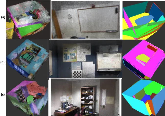
Figure 2.1: Results of the scanning system on datasets (a)Rm. FB220, (b)Rm. SN277 and (c)Rm. SN353. Accumulated point clouds (colors are added to distinguish points from different planes), zoomed view, and planes resulted from our algorithm are shown from left to right.
• Second, a novel formulation for incorporating plane correspondences (in addition to vi-sual feature correspondence) into the bundle adjustment framework. Planes are more compact than points and have clear associations across frames. This bundle adjustment step eliminates the drift problem that hurts KinectFusion.
• In addition, our proposed algorithm results in a piecewise planar representation for pla-nar parts of the scene. Such compact representation of the scene can be deployed for applications such as noise reduction, data compression, segmentation, etc.
represen-tation is most natural for man-made indoor environments, due to the dominant existence of planar surfaces, such as walls, floors, etc.
We evaluate our approach on several real world indoor datasets. Some have a lot of texture-less regions, which confuse SfM algorithms; some also have areas with significant geometrical ambiguity, such as large pieces of walls, which confuse ICP algorithms. By combining low level appearance features and high level geometric primitives, our algorithm handles these challenges well and significantly improves the reconstruction results.
2.1 Other Related Work
our method is that we perform bundle adjustment on both image features and planes.
2.2 System Overview
To build a complete room model, a sequence of RGB-D images is captured from a hand-held depth sensor. The camera intrinsics are pre-calibrated, thus we only need to estimate the camera poses (extrinsics, namely camera rotations and translations) to reconstruct the room. Note that depth calibration (detailed in Chapter 6) helps the reconstruction quality for large scene.
For every frame in the sequence, we extract SIFT features from RGB color image and planar patches from the depth maps (detailed in Section 2.3). The corresponding 3D coordinate for each image feature point is calculated under its camera coordinate system, given that the depth value at its image location is known. We call these 3D points originating from image features simply as “features” or “points” in order to differentiate them from planes extracted from depth maps. We remove features that are located at discontinuity regions in the depth map as their depth values are typically inaccurate.
are automatically selected during the matching procedure. When a new frame comes, it is only matched against previous key frames and a few neighboring frames.
Finally, we run a bundle adjustment algorithm on all the matched features and planes from all pairs of the matched frames to optimize camera poses globally. The bundle adjustment al-gorithm is carried out directly in 3D space instead of 2D image space thanks to the 3D location information computed from the depth channel. Different from traditional bundle adjustment, planes provide strong constraints for camera pose estimation in indoor environment. This ex-tended bundle adjustment algorithm is introduced in Section 5.6. We evaluate the proposed system with plane constraints in Section 6.4 qualitatively and quantitatively and demonstrate significant improvement over state-of-the-art reconstruction algorithms in real world indoor datasets.
2.3 Planar Surface Extraction from Depth Map
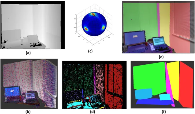
Given the camera intrinsics, a depth map can be transformed to a point cloud, and vice versa. Therefore we use these two terms interchangeably. In the literature of plane extraction from point cloud, region growing (Poppinga et al., 2008) and voting (Borrmann et al., 2011) are two popular techniques. Region growing algorithms scatter some initial seeds over the image, and gradually merge neighboring pixels belonging to the same plane. The voting algorithms transform all points into plane parameter space. The peaks in the parameter space correspond to the consensus planes in the original space. A plane in 3D space is represented as
Figure 2.2: Planar surface extraction via voting in plane parameter space. (a) input depth map; (b) normal vectors of local planes at each pixel; (c) votes in the plane parameter space; (d) pixels voting for the same peaks; (e) final plane labels; (c) the plane segments in 3D
wheren = {nx, ny, nz}is the plane normal—a 3D unit vector; dis the distance of the plane
to the camera optical center. We force the plane normal point away from the origin, resulting a positived. From now on, we letP =hn, di, representing a plane under its individual camera coordinate system for that frame.
Figure 2.3: Example of extracted planes.
hρ, θ, φiis used for plane voting,i.e.,
θ= cos−1nz
φ= tan−1 ny
nx
ρ=d,
(2.1)
examples of extracted planes are shown in Figure. 2.3.
2.4 Robust Pair-wise Matching
Given the detected planes and features for two frames, next we find the matched features and matched planes if any. The geometric transformation that aligns these two frames is also estimated accordingly. Conventionally, we represent the transformation as a rotation matrixR
and a translation vectorT, satisfying
Xr =RXl+T,
where Xl and Xr are 3D points under two camera coordinate systems respectively (left and right). To reduce the searching space of matched planes and features, the initial feature and plane match set are found before being refined with RANSAC.
2.4.1 Plane Matching Hypothesis
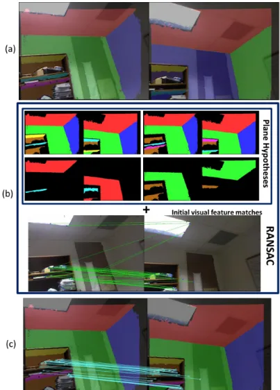
Figure 2.4: Robust Pairwise Matching of Both Planes and Features. (a) two input frames and detected planes. (b) four plane matching hypotheses are shown on top (same color indicates a plane match), and the initial feature matches are shown on bottom. (c) matched features and planes after RANSANC.
the following RANSAC stage is able to find a unique solution.
Finding two matched plane subsets is equivalent to finding a rotation matrix that rotates the plane normals in one set to match the plane normals in the other set. Theoretically, a brute force search on the rotation matrix space is a possible solution. That is, we apply all possible rotation matrices on the planes of one frame, and find a subset of planes in this frame that have corresponding planes with similar plane normals and appearance in the other frame.
However, the above brute force algorithm is not practical as it searches a 3D space for the rotation matrix. Similar to (Pathak et al., 2009), we take advantage of the fact that a rotation matrix can be decomposed into a rotation axis and a rotation angle about the axis. Specifically, we repeat the following procedures:
1. Pick one pair of planeshPl
i,Pir0ithat have similar appearance from two frames, and find a rotation matrixRthat rotates normal vectorni toni0, i.e.,Rni =ni0.
2. ApplyRon all the planes in the first frame. By now,Pl
i andPir0’s normals are aligned, but most likely not any other planes in the two views.
3. Rotate the planes of the first frame about axis Rni to find their matched planes with
similar plane normals and appearance in the second frame. In this way, we search along only one dimension—the rotation angle about axisRni.
Note that using d in plane parameter as an extra constraint will give better plane matching hypotheses but also increase the search space (6 DOF).
For each plane segment, we calculate a hue-saturation joint histogram hHS to represent
appearance similarity of the two planes is defined as the overlapping area of their histograms, i.e.,
X
i
min(hHS1 (i),hHS2 (i)) +X
i
min(hI1(i),hI2(i)).
2.4.2 RANSAC on one plane matching hypothesis and the feature match set
The initial feature match set might contain spurious pairs, as might a plane matching hy-pothesis. We use RANSAC to find the underlying geometric transformation between two frames and refine the match sets. When a feature or plane pair fits a candidate transforma-tion, it supports this transformation (details are given later). RANSAC returns a transformation that collects most supports from match sets. Note RANSAC is extended to take both the fea-ture match set and plane match set as input. Since Section 2.4.1 might return multiple plane matching hypotheses, we run RANSAC multiple times on every plane matching hypothesis together with initial feature match set. Within multiple transformations returned by RANSAC, again we pick the one that collects most supports.
Randomly sample matched pairs
different normal direction than the vector connecting the two feature points. Our randomly sampled match subsets are evenly distributed over the above four cases—three planes, three features, two planes with one feature, and two features with one plane.
Calculating the transformation from pairs of matches
Inside each loop of RANSAC, the transformation needs to be calculated from the randomly sampled matches (the seeds). We consider a general case, where there aren pairs of matched planes S = {hPl
i,Pir0i}, and m pairs of matched features T = {hfil,fir0i}. The upper-index l and r indicates which frame the data belong to, and we will ignore them whenever it does not cause confusions. A transformation hR, Ti is estimated to minimize the overall distance between matched items. That is,
min X
hPl i,Pir0i∈S
D2pln(Q(R, T,Pl i),P
r i0) +
X
hfl i,fir0i∈T
D2pt(Rfil+T,fir0). (2.2)
whereQ(·)applies transformationhR, TitoPl
i and is detailed later, whileDpln(·)andDpt(·)
Figure 2.5: The closeness on planes parameters shown in (a) does not equal to the closeness of plane segments shown in (b). The solid line segments denote the plane segments, ando is the origin of the world coordinate. In (b), even though each pair of matched planes have much larger difference on the origin-to-plane distanced, they are better aligned comparing with (a).
Distance between plane segments
Instead of measuring Euclidean distance between plane parameters, we measure the dis-tances from the boundary points (convex hull) of one plane segment to its matched plane. Ideally, we could use the sum of the point-to-plane distances from all points in one plane seg-ment to the other plane, since these points are the direct observations of a plane. However it is computationally more expensive given the number of points in a plane segment. It can be proven the convex-hull-to-plane distance is the upper-bound of the sum of point-to-plane distances1.
1Each observed pointpassigned to a plane could be represented by a linear combination of the convex hull vertices
{vi}, i.e.,p=Picivi+; wherePici= 1andaccounts for the fact that the pointpmight not lie exactly on
the fitted plane. Since the point-to-plane distance is a convex function, the weighted sum of convex-hull-vertex-to-plane distances is statistically the upper-bound of the distance from an observed point to the world plane. Taking all the points associated with one plane into consideration, the sum of squared point-to-plane distances (upper-bound) iscP
iwiD
2(v
Let’s assume we are measuring the distance between two plane segments {Pl
i,Pir0}under the transformationhR, Ti. The the convex hull vertices of two plane segments are{vl
i,k} K1 k=1
and{vr
i0,k}Kk=12 respectively. As shown in (Pathak et al., 2010), after applying the transformation hR, Ti to plane Pl
i, its plane parameter becomes hRni, di + nTi RTTi, and its convex hull
vertices becomes {Rvi,k +T}Kk=11 . Then the distance between plane segments in Eq. 2.2 is defined as,
D2pln =
K1 X
i=1
wi,kknTi0Rvi,k+nTi0T −di0k22+ K2 X
i=1
wi0,kknTiRTvi0,k−nTi RTT −dik22. (2.3)
The first term in the right side of the equation measures the perpendicular distance from the transformed convex hull vertices on the first plane to the second plane, while the second term measures the distance between the vertices of the second plane and the transformed first plane. Each point-to-plane distance is given a weightwi,k, satisfying
P
kwi,k = 1. Because vertices
on the convex hull are not a uniform sample of the plane boundary, larger weights are given to vertices further away from their neighboring vertices.
Find the supporting pairs and choose the best transformation
For each transformation candidate, we count the support from the match sets. A pair of points will cast a constant vote value cpt if their distance is closer than pt, while a pair of
planes cast vote valuecpln if their distance defined in Eq. 2.3 is less than pln and two plane
segments overlap after transforming one plane’s segment to the other plane’s image space. That is, only when a pair of planes are close enough and have overlap under one transformation, we
Figure 2.6: Two examples of point and plane match sets after refinement.
say they fit the transformation. In our experiment, plane pairs carry more weight than point pairs. Examples of the refined match set are shown in Figure 2.6.
2.5 Bundle Adjustment of Points and Planes
After performing the above robust pairwise matching algorithm over the whole RGB-D sequence, we have a large number of feature/plane match sets, and groups of matched fea-tures/planes are linked together according to . A set of linked features {fki}i∈Ck is called a
feature track, corresponding to the same 3D pointpk in a world coordinate system. The
no-tationfi
krepresents a 3D feature point in thek-th visual feature track from thei-th frame, and
Ck is the set of frame indices where all the indexed frames have feature corresponding to the
found. Each plane track is composed of a set of linked planes {Pi
j}i∈Dj from various frames
corresponding to the same world planeQj. The notationPjirepresents a plane in thej-th plane
track and extracted fromi-th frame, whileDj is the set of frame indices where all the indexed
frames have the extracted planes corresponding to the world plane Qj. From now on, we
al-ways useias the index of frames, j as the index of the plane track or its corresponding plane in the world space, andk as the index of the visual feature track or its corresponding point in the world space.
2.5.1 Problem Statement
GivenM plane tracks{{Pi j}i∈Dj}
M
j=1, andK feature tracks{{fki}i∈Ck}
K
k=1, which are rep-resented under their own camera spaces, the bundle adjustment problem is to simultaneously optimize the camera poses {Ri, Ti}Ni=1 for N frames in the sequence, the plane parameters {nj, dj}Mj=1 for M planes{Qj}in the world, andK point locations{pk}Kk=1 in the world. As a usual practice, the camera pose is represented by rotation matrix R and a 3D translation vectorT, which transform a pointXwld in world space to the camera space coordinateXcvia Xc=RXwld+T.
2.5.2 Cost Function
c Npln
X
{i,j|i∈Dj}
cijDpln2 Q(Ri, Ti,Qj),Pji
+
1−c Npt
X
{i,k|i∈Ck}
D2pt Q(Ri, Ti,pk),fki
,
(2.4)
where Dpln(·) measures the distance between a detected plane and the world plane, while
Dpt(·)measures the distance between an observed feature and a world point. Q(·)transforms
a point or a plane in the world space to a certain camera space given the camera pose. Constant
c weights the effects of plane tracks against feature tracks; Npln and Npt are the number of planes in all plane tracks and the number of points in all feature tracks respectively. cij is the weight on the plane in the plane track and equals to the number of associated pixels in a plane divided by the average number of pixels among planes in all plane tracks.
Again we use the Euclidean distance to measureDpt, i.e.,
Dpt2 (Q(Ri, Ti,pk),fki) =kRipk+Ti−fkik
2 2.
For distance between a detected plane and a world plane, as in Eq. 2.3, we measure the convex-hull-to-plane distance, i.e.,
D2pln Q(Ri, Ti,Qj),Pji
=X
h
wj,hi knTjRTi vij,h−nTjRTi Ti−djk22,
where {vi
parameters ofQj. Putting everything together, we have the cost function,
c Npln
X
{i,j,h|i∈Dj}
cijwj,hi knTjRTi vj,hi −nTjRiTTi−djk22+
1−c Npt
X
{i,k|i∈Ck}
kRipk+Ti−fkik22.
(2.5)
Note that the camera pose for the very first camera is fixed at the origin with an identity rotation matrix in the above function.
Statistically speaking, the noise on observed points comes from variant independent factors, for example, errors from the 2D SIFT detector, depth map, camera calibration, thus we assume it is normally distributed based on Central Limit Theory. Hence, L2 norm is used to measure the error of an observed feature in the above cost function. As to the measurement of the error on a plane segment, we use the convex-hull-to-plane distance as a compromise since it is computationally prohibitive to use the sum of the point-to-plane distances given the number of points. As stated earlier, this convex-hull-to-plane distance is statistically the upper-bound of the error of the points on the plane segment. Since this error (or noise) also comes from various independent factors, we assume it is normally distributed and L2 norm is used.
Initialization and optimization
#features #matched #feature #plane #planes dataset #frames per frame features tracks tracks in tracks
SN353 228/191 328 143 6066 83/52 1179/916 SN277 381/350 497 129 10695 155/72 1896/1520 FB220 360/280 137 46 3357 138/64 1516/1232 Lab 180/180 694 267 10636 85/46 1236/858
Table 2.1: Statistics on four datasets. Under column “#frames”, the number of frames in the sequence is recorded before the slash, while the number of frames registered with others is shown after the slash. The third and fourth column give the average number of all detected features and matched features respectively. Column “#plane tracks” gives the number of the detected plane tracks provided to BA and also the number of planes tracks after refinement in BA. Column “#planes in tracks” gives the total number of planes in all tracks before and after BA.
sets of unknowns, only the camera poses need to be initialized. The initial parameters for the world planes and world points are estimated from their corresponding tracks with the given camera poses. The camera poses are initialized one by one with the pairwise matching results.
Plane track refinement
Since we do not match every possible frame pair, some large planes tend to have several disjoint plane tracks instead of one complete track. These plane tracks need to be merged together. We compute the plane distance between estimated planes in the world space returned by bundle adjustment according to Eq. 2.3; if some of them are closely located, we merge them into one plane and also merge their plane tracks accordingly. Moreover, we delete a detected plane from its plane track if its distance to the corresponding world plane is beyond a threshold
2.6 Experiments
We evaluate our algorithm on four datasets of indoor office settings captured in real-world environment: SN353, SN277, FB220 and LAB. All the datasets except “LAB” have consid-erably fewer visual features. Some statistics on the datasets when running our algorithm are shown on Table 2.1. In each data set, 200 to 500 frames of RGB-D data are captured with sig-nificant overlaps. Among four datasets, “FB220” is the most challenging one, since the num-ber of detected feature is dramatically fewer than others. On average, there are only around 10 matched points per matched frame pair (the number “46” shown under the forth column for “FB220” is the average number of the features in one frame that have matches in all other frames), which can hardly lead to robust registration (camera pose transformation between two frames) with traditional SfM methods. As shown in the second column of Table 2.1, some frames are not registered with others and thus abandoned. This is because: (1) a frame is only matched with key frames and some adjacent frames; (2) the white balance and gain of the RGB channel on Kinect is in “auto” mode and cannot be disabled with current drivers, so the appearance of objects (mainly walls and ceilings) across frames changes dramatically, espe-cially when pointing the camera towards a light (which explains why some ceiling parts in the following results disappear), leading to missing matches between frames.
dataset point proj error(cm) plane proj error(cm) zero angles(°) right angles(°) SN353 1.46±1.37 1.74±2.03 -0.60±2.95 89.97±2.14 SN277 2.01±1.83 1.68±1.58 -0.22±0.80 89.94±1.70 FB220 2.38±1.63 2.36±2.15 -1.17±2.41 89.96±2.42 Lab 1.91±1.77 1.91±1.66 -0.59±4.27 89.61±2.11
Table 2.2: The quantitative measurements of our algorithm. Inside each cell, the average error and the standard deviation are provided.
a volumetric method such as (Izadi et al., 2011; Newcombe et al., 2011) could be used to fuse all the depth map together given the camera poses.
2.6.1 Comparison to Structure from Motion (SfM) algorithms
To compare our method with state-of-the-art SfM algorithms, we ran Bundler (Snavely et al., 2007)(Snavely et al., 2006) on all datasets. Since camera poses from SfM are determined up to a scale, we need to the find this scale compared to the one used by the depth camera. SfM outputs a sparse point cloud which can be projected to image space to extract the depth values from the depth cameras. Hence by comparing the depth values from the depth camera and those from Bundler, we have the relative scale.
2.6.2 Comparison to ICP method
We compared our system with ICP algorithm (Henry et al., 2010). Since RGBD-ICP also uses visual features to constrain the planes from drifting along the plane surface direction arbitrarily, it achieved better result than Bundler. But our algorithm comfortably out-performed RGBD-ICP algorithm as shown in Fig. 2.7(b), since the error accumulation problem is not handled in RGBD-ICP, while we address that with our new bundle adjustment formu-lation. We also compared our system with KinectFusion(Izadi et al., 2011; Newcombe et al., 2011) which uses only the depth information to align one frame with previously accumulated data. And as expected, KinectFusion did not result in a reasonable output on our dataset either, due to its lack of constraints to handle the drifting in some frames with simple geometry struc-ture.Since our reconstruction input frames are temporally down-sampled from the original 30 fps hand-held Kinect streams, the adjacent frames normally have noticeable amount of camera pose differences. Hence, for RGBD-ICP and KinectFusion to work, a decent initial camera pose is required. The transformation returned by our robust pairwise matching algorithm in-troduced in Sec. 2.4 is used for camera pose initialization.
2.6.3 Comparison to ICP with global error mitigation
as in (Grisetti et al., 2007), we distribute the error over the graph by minimizing
X
(i,j)∈E
kRj←i−RjRTi k22+kTj←i−Tj+Rj←iTik22. (2.6)
As shown in Fig. 2.7(c), after distributing the accumulated error, ICP gives decent results. However, some details are not preserved as well as using our method. For example, the ceiling in “SN277” is distorted as shown in Fig. 2.7(c). Note that both ICP with and without error re-distribution have to use our robust pairwise matching algorithm with planes and features for initial registration, otherwise both ICP algorithms would fail frequently in texture-less regions.
2.6.4 Quantitative measurement of errors
2.6.5 Running times
Our single thread program takes 2.5 to 3 seconds to extract planes from one frame, another 1.5 seconds to extract SIFT features on a desktop PC with 3.0 CPU Hz. Depending on how many planes and features are in the frames, it takes up to a few seconds to finish one pairwise matching. In our four datasets, the pairwise matching on a whole sequence takes two to five hours. We do not perform incremental bundle adjustment, and instead we perform BA on all frames directly. Generally it takes less than fifty iterations to converge with the default param-eters of the chosen Levenberg-Marquardt solver (Lourakis, 2010). We run bundle adjustment and the plane track refinement repeatedly. The whole BA procedure takes 5 to 20 minutes on a dataset. We expect significant computation speed acceleration with optimized code or on parallel processing unit such as GPU. This remains one of the future directions of this research work.
2.7 Discussion
CHAPTER 3: Nonrigid Alignment
In the following chapters, we focus on the 3D reconstruction problem for dynamic objects. As introduced in Chapter 1, we take advantage of the dynamic properties of the object being captured by accumulating data from multiple frames, which requires nonrigidly aligning data across frames. In this chapter, we will introduce the nonrigid alignment algorithm which is the fundamental component for techniques proposed in following chapters.
3.1 Nonrigid Alignment in Literature
Another category of methods takes the indirect approach and estimates deformation param-eters instead. Some work (Gall et al., 2009; Vlasic et al., 2008; Ballan and Cortelazzo, 2008; De Aguiar et al., 2008; Wu et al., 2013; Schmidt et al., 2014) assumes the articulated surface structure and use the kinematic model (i.e., skeleton model) to parameterize the deformation. They typically need a manual skinning procedure, i.e., attach the pre-scanned surface (volume in case of (Schmidt et al., 2014)) to a skeleton structure or kinematic tree. The skeleton param-eters are then estimated by matching the skeleton-driven surface with the current observation, such as silhouettes. A later surface refinement stage is usually employed to reduce the artifacts on the deformed surface resulting from the coarse deformation model.
3.2 Nonrigid Alignment Problem
3.3 Embedded Deformation Model
In general, we will want to allow our meshes to deform, for example to allow our surface reconstruction to explain the data in a depth sequence. Our desire to keep our algorithm ag-nostic to object class led us to choose the embedded deformation (ED) model of Sumner et al. (2007) to parameterize the non-rigid deformations of a meshV. In this model, a set ofK “ED nodes” are uniformly sampled throughout the mesh at a set of fixed locations{gk}Kk=1 ⊆ R3 and neighboring ED nodes are connected to form a graph. Each vertexm is “skinned” to the ED nodes by a set of fixed weights{wmk}K
k=1 ⊆[0,1], where
wmk = (max(0,1−d(vm,gk)/dmax))2/wsum
with d(vm,gk) the geodesic distance between the two, dmax the distance of vm to its c
+1-th nearest ED node, and wsum1 the normalization weight. Note vm is only influenced by its c
nearest nodes (c = 4 in our experiments) since other nodes have weights 0. The weighted deformation of the vertices surrounding gk is parameterized by a local affine transformation Ak ∈R3×3 and translationtk ∈R3.
In addition, we follow Zeng et al. (2013); Li et al. (2013) in augmenting the deformation using a global rotationR ∈ SO(3) and translationT ∈R3. The precise location of vertexv
m
deformed using the parameter setG={R, T} ∪ {Ak,tk}Kk=1 is
ED(vm;G) = R K X
k=1
and its associated surface normal is (withbbxcc:=x/kxk):
ED⊥(nm;G) = R $$ K
X
k=1
wmkA−kTnm %%
. (3.2)
In addition, we allow the former functional to be applied to an entire mesh at a time to produce a deformed mesh
ED(V;G) :={ED(vm;G)}Mm=1.
In general, we will want to find parameters that either exactly or approximately satisfy some constraints (e.g. ED(vm;G)≈ pk ∈ R3), and thus encode these constraints softly in an
energy functionEcon(G),e.g.,
Econ(G) =kpk−ED(vm;G)k2.
In order to prevent this model from using its tremendous amount of flexibility to deform in unreasonable ways, we follow the standard practice of regularizing the deformation by aug-mentingE(G)with
Erot(G) =
K X
k=1
kATkAk−IkF + K X
k=1
(det(Ak)−1)2, (3.3)
that encourages local affine transformations to be rigid, and
Esmooth(G) =
K X
k=1
X
j∼k
that encourages neighboring affine transformations to be similar. For clarity, in later equations, we use
Ereg(G) =αErot(G) +Esmooth(G), (3.5)
whereα= 10in our experiments. In addition, rigidity is encouraged by penalizing the defor-mations at ED nodes,
Erigid(G) =
X
k
ρ(kAk−IkF) + X
k
ρ ktkk2
, (3.6)
whereρ(·)is a robustness kernel function.
To summarize, nonrigid alignment paramters are estimated for the deformation graph by solving,
min
G wregEreg(G) +wrigidErigid(G) +wconEcon(G) (3.7)
It is straightforward to minimize this energy using standard nonlinear least squares optimiza-tion (Sumner et al., 2007; Li et al., 2009). The third term Econ comes from the matched key
points of two surfaces, In our case, the key points are Lucas-Kanade corner points that are converted to 3D points from 2D image locations using their observed depth.
and color consistencyEclr(Section 3.5), transforming Equation 3.7 to
min
G wregEreg(G) +wrigidErigid(G) +wconEcon(G)
+wdns ptsEdns pts(G) +wclrEclr(G)
(3.8)
3.4 Directional Distance Function and Measurement of surface alignment
The matched key points in Sec. 3.3 are sparse features on the surface; their alignment does not represent the global surface alignment. Thus the dense alignment must be measured. Dif-ferent from Li et al. (2009) who iteratively estimates dense point correspondence, we represent the target surface as a distance field so that the surface alignment can be efficiently measured. At each voxel of this volume data, we record its distanceD(·) and directionP(·)to its clos-est point on the surface. This representation is an extension to the Signed Distance Function (SDF) (Curless and Levoy, 1996), and we call it the Directional Distance Function (DDF). Then, the energy function for dense point cloud alignment is defined by,
Edns pts(G) =
X
i
D(˜vi) 2
(3.9)
wherev˜i =ED(vi, G).
is identified either as pixels on a depth map that have depth discontinuity with their neighbors or the vertices on a triangular mesh that do not share its edge with other triangles.
P(·)in the Directional Distance Function is especially helpful when minimizing Eq. 6.3. Since the energy function is in least squares form, it can be efficiently solved via a gradi-ent descgradi-ent-like method (e.g. Gauss-Newton algorithm) as long as the Jacobian matrix J is provided. To solve this nonlinear least squares problem, we use the Levenberg-Marquardt al-gorithm (Madsen et al., 2004) implemented by the Google Ceres solver (Agarwal and Mierle, 2013). The Jacobians for first three terms of Eq. 6.3 are straightforward; we will illustrate those for Edns pts here andEclr in next section. One interesting fact about SDF D(·) is that
its gradient is a unit vector aligned with the direction pointing to the closest surface point, i.e., P(·). More precisely, since we use a negative SDF for voxels inside a surface,
∇D=
−P, ifD>0
P, ifD<0
normal, ifD= 0.
(3.10)
Thus, the Jacobians ∂p∂
kD(˜vi) = ∇D|˜vi
∂
∂pk˜vi, where pk is the k-th deformation parameter.
When computing DDF in practice, we align P to surface normal when |D| < , which is analogous to using the point-to-plane distance instead of the point-to-point distance for ICP. In our implementation,is set to 1.5 cm.
Fortunately,∇D|v˜i is the approximation of the normal ofv˜i’s closest point on the target. When
the normal n˜i on the deformed reference surface does not agree with ∇D|˜vi, this means v˜i
is heading to the wrong side of the target surface. To resolve this, we let ∂p∂
kD(˜vi) ← 0, if
∇D|v˜i ·n˜i <0, nullifying the attraction from the wrong part of the target.
3.5 Color Consistency
When deforming the template surface to the target, the matched points must have similar color (or texture). TheEclr term helps resolve alignment ambiguities when a near-symmetric part on the surface rotates or moves, such as head turns and arm rotations. In our scanning and tracking system, the template surface is the currently accumulated 3D model from the depth and color of previous frames, and it is represented by a triangle mesh with a 3D color vector
ciattached at each vertex. The target surface is the current observation of the dynamic object,
and its raw representation is a set of depth maps{Zk(·)}and color images{Ik(·)}.
All the depth and color cameras are calibrated under the same world coordinate system, andPk(·)projects a 3D point to thek-th image coordinate. Thus, the color consistency term in
Eq. 6.3 is
Eclr(G) =
X
k X
i
kδk(˜vi)·[Ik(Pk(˜vi))−ci]k22, (3.11)
where δk(˜vi) is the visibility term; δk(˜vi) = 1 when v˜i is visible to the k-th color camera,
and 0 when invisible. Visibility checking is performed with a z-buffer algorithm—project the surface to the image space and the vertices with smallest z values are visible. We also set
the incomplete front surface from erroneously letting parts of back-facing surfaces pass the z-buffer test.
The Jacobians forEclralso have an analytic solution: ∂p∂
iI
c
k(Pk(˜vi)) =∇Ikc· ∂ ∂v˜iPk·
∂ ∂piv˜i,
where ∇Ikc is the image gradient for the c-th channel of the k-th color image. Note that the visibility check needs to be performed at each iteration of the gradient descent method since each iteration produces a differently deformed template surface. Fortunately, it does not take much more effort since we need to project vertices to image spaces anyway.
This color consistency term essentially estimates the optical flow that matches 3D surface points to 2D image coordinates, while classical 2D optical flow performs matching in the image space (Baker and Matthews, 2004). Even though the 3D flow technique (Herbst et al., 2013) estimates the dense 3D motion with RGB-D data, the matching is still confined in the 2D image space. In addition, our algorithm does not require that the color and depth image be aligned, making it possible to use high resolution color cameras.
3.6 Comparison
Figure 3.1 compares our algorithm with previous works from Sumner et al. (2007) (de-signed for shape editing and used by others for non-rigid alignment) and Li et al. (2009) and shows the results of aligning one frame to another. Sumner et al. (2007) only uses matched sparse points for alignment (Econ in Eq. 6.3), so the dense points are not perfectly aligned.
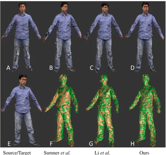
Source/Target Sumneret al. Liet al. Ours
Figure 3.1: Comparison of various algorithms aligning the source surface (E) to the target surface (A). (B)(C)(D) show the deformed source surfaces with three algorithms (Sumner et al., Li et al., and ours) respectively; (F)(G)(H) show deformed source surfaces over target surfaces where the source is in green and the target in orange. Note neither method of Sumner
et al. nor that of Liet al. is able to align the head part correctly, while our method gives exact alignment by using color consistency constraints.
CHAPTER 4: Dynamic Surface Reconstruction
In this chapter, we introduce a 3D capture system that first builds a complete and accurate 3D model for dynamic objects (e.g., human body) by fusing a data sequence captured by mul-tiple commodity depth and color cameras (e.g., Microsoft Kinects), and then tracks the fused model to align it with following captures. One crucial component of our system is the nonrigid alignment which has been introduced in Chapter 3. Our system also extends the volumetric fusing algorithm (Curless and Levoy, 1996; Newcombe et al., 2011) to accommodate noisy 3D data during the scanning stage. We introduce the scanning system in Sec. 4.2, and the tracking system in Sec. 4.3.
4.1 Related work
KinectFusion shows successful scanning of static scenes in real-time in Newcombe et al. (2011) and shows results on processing dynamic objects with piece-wise rigid matching in Izadi et al. (2011). Our work aims at scanning and tracking dynamic objects by employing a non-rigid alignment algorithm.
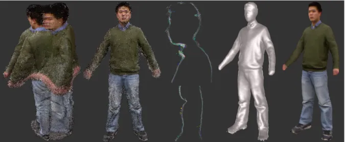
(a) Pre-aligned Point Clouds (b) Post-aligned Point Clouds (c) Cross Section of alignment (d) Fused Scan (e) Fused Scan with Color Figure 4.1: Scanned Dynamic Objects. (a)&(b) show 150 frames of point clouds of one moving person before and after alignment. (c) shows the cross section of the aligned surfaces at the upper body and leg (surfaces are assigned different colors). (d)&(e) show the fused 3D model.
for large deformations and motion of the subjects being scanned and makes no assumption on their shapes.
Our work also relates to research into motion/performance capture of articulated dynamic objects (Gall et al., 2009; Vlasic et al., 2008; Ballan and Cortelazzo, 2008). These works presume a template surface model of the object being tracked is available. They also need a manual skinning procedure, i.e., attach the pre-scanned surface to a skeleton structure or kine-matic tree. De Aguiar et al. (2008) abandoned the skeleton and uses a coarse tetrahedral version of the scan instead, but it still involves manual procedures during initialization. Our system in-stead incorporates a scanning procedure that takes advantage of depth sensors and does not need the manual operations such as skinning or rigging. While the systems above typically need to use a blue-screen to get the object silhouette, our system has no such requirement.
char-Figure 4.2: The Scanning System.
1–
5 the steps in Algorithm 1; (A) the Eight-Kinect System Setup; (B) depth maps; (C) color images; (D) volume visualization of the fused DDF from 8 depth maps; (E) volume visualization of the accumulated DDF at the reference so far; (F) the accumulated reference surface so far; (G) the deformation graph on the surface (F).acter mesh and attach it to the surface. Chen et al. (2012) designed a real-time system that transfers user’s motion to any pre-scanned object. The user’s skeleton is tracked from a Kinect camera and is attached to the embedded deformation graph (Sumner et al., 2007) of the charac-ter, and the character is then deformed accordingly. Instead of only transferring user’s motion, we aim at a tight surface alignment between a user’s pre-scan and the later observation. We also work without explicit requirement to track human skeletons allowing support for arbitrary objects.
4.2 Scanning Dynamic Objects
Algorithm 1:Scanning Pipeline
Set the data from the first frame as the reference;
foreach new framedo
1. fuse depth maps to get the DDF;
2. match the reference surface to the new observation;
3. transform the DDF from target to reference;
4. fuse the transformed DDF into MDDF at reference;
5. generate the reference surface from MDDF, and map colors to the surface;
meters. Four of them cover the upper space, and the other four cover the lower space. Our system setup is shown in Fig. 4.2(a).
We use a similar data fusion pipeline as KinectFusion (Izadi et al., 2011; Newcombe et al., 2011). Initially, the data of the first frame is set as the reference; then we repeatedly estimate the deformation between the reference and newly observed data, and fuse the observed data to the reference. More specifically, we perform following steps for each newly observed frame:
1. Convert depth maps from the Kinects to Directional Distance Functions (DDFs, intro-duced in Chapter 3.4), and fuse them into one DDF Ftrg using the method introduced
later in Section 4.2.2.
2. Sample an Embedded Deformation Graph (ED, introduced in Chapter 3.3) from the ref-erence surface, and estimate its parameters with the nonrigid alignment algorithm intro-duced in Chapter 3 to align the reference surface with the new observation (Ftrg and
color images). The parameters for this forward deformation is computed.
3. Compute the backward deformation (from target to reference) according to the forward deformation, and transform the fused DDF from step 1 to the reference, i.e., Ftrg →
4. FuseFrefinto the Multi-Mode Directional Distance Function (MDDF) at reference.
Un-like DDF, MDDF has multiple distance values and direction vectors at each voxel. A de-tailed introduction of MDDF and fusion of multiple DDFs is presented in Section 4.2.2.
5. Finally, generate the reference surface from the MDDF and texture it by all color images observed so far. To texture the surface, we deform the surface to various frames accord-ing to the estimated forward deformations and project each vertex to the image spaces, the color pixels the vertex falls on are averaged to obtain one 3D color vector.
The scanning procedures are summarized in Algorithm 1, and a graphical illustration is given in Figure 4.2. Note that we always align the fused data to following frames, which helps to deal with the error accumulation problem (Izadi et al., 2011; Newcombe et al., 2011). Also note that we do not directly estimate the backward deformation parameters by deforming the target to the reference. This avoids generating an embedded deformation graph from the noisy surface model at target.
4.2.1 DDF Transformation from Target to Reference
Given the forward deformation parameters{hAj, tji}, we could set the backward
deforma-tion parameters as{hA−j1,−tji} and the graph node position as gj +tj; however it does not
guarantee a backward alignment, since the inverse of the linear interpolation of matrices{Aj}
correspon-Algorithm 2:DDF transformationFtrg → Fref
foreach i-th voxel ofFtrg at locationpi with direction to nearest surface point denoted
asPi and distance value asDido
1. findpi’s nearest point on target surface whose neighboring ED nodes are used for
later deformation;
2. deform its location according to Eq. 3.1: pi →p˜i; 3. deform its directionPiaccording to Eq. 3.2: Pi →Pi˜;
4. record the deformed voxel as a 4-tuplehpi,p˜i,P˜i, Dii; foreach each voxel ofFref at locationqdo
1. find the set of its neighboring deformedFtrgvoxel:
S={hpk,p˜k,P˜k, Dki|kp˜k−qk<};
2. DivideSin to subgroup{Gi}by clustering onp; 3. Find the subgroupGswith smallest averagedD; 4. set the direction and distance value ofFref atq:
Pref =P
k∈Gswk ˜
Pk Dref =P
k∈GswkDk
wherewk =exp(−(q−p˜k)2)
dence intoEcon.
With the backward deformation estimated, one way of deforming the DDF is first gen-erating the underlying triangulated surface from the DDF, then deforming the surface, and eventually re-computing the new DDF from the deformed surface. This method seems plausi-ble, but the DDF field structure is not preserved during transformation due to downgrading the DDF to a surface. We choose to directly apply deformation on DDF. Although the nonrigid transformation is only defined on the surface, each voxel of the DDF could be transformed according to the deformation parameters of its closest point on the surface. Alg. 2 shows our solution of deforming DDFFtrg toFref according to the deformation graph G. Note that we
need to handle the situation when the transformed voxels collide with each other. At each voxel position onFref, we find its nearby transformedFtrg voxels, then group them according
Figure 4.3: Fusing two 2D truncated signed distance fields. (a) shows two curves and their signed distance fields in red and blue respectively. Directly adding two signed distance fields ends up with expanded curves shown in green. (b) shows the signed two distance functions along one line across two curves in red and blue, and the sum of the two in green. (c) shows the above expansion effect is prevent by taking the one with smaller absolute value.
which the direction vector and signed distance value for theFref voxel are interpolated.
4.2.2 Fusion of multiple DDFs
level. Unfortunately, in the case of Fig. 4.3(a), when a big µis chosen to suppress the noise, the zero-crossing of the fused distance field does not align with the surface anymore due to the interference between the distance functions of the front and back surface. This is exactly the case when performing dynamic object scanning via commodity depth cameras, since the noise is evident in the depth maps, due to sensor noise, calibration error and nonrigid alignment, and it can easily go beyond the dimension of thinnest part of the object, such as a palm or wrist.
Fortunately, in many cases, ∇Ddifferentiates which surface a distance value corresponds to. And in our DDF representation, ∇Dcan be easily obtained using Eq. 3.10. When fusing DDFs, at each voxel, we only sum over the distance valueDwith similar∇D, preventing the interference between the distance fields corresponding to different surface parts. This results in a new data structure: Multi-Mode Directional Distance Function (MDDF). Each voxel of a MDDF records a set of averagedD’s, ∇D’s, and the weights on all modes. In our scanning Step 4, a newFref can be easily fused to MDDF. First, the mode with most similar∇Dis found
at each voxel; then its distance value and∇Dis incorporated to that mode and the weights are updated.
4.3 Dynamic Surface Tracking
After fusing a number of DDFs (a few hundreds in our case), the improvement on a scanned model tends to converge. Thus, after a complete model is achieved, we deform the scanned model to the current depth and color observations, i.e., only Steps 1 and 2 in Algorithm 1 are used during this stage—tracking. Note that a fixed Deformation Graph structure is used in Step 2 during tracking.
To track fast moving surfaces, we use a Kalman Filter to predict the translation vectortjfor
each deformation graph node of the next frame , and use its prediction as the initial parameter of the non-rigid alignment problem. The matrices{Aj}are simply initialized using the values
of the last frame.
4.3.1 Tracking Surfaces with Isometric deformations
In many cases, the surface being tracked is roughly under isometric deformations (Bron-stein et al., 2006), i.e., the geodesic distance of any pair of surface points is preserved during deformation. For example, the deformation of the 3D human body model is near isometric, if not strictly isometric. Thus, for these cases, we add a new termElento our energy minimization problem in Eq. 6.3,
Elen(G) =
J X
j=1
X
k∈N(j)
k|gj+tj −gk−tk| − |gj −gk|k
2
2. (4.1)
wheregj andtj are the node location and translation vector of the Deformation Graph
of the edge connecting the neighboring nodes during deformation. Although Elen does not guarantee an exact isometric deformation, in practice it works well to prevent the surface from stretching or shrinking. In our implementation, we use the robust estimation technique (Agar-wal and Mierle, 2013) onElento allow for length changes for some parts (outliers).
4.4 Experimental Results
To test our system, we captured several sequences of people performing various movements using the eight Kinects setup shown in Fig. 4.2(A). Both depth maps and color images from Kinects are used for nonrigid matching, and both have a resolution of640 ×480. Since the depth coming from Kinects deviates from the true depth value (Beck et al., 2013), we correct this depth bias using a linear mapping function for each Kinect separately.
The resolution of the lattice of the volumetric representation (DDF) is set to 1cm in our experiment to reduce the processing time and memory, yet it is still enough to output relatively high quality models. The DDF with higher resolution is necessary to achieve the quality of a high-grade commercial laser scanner. In all of our experiments, µin DDF is set to 4cm; the weights in Eq. 6.3 are set as follows,wrot= 30,wreg = 5.0,wcon = 1.0,wdns pts = 5.0,wclr =
Figure 4.4: Scanning Errors (in cm). The solid lines indicate the mean deviation of the fused surface to the observed surface at each frame on four data sequence. The dashed line shows the standard deviation of the error.
During scanning or tracking, around 150 pairs (per image pair) of matched corner points from the current and previous frame are found via LK optical flow. The points of the previous frame are transformed to the reference via the backward deformation. Note that Edns pts and Eclr only work when the initialization is reasonably close to the optimal solution. Thus, when
the object moves fast and the initial is far off the optimal, Econ plays an important role.
Oth-erwise, it is overwhelmed by Eclr—dense color matches. In our experiment, we ignore Econ
in our tracking state to save us from computing the backward deformation and use the Kalman Filter to predict a reasonable initial value.
4.4.1 Scanning
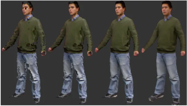
Figure 4.5: Intermediate Scans at frame 1, 5, 15, 30, 50, 80, and 150.
Fig. 4.6 also shows the color on the vertices of the model averaged from all the frames used for fusing (200~300 frames). The sharpness of the color indicates that the frames are well aligned. Be aware that the sparseness of the model vertices (due to the low DDF resolution) leads to some blur from the color interpolation during GPU rasterization. A few intermediate models created during scanning are shown in Fig. 4.5. The noise is gradually filtered out and holes filled up while the geometry details are preserved when accumulating more and more frames.