Statistical inference for the linear model with clustered data

STATISTICAL INFERENCE FOR THE LINEAR MODEL WITH CLUSTERED DATA

Jeffrey J. Harden

A thesis submitted to the faculty of the University of North Carolina at Chapel Hill in partial fulfillment of the requirements for the degree of Master of Arts in the Department of Political Science (American Politics).

Chapel Hill 2009

ABSTRACT

JEFFREY J. HARDEN: Statistical Inference for the Linear Model with Clustered Data (Under the direction of Thomas M. Carsey.)

ACKNOWLEDGMENTS

TABLE OF CONTENTS

LIST OF TABLES . . . v

LIST OF FIGURES . . . vi

Introduction . . . 1

The Problem of Clustering . . . 2

OLS and MR . . . 4

Standard Error Calculation Methods . . . 5

Monte Carlo Simulations . . . 7

Objectives . . . 7

Experimental Model Estimation . . . 9

The Simulation Procedure . . . 10

Results . . . 11

Number of Clusters . . . 11

Sample Size . . . 13

Intra-cluster Correlation . . . 14

Error Term Distribution . . . 16

Discussion . . . 18

An Application: Clustered Data in State Politics Research . . . 19

Original Results . . . 20

Accounting for Clustering . . . 21

MR Replication . . . 23

Conclusions . . . 24

APPENDIX . . . 26

Computational Information . . . 26

Coverage Probability . . . 26

SampleRcode . . . 27

LIST OF TABLES

Table

1 Monte Carlo Simulation Dynamics . . . 9 2 Independent Variables in Hogan (2008, Table 2) . . . 20 3 OLS and MR Models Predicting Challenger Spending as a Percentage of

LIST OF FIGURES

Figure

1 Normal and Student’st(3) Distributions . . . 8 2 Effects of Increasing the Number of Clusters on OLS and MR Standard Error

Methods forN = 1,200, Normalε, andρ≡0.1 . . . 12 3 Effects of Increasing the Sample Size on OLS and MR Standard Error Methods

forβ2 (cluster-level variable), Normalε, andρ≡0.1 . . . 14

4 Effects of Changing ρ ≡ 0.001 on OLS and MR Standard Error Methods with Normalε . . . 16 5 Effects of Changing the Distribution of ε to a t(3) on OLS and MR Standard

Error Methods forβ2(cluster-level variable) with ρ≡0.1 . . . 17

Introduction

Political science research must often account for problems that arise in the data generating process. One such difficulty that is common in several subfields is the possibility of unmodeled correlation between observations within groups, commonly referred to as “clustering” or “mixed-level data.” Comparative scholars, for example, face this issue when studying the effects of country-level variables on individuals. Similarly, within American politics observations might be clustered in Congressional districts, states, or other smaller units. Several studies show that clustering creates a downward bias in the standard errors of Ordinary Least Squares (OLS) regression coefficients, leading to a higher likelihood of committing a Type I error—rejecting the null hypothesis when it is in fact true (e.g., Cornfield 1978; Moulton 1990; Wooldridge 2002, 2003; Arceneaux 2005).

One approach to solving this problem is to adjust the standard errors to account for cluster-ing. In political science, estimating “robust cluster standard errors” (RCSE) for the coefficient estimates has become popular in recent years, likely due to the ease in which the method can be implemented in several statistical software programs. However, despite the mathematical logic that justifies the use of RCSE, it is necessary to assess their effectiveness, along with that of other standard error methods, in an experimental setting. Recent work suggests that the RCSE method may not be as useful as conventional wisdom indicates (Green and Vavreck 2008; Arceneaux and Nickerson n.d.).

The Problem of Clustering

Several disciplines besides political science, including labor economics, education, and various medical fields commonly encounter clustered data (e.g., Donner and Wells 1986; Moulton 1990; Ukoumunne 2002; Wooldridge 2002, 2003; Donner and Klar 2004). Political science is especially subject to the issue in part because a broad question studied in the discipline is how higher-level features of political systems influence the behavior of actors at lower higher-levels. For instance, comparative and international relations research often examines observations grouped in sub-regional, sub-national, or dyadic units (e.g., Posner 2004; Golder 2006; Kasara 2007; Crescenzi 2007; Danilovic and Clare 2007; McDonald 2007; B¨uthe and Milner 2008). Similarly, within the American context researchers commonly encounter observations grouped in smaller units such as states, media markets, counties, cities, or households (Tolbert, McNeal and Smith 2003; Barreto, Segura and Woods 2004; Carson and Crespin 2004; Wolfinger, Highton and Mullin 2005; Arceneaux and Huber 2007; Arceneaux and Nickerson 2009). Importantly, additional scholarship indicates that not accounting for the clustered nature of the data can pose problems for substantive conclusions, even when there is no omitted variable bias (Carsey and Wright 1998; Zorn 2006; Primo, Jacobsmeier and Milyo 2007; Green and Vavreck 2008).

The Design Effect

In an ideal setting, observations for an analysis would be selected and assigned to treatment and control randomly. This would allow the researcher to assume independence among all observations in the study. However, political science almost never enjoys this level of control. In statistical terms, clustering in the data constitutes a violation of the assumption of independent and identically distributed errors (i.i.d.). This violation creates a “design effect” which generates downward bias in the standard errors (Kish 1965; Donner and Klar 2000). Formally, the measure of the degree to which individuals within clusters are similar to each other is calculated as the valueρ. This value is defined by

ρ= s

2 between

s2

between+s2within

(1)

wheres2_betweenis the average variance of the error term across clusters ands2_within is the average variance within clusters (Green and Vavreck 2008). The design effect combinesρwith the average number of individuals within each cluster to yield a measure of the bias to conventional statistical inference methods for a given sample of data. Formally, the design effect is calculated as

where mis equal to the average number of observations within each cluster (Donner and Klar 2004). From this, conventional OLS standard errors will be biased downward by a factor of p

1 +ρ(m−1). For instance, as Green and Vavreck (2008, 143) report, if the design effect is 4, conventional OLS standard errors will be biased downward by a factor of 2 and thus the threshold for statistical significance at the 0.05 level will be ± 3.92 for a two-tailed test hypothesis test rather than±1.96.

Approaches to Dealing with Clustered Data

To this point, most research on clustered data has assumed that the robust cluster technique adequately estimates the magnitude of the design effect by reporting results in which the RCSE are larger than the OLS SE (e.g., Carsey and Wright 1998; Arceneaux 2005; Zorn 2006). A key focus of this study is whether even the larger RCSE are providing an accurate estimate of coefficient variability. If they are not, then it may be more beneficial for researchers to use another estimation strategy to deal with clustered data.1

However, despite the fact that alternatives do exist, dealing with clustering by adjusting the standard errors is still quite common. Within political science, several studies use some form of robust standard error whenever the presence of clustering seems to exist (e.g., Carsey and Jackson 2001; Branton 2004; Buckley and Westerland 2004; Bonneau 2005; Stratmann 2006; Gabel and Scheve 2007; Berry 2008; Gerber, Green and Larimer 2008).2 Based on this increasing popularity, the goal of the present study is to provide a more rigorous evaluation of the standard error choices available.3 Put differently, I assess the extent to which adjusting standard errors is actually accommodating clustered data.

1_{Several methods are available for analyzing clustered data other than the robust standard error adjustment}

procedure examined here. Another involves aggregating the data up to the level of the clustering. This removes the correlation among within-cluster residuals, but it does so at the cost of degrees of freedom and theoretical richness. As a result, it is usually more advantageous for a researcher to keep the unit of analysis at the lowest level, and adjust the model to accommodate the clustered data. This can be done in several ways, including Generalized Least Squares (GLS) (Greene 2002), Generalized Estimating Equation (GEE) models (Zeger and Liang 1986; Zorn 2006), or Hierarchical Linear Models (HLM) (Raudenbush and Bryk 2002; Gelman and Hill 2007). However, it should also be noted that all of these methods have their own limitations (see Steenbergen and Jones 2002; Zorn 2006; Green and Vavreck 2008; Arceneaux and Nickerson n.d.).

2_{Zorn (2006, 332) reports that the number of articles in the three major political science journals containing}

the term “robust standard error” increased from a minimum of one in 1992 to a maximum of 11 (Journal of Politics) in 2002. An informal survey of these journals in the period since 2002 indicates a continuation of this trend.

3_{Not all of the studies cited here use OLS in their analyses. For simplicity, I only consider linear regression in}

OLS and MR

In addition to testing OLS standard errors, I also consider standard error methods for MR, which is methodologically similar to OLS, but more efficient under certain conditions. A typical OLS model fits the data according to the conditional-mean of the dependent variable (Y) at each fixed value of an independent variable (X), orE[Y|X]. Similar logic applies in a MR model, except that the response is fit according to a conditional-median value.

In any linear regression, model residuals are produced as the predicted values subtracted from the actual values, orYi−Yˆi. OLS minimizes the sum of the squared residuals:

minX(Yi−Yˆi)2. (3)

In contrast, MR minimizes the sum of theabsolute deviations—instead of squaring the residu-als, the method simply sums their absolute values. Through one of two methods4_{, this approach}

fits the regression line such that the number of points above the line is equal to the number below the line:

minX|Yi−Yˆi|. (4)

Both OLS and MR yield linear regression coefficients as a solution to a minimization prob-lem.5 _{The least squares method assumes the error term,ε, is normally distributed with mean}

zero and constant variance. MR assumes a Laplace distribution for the errors, which displays heavier tails than the normal. Desmarais and Harden (n.d.) show that a linear model will be es-timated more efficiently by either OLS or MR depending on how close the empirical distribution of the errors is to each of these assumed distributions. OLS is a more efficient method when the error term is closer to a normal and MR is more efficient when it is closer to a Laplace. Exam-ples of heavy-tailed distributions that favor MR include the Cauchy and low-degree of freedom Student’st. In the present study, I examine the consequences of manipulating the error term to favor the efficiency of one method over the other for the performance of the standard errors.

4_{A common approach to solving for MR parameter estimates is to use the Simplex Algorithm (see Koenker}

2005). Alternatively, a Bayesian approach to the problem utilizes Markov chain Monte Carlo (MCMC) with a Laplace-distributed likelihood function (Yu and Moyeed 2001).

5_{Put differently, just as OLS can be characterized as maximum likelihood estimation (MLE) with a}

Standard Error Calculation Methods

OLS

I conduct this analysis by considering three methods for calculating OLS standard errors: the conventional standard errors (OLS SE), RCSE, and bootstrapping (BSE). In a typical linear model such asY =Xβ+ε, the OLS variance-covariance matrix is calculated as

var-cov( ˆβ) = (XTX)−1·XTΦX·(XTX)−1 (5)

whereΦ=εεT. Ifεis homoskedastic and cov(εi, εj) = 0∀i6=j, thenΦ=σ2Iand Equation 5

reduces toσ2_(XT_X)−1_{. OLS SE can then be calculated as the square-roots of the elements on}

the main diagonal of the variance-covariance matrix. Of course, this assumes that the errors are i.i.d., an assumption violated when clustering is present.

To account for this, RCSE constitute a simple adjustment to Equation 5 in which it is assumed that Φ6=σ2_{I. In this case, the elements on the main diagonal of Φare not constrained to the}

same value (i.e., not constrained to σ2_{) and off-diagonal elements from observations within the}

same cluster are not constrained to be zero, as they are in the conventional calculation. Rather, covariances between observations within the same cluster are estimated empirically from the residuals (see Williams 2000; Green and Vavreck 2008, 142).

This is essentially a slight modification to the procedure of the well-known Huber-White robust standard errors, which are designed to correct for heteroskedasticity (Huber 1967; White 1980, see also Long and Ervin 2000). As with RCSE, the Huber-White method estimates the variance-covariance matrix such thatΦ6=σ2_{I. However, while the elements on the main diagonal}

ofΦare not constrained to the same value, the elements of the off-diagonals (covariances) areall

constrained to zero in the Huber-White method, as in the standard calculation of the variance-covariance matrix. By incorporating the possibility of non-zero variance-covariances within clusters, RCSE are designed to be robust to heteroskedasticityand cluster correlation. However, the assumption that observations from different clusters are independent remains (Williams 2000).

MR

Like in OLS, several methods exist for calculating MR standard errors.6 Here I consider three: the conventional asymptotic standard errors (ASE), a kernel density estimate (KSE), and bootstrapping (BSE). The ASE method is roughly analogous to the method for calculating the conventional OLS SE (Hao and Naiman 2007). The MR asymptotic variance-covariance matrix takes the form

p(1−p)

N ·

1

fεp(0)2

·(XTX)−1 (6)

where p= 0.5 in the case of MR, N is the sample size, and fεp(0)2 is the density of the error

term.7 _{Thus, as in OLS, the matrix is calculated as the product of a scalar and (X}T_X)−1_,

but in the MR case the multiplier, p(1_N−p)· 1

fεp(0)2 is an estimate of the asymptotic variance of

the error term evaluated at the sample median (Hao and Naiman 2007, 45). Once the variance-covariance matrix is calculated, standard errors are then constructed in the usual way, as the square-roots of the elements on the main diagonal. The crucial issue with the ASE method is the same as that of the conventional OLS variance-covariance matrix: it assumes the errors are i.i.d. (Koenker 2005; Hao and Naiman 2007). As is the expectation with the OLS SE, this reliance on asymptotics should cause the ASE to be biased downward under clustering in the data.

The other two MR methods I consider are nonparametric and neither are explicitly designed to accommodate cluster- and individual-level variance like the RCSE. However, they also do not explicitly assume i.i.d. errors, which should allow them to be more robust to clustering. The BSE method for MR is identical to the method for OLS described above. Bootstrapping does not impose a distribution on the data and has been shown to accommodate non-i.i.d. data, and thus it may provide better coverage probability than the ASE.

The KSE method, first introduced by Powell (1991), uses a kernel approximation to con-struct standard errors. It estimates the sampling distribution of the MR model by creating a kernel smooth over the model residuals, then calculates the variance-covariance matrix as the variance of the multivariate kernel density function. This method should be more robust to clustering because it estimates standard errors based on the sample data rather than asymptotic assumptions.

6_{Derivations of several methods can be found in Koenker and Bassett (1978), Powell (1991), Koenker (1994),}

and Koenker and Machado (1999). Analyses of these methods include Rogers (1992), Gould (1992), and Koenker and Hallock (2001).

Monte Carlo Simulations

Next I describe a simulation procedure designed to generate a data set with a random cluster component in the error term, estimate the model repeatedly, and assess the differences in the standard errors calculated by each method. The code used to generate the data structure is based on that of Green and Vavreck (2008); an example is provided in the Appendix.

Objectives

In these simulations I assess the extent to which a 95% confidence interval created from each standard error method actually includes the true parameter estimate in 95% of the repeated Monte Carlo simulations. A standard error that is closer to this 95% standard is considered “better” than one that is further away. This process is described in more detail below.

I conduct the experiment under changing data conditions. First, I simulate data with 5, 10, 25, 40, and 50 clusters. The literature on clustering indicates that adding clusters improves standard error accuracy (e.g., Killip, Mahfoud and Pearce 2004; Arceneaux 2005; Green and Vavreck 2008; Arceneaux and Nickerson n.d.). To test this, I hold the number of observations constant, and divide the data into increasingly more clusters—each with its own unique random effect—to assess how standard error estimates behave. This adds to what is often called the “effective sample size.” The maximum cluster value of 50 is chosen as a realistic reflection of the number of clusters (i.e., states or countries in a region) most scholars in political science can expect.

Next, I consider changes to the sample size by conducting the experiment with 200, 800, and 1,200 observations. These values are selected to reflect realistic sample sizes of studies in political science. Note that sample size is closely related toρ. Consider the formula for the design effect (Equation 2); holdingρconstant, the magnitude of the downward bias to OLS SE will increases as the sample size increases, because more observations will be added to the same number of clusters (see Killip, Mahfoud and Pearce 2004).8

Another important parameter to examine dynamically is the value of ρ itself. Donner and Klar (2004) explain that the effects of adjustments to other parameters—such as sample size or number of clusters—are dependent on ρ. If the level of intra-cluster correlation is low, the

8_{This may seem counterintuitive given the common expectation in social science that increasing sample size}

improves precision. Consider theεεT _{matrix from a linear model estimated on clustered data. This matrix}

is filled with a diagonal of ones, (assumed) zeros in off-diagonal elements corresponding to observations from different clusters, andρin off-diagonal elements corresponding to observations within the same cluster. For a constant number of clusters, as observations are added more cells take on the valueρand fewer take on the value zero. Thus, the matrix begins to look less like the assumedΦ=σ2_{I. This should correspond to deteriorating}

improvement to standard error accuracy from adding clusters is relatively modest. However, ifρ

is large, adding more clusters has a bigger effect (Donner and Klar 2004, 420). For this reason, I conduct the experiments at two values of ρ: 0.001, which is common in medical experiments (Donner and Klar 2004), and 0.1, which is the value used in the Green and Vavreck (2008) study. Finally, I consider the implications of violations to the normality assumption by conducting the experiment with a normal error and one drawn from a Student’st distribution with three degrees of freedom. The t distribution with infinite degrees of freedom is equivalent to the normal, but when it has low degrees of freedom, it takes on heavier tails such that a sample will likely contain more outliers than a sample from a normal. Figure 1 provides a visual comparison of the two distributions. The figure plots the theoretical densities of a normal distribution with

µ= 0 andσ= 1 and atdistribution with three degrees of freedom.

−4 −2 0 2 4

0.0

0.1

0.2

0.3

0.4

Density

Normal

t

((

3

))

Fig. 1: Normal and Student’st(3) Distributions

standard error methods should perform better and when the error is drawn from at(3), the MR methods should perform better.9 _{Table 1 summarizes the dynamic aspects of the study.}

Table 1: Monte Carlo Simulation Dynamics

Variable Name Description

Number of Clusters 5, 10, 25, 40, and 50 clusters Sample Size 200, 800, and 1,200 observations

ρ Assumed values: 0.001, 0.1

Distribution ofε Normal andt(3)

Experimental Model Estimation

To assess the effect of these parameters I construct the following experimental model with dependent variableY, independent variablesX1andX2, and an error termε. These variables are

indexed byNindividual observationsi∈(1, . . . , N) andCclusters of observationsc∈(1, . . . , C).

X1 varies at the individual level and X2 is a cluster-level variable. I assess standard error

performance on both variables.

Yic=α+β1X1ic+β2X2c+εic (7)

Following Green and Vavreck (2008), the model is defined such that α = 0, β1 = 0.85, and

β2= 0.5, although these values can be changed without affecting results. In addition, the error

term (ε) is broken into two components: an individual-level disturbance ei and a cluster-level

disturbanceυc such that

εic=ei+υc. (8)

As mentioned above, in half the experimentei andυc are distributed normally and in half they

are distributed according to a t with three degrees of freedom. Additionally, the error term is uncorrelated with the independent variables to avoid creating bias in the coefficient estimates (Gujarati 2003, 71).

The next step is to select a method for evaluating and comparing the standard error methods. This process is not as straightforward as evaluating different methods for calculating coefficient estimates because the smallest standard errors are not necessarily the correct standard errors. Several methods exist in the literature, including calculating “overconfidence” percentages (Beck

9_{This design slightly favors OLS because it is the MLE for a normal distribution. As mentioned above, the}

and Katz 1995), or comparing the standard deviation of the vector of simulated coefficient estimates with the average standard error (Green and Vavreck 2008).

Another method is to calculate a coverage probability (Newcombe 1998; Bradlow, Wainer and Wang 1999; Platt, Hanley and Yang 2000; Ukoumunne 2002). This involves constructing 95% confidence intervals from the standard errors produced by each simulation and calculating the proportion of these confidence intervals that includes the true parameter. The expectation is that this proportion should be 0.95 if the standard error method is “correct.”10 _{A value less}

than 0.95 indicates a downward bias (i.e., toward Type I errors) and a value greater than 0.95 indicates a conservative (Type II error) bias. I use this method because it is common in the statistics literature and because of its simple interpretation, but results are not dependent on this choice. For example, evaluating standard error performance by comparing the mean standard error from the Monte Carlo replications to the standard deviation of the coefficient estimates from the same replications produces the same substantive conclusions. See the Appendix for a more detailed description of the method.

The Simulation Procedure

The Monte Carlo simulation procedure unfolds as follows withN observations andCclusters. At the three different values ofN (200, 800, and 1,200) the procedure is repeated 10,000 times at each value of C (5, 10, 25, 40, 50). This yields a total of 300,000 simulations.11 A single replication of the simulation procedure operates in the following way:

1. A clustered dataset is constructed according to Equations 7 and 8 with N observations andC clusters.12

2. OLS and MR models are fit to the data.

3. From the OLS model, the coefficient estimates, OLS SE, RCSE, and BSE are extracted. From the MR model, the coefficient estimates, ASE, KSE, and BSE are extracted. 4. The process is repeated until 10,000 replications have been performed.

10_{Results remain the same if another standard, such as 0.50, is set as the confidence interval level.}

11_{See the Appendix for computational information on the simulation procedure.}

12_{I use the same technique as Green and Vavreck (2008) to impose a specified value ofρon the data. This}

involves setting the variance of thepopulationfrom which the cluster-level random effect is drawn, which subjects the empirical value, ˆρ, to sampling error. Atρ≡0.001, the average value of ˆρwas 0.003 with a standard deviation of 0.005 and atρ≡0.1, the average value of ˆρwas 0.097 with a standard deviation of 0.025. Although these values are slightly off from their intended targets, the ordering is consistent. In other words, the smaller population value ofρproduces empirical values that are smaller than the larger population value. For more on calculating

At each value of N and C, this process yields 10,000 coefficient estimates for each parameter in the OLS and MR models and 10,000 estimates for each standard error method and each coefficient. After storing this information, the final step is to calculate the coverage probability of each standard error method.

Results

The results of the simulations indicate that each of the various dynamics outlined in Table 1 affect standard error performance. I present the results graphically across the range of clusters in the simulations. In each graph, the number of clusters is plotted on the x-axis and the coverage probability of each standard error method is plotted on the y-axis. A dashed line is drawn at 0.95 to indicate the standard of what a “correct” 95% confidence interval should cover.

Number of Clusters

Previous studies have found that standard errors are generally biased downward when fewer clusters are present, and improve as the number of clusters increases. Figure 2 provides some support for this finding. The graphs plot the coverage probabilities for the OLS and MR standard error estimates forβ1(left panels) andβ2(right panels) withN = 1,200 observations, a normal

error, andρ≡0.1.

Most notably, these results indicate a difference between how the various methods perform on the individual-level variable and the cluster-level variable and a difference between the MR and OLS standard error methods. First, consider the OLS results in the top-left and top-right panels of Figure 2. For β1, the coefficient on the individual-level variable (top-left panel), the

OLS SE and BSE are nearly perfect—both fall on or just around the 0.95 line across the range of clusters. The lines are so close in this and many subsequent graphs that it is difficult to differentiate the BSE line from the OLS SE line. The RCSE, however, are consistently biased downward. This bias is fairly substantial—about 10 percentage points—at 5 clusters, though it decreases to less than 1 percentage point as the number of clusters increases.

In contrast to OLS β1, the results forβ2, the cluster-level OLS variable (Figure 2, top-right

Next, in the MR results, the standard errors estimated for β1 (Figure 2, bottom-left panel)

are all quite close to the 0.95 level and perform equally well across the range of clusters. The ASE and BSE are essentially directly on the line, which makes differentiating the two difficult, while the KSE exhibit a conservative bias; they are too large by about 2 percentage points. Moving to the bottom-right panel of Figure 2, the results forβ2indicate that the MR standard errors behave

similarly to those of the OLS model. Again, the upward curve exists as the number of clusters increases. In this case, the KSE perform the best, though all three exhibit a downward bias, especially at low cluster values. Indeed, with 5 clusters, the KSE method coverage probability is only about 65% and the BSE and ASE methods produce confidence intervals that cover at about 60%. ● ● ● ● ● 0.5 0.6 0.7 0.8 0.9 1.0

Number of Clusters

Coverage Probability ● ● ● ● ● ● ● ● ● ●

OLS: ββ1 (individual−level variable)

0.95

5 10 25 40 50

OLS SE RCSE BSE ● ● ● ● ● 0.5 0.6 0.7 0.8 0.9 1.0

Number of Clusters

Coverage Probability ● ● ● ● ● ● ● ● ● ● 0.95

OLS: ββ2 (cluster−level variable)

5 10 25 40 50

OLS SE RCSE BSE ● ● ● ● ● 0.5 0.6 0.7 0.8 0.9 1.0

Number of Clusters

Coverage Probability

● ● ● ● ●

● ● ● ● ●

0.95

MR: ββ1 (individual−level variable)

5 10 25 40 50

ASE KSE BSE ● ● ● ● ● 0.5 0.6 0.7 0.8 0.9 1.0

Number of Clusters

Coverage Probability ●

● ● ● ● ● ● ● ● ● 0.95

MR: ββ2 (cluster−level variable)

5 10 25 40 50

ASE KSE BSE

Fig. 2: Effects of Increasing the Number of Clusters on OLS and MR Standard Error Methods forN =

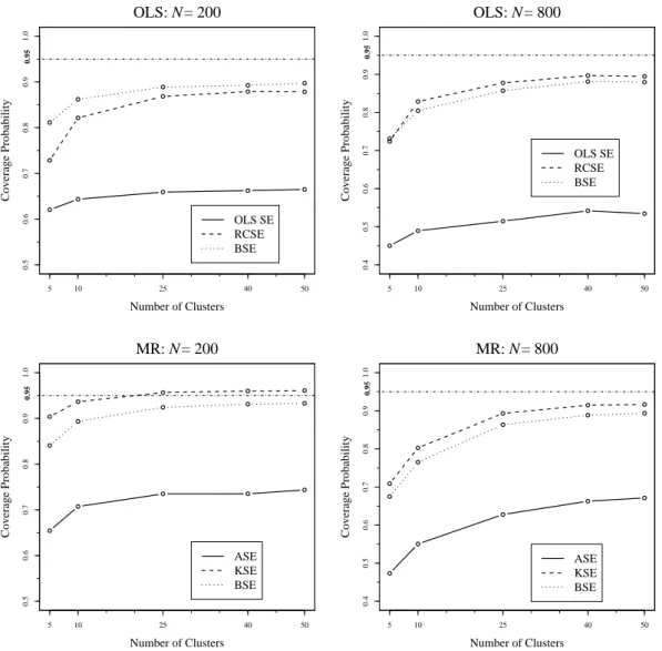
Sample Size

Common intuition of standard errors would suggest that adding observations would improve performance. However, within the context of clustered data, Figure 3 shows that an increase in sample size increases the magnitude of the design effect. The graphs depict the coverage probabilities for the OLS and MR standard error estimates forβ2 under the same conditions as

the right panels of Figure 2, but with the smaller sample sizes ofN = 200 (left panels) andN

= 800 (right panels). Results for β1 are not shown because there is virtually no difference in

performance at different sample sizes for that coefficient.

At the smallest sample size of 200 (Figure 3, top-left panel), all three OLS methods are quite similar; they exhibit the familiar trend upward along the x-axis and all are biased downward (though only by about 1–2% after 25 clusters). In addition, the results indicate that the conven-tional OLS SE are the best method under these conditions. However, moving to the top-right panel of Figure 3 shows that this result changes at a sample size of 800. Again, all three methods show a downward bias, but the RCSE are notably better than the other two methods, even by about 3 percentage points at 50 clusters. Thus, a sample size increase magnifies the downward bias of the OLS SE and BSE but does not alter the performance of the RCSE as much.13

The MR results are slightly different. The simulations performed with a sample size of 200 (Figure 3, bottom-left panel) show the familiar trend upward across the range of clusters. However, a larger separation is evident. No method hits the 0.95 level perfectly. While the BSE are the closest, they are biased slightly downward by about 9 and 4 percentage points, respectively, at 5 and 10 clusters. Additionally, the KSE fall farther away from the 0.95 line, but are generally too large by about 2–3%.

Moving to the sample size of 800 (Figure 3, bottom-right panel), the picture changes slightly. The relative ordering remains the same, with the KSE falling at the highest coverage probabilities across the range of clusters. However, in this case even the KSE exhibit a downward bias at low cluster values, including an extreme of about 73% coverage at 5 clusters. The ASE and BSE are consistently biased downward, though they are only 2–3 percentage points off from the 95% level at 50 clusters.

13_{Comparing the top-right panel of Figure 3 to the top-right panel of Figure 2 indicates that RCSE performance}

● ● ● ● ● 0.5 0.6 0.7 0.8 0.9 1.0

Number of Clusters

Coverage Probability ● ● ● ● ● ● ● ● ● ●

OLS: N = 200

0.95

5 10 25 40 50

OLS SE RCSE BSE ● ● ● ● ● 0.5 0.6 0.7 0.8 0.9 1.0

Number of Clusters

Coverage Probability ● ● ● ● ● ● ● ● ● ●

OLS: N = 800

0.95

5 10 25 40 50

OLS SE RCSE BSE ● ● ● ● ● 0.5 0.6 0.7 0.8 0.9 1.0

Number of Clusters

Coverage Probability ● ● ● ● ● ● ● ● ● ● 0.95

MR: N = 200

5 10 25 40 50

ASE KSE BSE ● ● ● ● ● 0.5 0.6 0.7 0.8 0.9 1.0

Number of Clusters

Coverage Probability ● ● ● ● ● ● ● ● ● ● 0.95

MR: N = 800

5 10 25 40 50

ASE KSE BSE

Fig. 3: Effects of Increasing the Sample Size on OLS and MR Standard Error Methods forβ2

(cluster-level variable), Normalε, andρ≡0.1

Intra-cluster Correlation

Next I consider how changing the level of correlation within clusters influences standard error performance. The left panels of Figure 4 show the results under identical conditions to those in the left panels of Figure 2 (β1,N = 1,200, normal error), but withρ≡0.001 instead of 0.1. This

means that although observations are grouped in clusters, the violation of the i.i.d. assumption is less severe. Similarly, the right panels of Figure 4 shows the simulation results under identical conditions to those in the right panels of Figure 3 (β2, N = 800, normal error), but withρ≡

0.001 instead of 0.1.

near-perfect performances of the OLS SE and BSE remain. However, the OLSβ2 results tell a

much different story. Recall from the top-right panel of Figure 3 that at a sample size of 800 andρ≡0.1, the RCSE perform notably better than the other OLS methods forβ2. In contrast,

whenρ≡0.001 (top-right panel of Figure 4), the RCSE are slightly biased downward at levels of about 19 to 2 percentage points across the range of clusters, while the OLS SE and BSE perform almost precisely at the 0.95 level. In other words, changing the value ofρchanges which standard error method is most accurate when estimated for a cluster-level OLS variable. For a small value ofρ, the conventional OLS SE or bootstrapping are more accurate than the RCSE, but asρincreases, the RCSE perform better.

● ● ● ● ● 0.5 0.6 0.7 0.8 0.9 1.0

Number of Clusters

Coverage Probability

● ●

● ● ●

● ● ● ● ●

OLS: N = 1,200

ββ1 (individual−level variable)

0.95

5 10 25 40 50

OLS SE RCSE BSE ● ● ● ● ● 0.5 0.6 0.7 0.8 0.9 1.0

Number of Clusters

Coverage Probability

● ●

● ● ●

● ● ● ● ●

OLS: N = 800

ββ2 (cluster−level variable)

0.95

5 10 25 40 50

OLS SE RCSE BSE ● ● ● ● ● 0.5 0.6 0.7 0.8 0.9 1.0

Number of Clusters

Coverage Probability

● ● ● ● ●

● ● ● ● ●

0.95

MR: N = 1,200

ββ1 (individual−level variable)

5 10 25 40 50

ASE KSE BSE ● ● ● ● ● 0.5 0.6 0.7 0.8 0.9 1.0

Number of Clusters

Coverage Probability

● ● ● ● ●

● ● ● ● ●

0.95

MR: N = 800

ββ2 (cluster−level variable)

5 10 25 40 50

ASE KSE BSE

Fig. 4: Effects of Changingρ≡0.001 on OLS and MR Standard Error Methods with Normalε

Error Term Distribution

Finally, I consider the implications of changes to the error term distribution on these standard error methods. Recall that only results with a normal error have been presented to this point, and the MR standard error methods have performed comparably well to those of OLS. The results in Figure 5, however, show that violations to the normality assumption can be problematic for OLS. The top and bottom panels, respectively, plot OLS and MRβ2results for a sample size of

200 (left panels) and 800 (right panels) with at(3) error distribution.

even reach the 90% level across the range of clusters.

Two of the three MR methods are less affected by the t(3) error distribution. The bottom panels of Figure 5 show that while the ASE are consistently too small for both sample sizes, the other two methods perform reasonably well, though the increased design effect is quite evident when moving from 200 observations to 800. The KSE appear to be the best choice. They are within 1 percentage point of the 95% standard for most of the range of clusters when the sample size is 200, and are slightly less biased than the RCSE with a sample size of 800, reaching a coverage probability of about 92% with 50 clusters. In comparison, the OLS RCSE only reach 89% coverage under identical conditions.

● ● ● ● ● 0.5 0.6 0.7 0.8 0.9 1.0

Number of Clusters

Coverage Probability ● ● ● ● ● ● ● ● ● ●

OLS: N = 200

0.95

5 10 25 40 50

OLS SE RCSE BSE ● ● ● ● ● 0.4 0.5 0.6 0.7 0.8 0.9 1.0

Number of Clusters

Coverage Probability ● ● ● ● ● ● ● ● ● ●

OLS: N = 800

0.95

5 10 25 40 50

OLS SE RCSE BSE ● ● ● ● ● 0.5 0.6 0.7 0.8 0.9 1.0

Number of Clusters

Coverage Probability ● ● ● ● ● ● ● ● ● ●

MR: N = 200

5 10 25 40 50

0.95 ASE KSE BSE ● ● ● ● ● 0.4 0.5 0.6 0.7 0.8 0.9 1.0

Number of Clusters

Coverage Probability ● ● ● ● ● ● ● ● ● ●

MR: N = 800

5 10 25 40 50

0.95

ASE KSE BSE

Fig. 5: Effects of Changing the Distribution ofεto at(3) on OLS and MR Standard Error Methods for

Discussion

The simulation results show that each of the parameters examined dynamically can influence the performance of these standard error methods. Before addressing these factors, however, it is important to note briefly that the results clearly indicate that adding more clusters to the data is beneficial. Virtually all methods improve or remain constant as the effective sample size is increased. This finding is consistent with previous work on clustering (e.g., Arellano 1987; Moulton 1990; Wooldridge 2002, 2003; Killip, Mahfoud and Pearce 2004; Arceneaux 2005; Green and Vavreck 2008; Arceneaux and Nickerson n.d.).

The results also show a consistent difference in standard error performance depending on the level of the variable for which the standard errors are estimated. For lower-level variables—those that vary at the observational level—the OLS SE outperform the RCSE. In fact, under a normal error, the only instances in which the RCSE actually do improve standard error estimates are for the cluster-level variable. The MR results do not show a clear-cut difference in this regard. The KSE are often the best choice for both levels of variable, though they do tend to be slightly conservative when estimated for lower-level variables.

As previous findings would suggest, an increase in the sample size contributes to increasing bias in the the conventional standard errors for both estimators. Adding more observations magnifies the design effect created by the correlation within clusters. In contrast, the RCSE method performs better than the OLS SE, but still generates biased standard errors when the number of clusters is small. When more clusters are present in the data, the additional residuals provide more information with which to estimate cluster correlation. However, while the RCSE method may be improving inference for the cluster-level variables in a model, it may at the same time be estimating standard errors for individual-level variables that are too small.

Within the MR context, the BSE perform the best at the smallest sample size, but the design effect biases them downward at the larger sample sizes. Though the KSE are slightly too conservative at 200 observations, they display more resistance to the design effect, and actually perform as well or better than the RCSE estimated for the OLS model even when the error term is drawn to favor OLS. For instance, consider the right panels of Figure 3 (N = 800,β2, normal

error,ρ≡0.1). While both the KSE and RCSE are biased downward at the lower cluster values, the KSE fall closer to the 0.95 standard at 25, 40, and 50 clusters (KSE: 0.931, 0.948, 0.955; RCSE: 0.916, 0.934, 0.934).

suggest some changes in this regard as well. While the KSE perform at or near the 0.95 level at

ρ≡0.1, they become slightly too conservative while the BSE perform quite well atρ≡0.001. As expected due to their theoretical reliance on the i.i.d. assumption, the ASE are consistently the most biased MR option in the study. Interested readers who download the replication materials will find that further increasingρleads to all of the methods examined here producing estimates that are increasingly biased downward (although the RCSE display the most resistance to in-creased levels of ρ). Thus, accounting for group-level variation via standard error adjustment may only be feasible at smaller values ofρ.14

Finally, the results indicate that the distribution of the error term is crucial to selecting the appropriate standard error method. Comparing Figures 2–4, with Figure 5 shows a stark contrast between the OLS methods with and without a normal error. While one or more methods perform at close to the 0.95 level under normality, all three OLS methods exhibit a downward bias under thet(3) error term.

In contrast, the MR standard error methods reflect the robustness of the estimation technique, as they are less affected by changes to the distribution ofε. While the ASE are biased downward under both specifications (and more so under thet(3)), the KSE and BSE still perform fairly well. This finding suggests that if a researcher decides to use the standard error adjustment method in dealing with clustered data, one of the first choices made should be that of selecting the correct linear estimator. Desmarais and Harden (n.d.) provide a sample-based test for determining whether OLS or MR is the more efficient linear estimation technique.15

An Application: Clustered Data in State Politics Research

Next I apply the information learned from the Monte Carlo study to existing research in the state politics literature. In “Policy Responsiveness and Incumbent Reelection in State Legisla-tures,” Hogan (2008) examines how the voting behavior of state legislators can influence their chances of reelection. He looks at this process in three specific areas: the decision of challengers to run against incumbents, fundraising success by both challengers and incumbents, and votes received by challengers and incumbents. The data used in the analysis come from approximately

14_{Additional simulation work suggests that HLM provides better standard error estimates than pooled}

regres-sion with RCSE when the value ofρis greater than 0.2.

2,686 incumbents in both the lower and upper houses of 14 states in 1996 and 1998.16

In the current analysis, I focus on replicating the OLS model predicting challenger spending as a percentage of incumbent spending (Hogan 2008, Table 2, 866). The main independent variable,

Partisan Policy Position, is a measure of incumbent divergence from expected district preferences on economic and regulatory policy. This is constructed by regressing legislative voting scores from the National Federation of Independent Business (NFIB) on several district-level measures of demographics, such as income, racial makeup, and education levels. The absolute value of the residuals from this equation are used as a measure of how severely a given incumbent’s voting record diverges from the preferences of the district. A larger residual signifies a legislator whose voting record is strongly divergent from district preferences. Within the context of the challenger spending model, the expectation is that greater divergence will correspond to increased spending by the challengers—an incumbent out of touch with his or her district will draw more significant opposition. The model also includes several control variables, as described in Table 2.

Table 2: Independent Variables in Hogan (2008, Table 2)

Variable Name Description

Partisan Policy Position High values indicate divergence toward party base, away from district median

Political Party 1 = Democrat, 0 = Republican

Major Party Status 1 = Member of majority party,

0 = Member of minority party

Legislative Leadership 2 = Major chamber leader,

1 = Standing committee chair, 0 = Rank-and-file

Party Advantage in District High values indicate support for incumbent’s party

Past Election Vote Percentage Incumbent’s vote share in last general election

District Population (thousands) Number of eligible voters in district divided by number of districts in state

Legislative Professionalism State legislative professionalism (from Squire (2000))

Chamber Competition Percentage of seats held by the minority

party prior to the election

Chamber (upper house) 1 = Upper house, 0 = Lower house

Year 1 = 1998, 0 = 1996

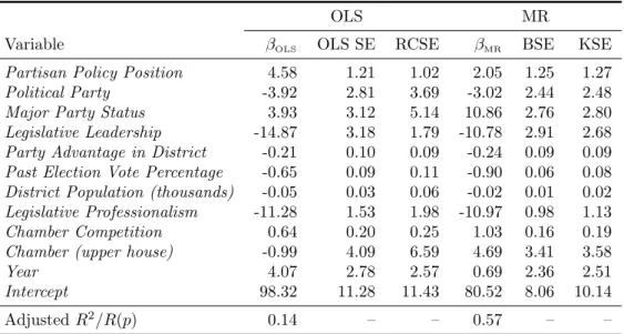
Original Results

In Table 3, columns 1 and 2, I report the original findings presented in Hogan (2008). The first column reports OLS coefficient estimates and the second includes the conventional OLS standard errors. The main result from this model is the positive and significant coefficient on Partisan Policy Position. As Hogan notes, a standard deviation increase in divergence from district

16_{The states represented in the data set are Alaska, California, Florida, Idaho, Illinois, Kentucky, Maine,}

preferences corresponds to an increase of 5% in the challenger/incumbent spending proportion (2008, 867). On average, as an incumbent’s record is increasingly out of step, his or her challenger is able to raise and spend relatively more money.

Table 3: OLS and MR Models Predicting Challenger Spending as a Percentage of Incumbent Spending (Hogan 2008, Table 2)

OLS MR

Variable βOLS OLS SE RCSE βMR BSE KSE

Partisan Policy Position 4.58 1.21 1.02 2.05 1.25 1.27

Political Party -3.92 2.81 3.69 -3.02 2.44 2.48

Major Party Status 3.93 3.12 5.14 10.86 2.76 2.80

Legislative Leadership -14.87 3.18 1.79 -10.78 2.91 2.68

Party Advantage in District -0.21 0.10 0.09 -0.24 0.09 0.09

Past Election Vote Percentage -0.65 0.09 0.11 -0.90 0.06 0.08

District Population (thousands) -0.05 0.03 0.06 -0.02 0.01 0.02

Legislative Professionalism -11.28 1.53 1.98 -10.97 0.98 1.13

Chamber Competition 0.64 0.20 0.25 1.03 0.16 0.19

Chamber (upper house) -0.99 4.09 6.59 4.69 3.41 3.58

Year 4.07 2.78 2.57 0.69 2.36 2.51

Intercept 98.32 11.28 11.43 80.52 8.06 10.14

AdjustedR2_{/R(p) 0.14 – – 0.57 – –}

Note: The dependent variable is challenger spending as a percentage of incumbent

spend-ing. See Hogan (2008, 861–865) for a detailed description of the variables included. R(p)

is a goodness-of-fit measure for MR; see Koenker and Machado (1999) for more details.

The empirical estimate ofρis 0.044. N = 1,816 clustered in 14 state for both models.

Accounting for Clustering

A key issue with this study that is largely unaddressed is the clustered nature of the data.17

If the incumbents in the sample are i.i.d., then inference from the model is straightforward. However, it is theoretically reasonable to suspect that incumbents from the same state may be similar in some way. These incumbents are subject to the same rules and legislative norms while in office, the same campaign finance laws during election season, represent citizens in the same geographic area, handle many of the same issues that are unique within states, and may hold similar cultural or political values. As Arceneaux and Nickerson (n.d.) note, there are many potential similarities that exist within states and are distinct across states that are difficult to model.

Despite the theoretical possibility of within-group similarity, few studies in political science attempt to assess the level of clustering in the data by estimatingρ. This problem can easily be remedied, however, because the process is simple to execute in several different software

packages.18 Using the residuals from the original OLS model reported above, I estimated ˆρ= 0.044 for the model reported above. This value falls within the 0.001–0.05 range that is common in medical trials, but it is difficult to say whether it is typical for a political science study. No systematic study has been undertaken on values ofρwithin the discipline (Green and Vavreck 2008).19

The estimate of 0.044 makes the results comparable to the simulation results presented pre-viously. As a supplement, I performed the simulation procedure under similar conditions to that of the Hogan model (ρ= 0.044, N = 1,816, 14 clusters, normal error). Results indicate that the conventional OLS SE were biased downward for the cluster-level variable, but not the individual-level variable (coverage probabilities of 0.81 and 0.95, respectively) and that the RCSE, though still slightly too small, represented an improvement for the cluster-level variable, but not the individual-level variable (coverage probabilities of 0.88 and 0.92, respectively). From this, my next step was to estimate RCSE for the Hogan model to account for the moderate clustering of incumbents within the same state. They are presented in column 3 of Table 3.

A comparison of the two standard error methods highlights some of the findings from the simulations. For instance, there is a difference in how the RCSE affect inferential leverage based on how each variable varies. Legislative Professionalism, for instance, varies at the state level (i.e., the level of clustering). The RCSE on that coefficient is almost twice the size of the conventional standard error. As is expected from the simulation results, the RCSE provide better coverage for variables that vary at the cluster level. In contrast, the main independent variable,Partisan Policy Position, explains variance only at the individual level, and thus the OLS SE is larger than the RCSE.20 _{The common advice from research on standard errors is to report the largest}

estimate (Green and Vavreck 2008; Arceneaux and Nickerson n.d.). Thus, the OLS SE was the correct choice for the main variable of interest.

18_{InR, ρcan be estimated with the deff() command in the Hmisc package. In STATA, the command is}

loneway. In SPSS, select the “ICC” option from the reliability analysis menu. SAS users must download one of several user-created macros.

19_{I considered two other replications for this study. A model in Golder (2006) produced ˆρ= 0.48 and a model in}

Brown, Jackson and Wright (1999) produced ˆρ= 0.78. Limited simulation work suggests that another technique, such as HLM, may be a better modeling strategy for data clustered at such a high level.

20_{This pattern is broken by some variables. For instance,Political Partyis an individual-level variable, but the}

MR Replication

In addition to the choice of standard error, it is also important to consider which linear estimator is most appropriate. Using the procedure described in Desmarais and Harden (n.d.), I applied the Vuong (1989) and Clarke (2003, 2007) tests to the Hogan model to determine whether OLS or MR provides a more efficient estimate of the parameters. Both tests selected MR as the more efficient estimator.21 _{This suggests that MR is a better method for modeling}

the average effects of the covariates on challenger spending. Further, the Monte Carlo results reported here demonstrate that within the context of clustered data, the BSE and KSE provide the best coverage of MR coefficient variance. As with the OLS model, I supplemented the results by simulating the MR model under conditions similar to the Hogan data. The coverage probabilities for the individual- and cluster-level variables, respectively, were 0.95 and 0.85 for the BSE and 0.97 and 0.88 for the KSE. The fourth, fifth, and sixth columns of Table 3 report MR coefficients and standard errors for the Hogan model.

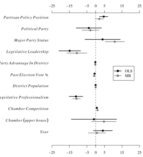
The two MR standard error methods show minor differences. As in the Monte Carlo results, the KSE are generally (though not always) larger than the BSE. Following the recommendation of reporting the largest standard error would mean that the KSE should be reported for all of the variables except Legislative Leadership. Having selected standard errors, next I consider differences between the OLS and MR results for the Hogan model. Figure 6 plots the coefficient estimates (except the intercept) for both models graphically. The circles appear at the point estimate and the lines extending on either side provide a visual depiction of the 95% confidence intervals. These bounds are computed from the largest standard error for each method reported in Table 3.

21_{The Vuong and Clarke tests construct normally- and binomially-distributed test statistics, respectively, from}

−25 −15 −5 0 5 15 25

−25 −15 −5 0 5 15 25

●

●

P arti san P ol i cy P osi ti on

●

●

P ol i ti cal P arty

●

●

M aj or P arty S tatus

●

●

L egi sl ati ve L ead ersh i p

●

●

P arty A d vantage I n D i stri ct

●

●

P ast E l ecti on V ote %

●

●

D i stri ct P opul ati on

●

●

L egi sl ati ve P rof essi onal i sm

●

●

C h amb er C ompeti ti on

●

●

C h amb er ((upper h ouse

))

●

●

Y ear

●

●

OLS MR

Fig. 6: OLS and MR Models of Hogan (2008, Table 2) with Largest Confidence Interval Estimates

The graph indicates that the general substantive story remains unchanged. With one minor exception (Chamber (upper house)), coefficient signs remain the same across the two methods. However, the magnitude of the main independent variable,Partisan Policy Position, weakens in the MR model and the 95% confidence interval (computed from the KSE) crosses the vertical line at zero. Thus, according to the more efficient MR model, the effect ofPartisan Policy Position

is not as strong as originally reported.22

Conclusions

The results from the simulations and replication reported here indicate several points for political scientists to consider when dealing with clustered data. Overall, they show that the

22_{Hogan reports another OLS model with a different dependent variable (2008, 867). It has roughly the same}

standard approach of simply estimating RCSE should not be followed without careful considera-tion of other factors. While the RCSE approach shows some improvement for statistical inference on a mixed-level data model, the method is not an unconditional remedy for clustering.

One common pattern across all of the simulation results is the benefit of adding clusters. Researchers who have control over the data collection process would be better off adding clusters of data rather than additional observations into old clusters. Adding new clusters corresponds to an increase in the “effective sample size” and reduces the bias caused by the design effect, but adding more observations simply increases the magnitude of the design effect. For instance, a state politics researcher could optimize a data collection process by gathering fewer observations from several different states rather than a large number of observations from only a few states.

Next, although no method performs perfectly, these results support the usefulness of Median Regression for political science research. Two of the standard error methods (BSE and KSE) perform fairly well in clustered data, even when the technique’s distributional assumption is violated. In contrast, the OLS methods perform poorly when normality is violated. Thus, this study shows the benefit of estimating the most efficient linear model. The procedure outlined in Desmarais and Harden (n.d.) makes choosing between the two straightforward.

Although political scientists are well aware of clustered data in their own research, almost none of our studies actually measure the degree to which the data are clustered. This study shows that such a measure is crucial for how clustering should be addressed. Estimating RCSE, for instance, really only helps when there is a sufficient level of clustering present. More importantly, the RCSE method actually can have anegative impact on statistical inference if it is used when there is little or no clustering. Thus, generating an empirical estimate ofρshould be a standard model diagnostic if clustering is suspected.

Finally, and perhaps most importantly, the level at which each variable in the model varies should be considered. Both the simulations and replication point out that within OLS, the RCSE only help when the variable is explaining cluster-level variance. In other words, there may be a situation in which the OLS SE perform better than the RCSE even when the data are clustered. For each coefficient, the largest standard error estimate should be reported.

APPENDIX

Computational Information

The Monte Carlo study described here was conducted usingRversion 2.6.1 (R Development Core Team 2008) with the quantreg (Koenker 2008), Design (Harrell 2008a), Hmisc (Harrell 2008b), and mvtnorm (Genz et al. 2008) packages. Two research computing clusters at the University of North Carolina at Chapel Hill were utilized to carry out the simulations. The first, Emerald, is a general purpose 352-processor Beowulf Linux cluster. Simulations on Emerald were performed using the IBM BladeCenter, Dual Intel Xeon nodes with either 2.4GHz/2.5GB RAM, 2.8GHz/2.5GB RAM, or 3.2GHz/4.0GB RAM. The second, Cedar/Cypress is a 136-processor conifers cluster for scientific applications. Jobs were submitted to the login node (Cedar), which holds 8 Intel Itanium2 processors with 1500MHz/8.0GB RAM and completed by the compute node (Cypress), which holds 128 Intel Itanium2 processors with 1600MHz/512GB RAM (RENCI 2008a,b).

Coverage Probability

The coverage probability method for a given standard error and coefficient works as follows. The 10,000 estimates of the coefficient (β) are indexed byj ∈(1,2, . . . ,9,999,10,000). Then a 10,000×3 matrixOis created with each of the 10,000 coefficient estimates in column 2. Columns 1 and 3 are filled with 95% lower and upper confidence bounds calculated from the standard error estimated for β(j). In other words, the standard error is “attached” to its respective coefficient

as a confidence interval, as shown below.

O=                   

β(1)−1.96×SE(1) β(1) β(1)+ 1.96×SE(1)

β(2)−1.96×SE(2) β(2) β(2)+ 1.96×SE(2)

· · ·

· · ·

· · ·

β(9,999)−1.96×SE(9,999) β(9,999) β(9,999)+ 1.96×SE(9,999)

β(10,000)−1.96×SE(10,000) β(10,000) β(10,000)+ 1.96×SE(10,000)

                  

SE* =            

0.0127 0.0171 0.0074 0.0092 0.0231            

O* =            

0.825108 0.85 0.874892 0.786484 0.82 0.853516 0.775496 0.79 0.804504 0.891968 0.91 0.928032 0.834724 0.88 0.925276            

I* =             1 1 0 0 1            

Next, the proportion of ones recorded byI(·) is calculated to produce the coverage probability for that standard error method. In the stylized example, the value 3₅ = 0.6 would be recorded because three of the five simulations produced confidence intervals that covered the true parame-ter. This process is conducted for each standard error method/coefficient combination, providing a measure with which to compare performance under the changing conditions outlined above. The random number generator seed is set to a common value across all simulations for maximum experimental control and reproducibility.

Sample Rcode

1 # "Statistical Inference for the Linear Model with Clustered Data"

2 #

3 # Jeffrey J. Harden

4 # University of North Carolina at Chapel Hill

5 # [email protected]

6 #

7 # last update: January 29, 2009 8 #

9 ###########################################################################

10 # Table of contents:

11 # PART I: Loading packages

12 # PART II: Creating 95% CI coverage counting function

13 # PART III: Monte Carlo simulations 14 #

15 # Requires packages quantreg, mvtnorm, Design, and Hmisc

16 #

17 # This code is based on the STATA code used in:

18 # Green, Donald P. and Lynn Vavreck. 2008. Analysis of Cluster-Randomized Experiments: 19 # A Comparison of Alternative Estimation Techniques." Political Analysis 16(2):138-152.

20 #

21 ###########################################################################

22 # PART I: Loading packages

23 library(quantreg) 24 library(mvtnorm) 25 library(Design) 26 library(Hmisc) 27 # 28 ########################################################################### 29 # PART II: Creating 95% CI coverage counting function (thanks to Bruce Desmarais)

30 comp <- function(bse, p){

31 return(as.numeric(p >= bse[1] - 1.96 * bse[2] & p <= bse[1] + 1.96 * bse[2]))

32 }

33

34 counter <- function(bse, par){

35 return(mean(apply(bse, 1, comp, p = par)))

36 }

37

38 ########################################################################### 39 # PART III: Monte Carlo simulations

40

41 # Control panel

43 n <- 1200 # Sample size 44 nc <- 50 # Number of clusters

45 p <- .1

46 sims <- 10000 # Number of Monte Carlo simulations

47 boot <- 200 # Number of bootstrap replications 48 a <- 0

49 B1 <- 0.85

50 B2 <- 0.5

51 cluster <- rep(1:nc, each = n/nc) # Cluster label

52

53 OLS.B1 <- numeric(sims) # Vectors to store coefficient and SE estimates 54 OLS.B2 <- numeric(sims)

55 OLS.SE1 <- numeric(sims)

56 OLS.SE2 <- numeric(sims)

57 OLS.RCSE1 <- numeric(sims) 58 OLS.RCSE2 <- numeric(sims) 59 OLS.BSE1 <- numeric(sims)

60 OLS.BSE2 <- numeric(sims)

61

62 MR.B1 <- numeric(sims)

63 MR.B2 <- numeric(sims) 64 MR.ASE1 <- numeric(sims)

65 MR.ASE2 <- numeric(sims)

66 MR.KSE1 <- numeric(sims)

67 MR.KSE2 <- numeric(sims)

68 MR.BSE1 <- numeric(sims) 69 MR.BSE2 <- numeric(sims)

70 rho <- numeric(sims)

71

72 for (i in 1:sims){ # Simulate a clustered data set, estimate OLS and MR models

73

74 c.sigma <- matrix(c(4, 0, 0, p), ncol = 2) # Cluster-level random effects

75 c.values <- rmvnorm(n = nc, sigma = c.sigma)

76 randeff1 <- rep(c.values[ , 1], each = n/nc)

77 randeff2 <- rep(c.values[ , 2], each = n/nc)

78

79 i.sigma <- matrix(c(1, 0, 0, (1 - p)), ncol = 2) # Individual-level random effects

80 i.values <- rmvnorm(n = n, sigma = i.sigma)

81 randeff3 <- i.values[ , 1]

82 randeff4 <- i.values[ , 2]

83

84 X1 <- 3 + randeff1 + randeff3 # X1 values unique to individual observations

85 X2 <- randeff1 # X2 values unique to clusters of observations

86 epsilon <- randeff2 + randeff4 # Two components of the error term

87

88 Y <- a + B1*X1 + B2*X2 + epsilon # True model 89

90 fit.ols <- ols(Y ˜ X1 + X2, x = TRUE, y = TRUE) # Model fitting

91 fit.mr <- rq(Y ˜ X1 + X2)

92

93 OLS.B1[i] <- fit.ols$coef[2] 94 OLS.B2[i] <- fit.ols$coef[3]

95 OLS.SE1[i] <- sqrt(fit.ols$var[2, 2])

96 OLS.SE2[i] <- sqrt(fit.ols$var[3, 3])

97 OLS.RCSE1[i] <- sqrt(robcov(fit.ols, cluster)$var[2, 2])

98 OLS.RCSE2[i] <- sqrt(robcov(fit.ols, cluster)$var[3, 3]) 99 OLS.BSE1[i] <- sqrt(bootcov(fit.ols, B = boot)$var[2, 2]) 100 OLS.BSE2[i] <- sqrt(bootcov(fit.ols, B = boot)$var[3, 3])

101

102 MR.B1[i] <- fit.mr$coef[2]

103 MR.B2[i] <- fit.mr$coef[3]

104 MR.ASE1[i] <- sqrt((summary(fit.mr, se = "iid", covariance = TRUE)$cov)[2, 2]) 105 MR.ASE2[i] <- sqrt((summary(fit.mr, se = "iid", covariance = TRUE)$cov)[3, 3])

106 MR.KSE1[i] <- sqrt((summary(fit.mr, se = "ker", covariance = TRUE)$cov)[2, 2])

107 MR.KSE2[i] <- sqrt((summary(fit.mr, se = "ker", covariance = TRUE)$cov)[3, 3])

108 MR.BSE1[i] <- sqrt((summary(fit.mr, se = "boot", R = boot, covariance = TRUE)$cov)[2, 2]) 109 MR.BSE2[i] <- sqrt((summary(fit.mr, se = "boot", R = boot, covariance = TRUE)$cov)[3, 3]) 110

111 rho[i] <- as.numeric(deff(epsilon, cluster)[3])

112 if (rho[i] < 0){

113 rho[i] <- 0 114 }

116

117 OLS.cover1 <- counter(cbind(OLS.B1, OLS.SE1), B1) # Coverage probability

118 OLS.cover2 <- counter(cbind(OLS.B2, OLS.SE2), B2)

119 OLS.rccover1 <- counter(cbind(OLS.B1, OLS.RCSE1), B1)

120 OLS.rccover2 <- counter(cbind(OLS.B2, OLS.RCSE2), B2) 121 OLS.bcover1 <- counter(cbind(OLS.B1, OLS.BSE1), B1) 122 OLS.bcover2 <- counter(cbind(OLS.B2, OLS.BSE2), B2)

123

124 MR.cover1 <- counter(cbind(MR.B1, MR.ASE1), B1)

125 MR.cover2 <- counter(cbind(MR.B2, MR.ASE2), B2) 126 MR.kcover1 <- counter(cbind(MR.B1, MR.KSE1), B1) 127 MR.kcover2 <- counter(cbind(MR.B2, MR.KSE2), B2)

128 MR.bcover1 <- counter(cbind(MR.B1, MR.BSE1), B1)

129 MR.bcover2 <- counter(cbind(MR.B2, MR.BSE2), B2)

130

131 OLS.mean1 <- mean(OLS.B1) # Coefficient means 132 OLS.mean2 <- mean(OLS.B2)

133 MR.mean1 <- mean(MR.B1)

134 MR.mean2 <- mean(MR.B2)

135

136 OLS.meanse1 <- mean(OLS.SE1) # Standard error means 137 OLS.meanse2 <- mean(OLS.SE2)

138 OLS.meanrcse1 <- mean(OLS.RCSE1)

139 OLS.meanrcse2 <- mean(OLS.RCSE2)

140 OLS.meanbse1 <- mean(OLS.BSE1)

141 OLS.meanbse2 <- mean(OLS.BSE2) 142 MR.meanase1 <- mean(MR.ASE1)

143 MR.meanase2 <- mean(MR.ASE2)

144 MR.meankse1 <- mean(MR.KSE1)

145 MR.meankse2 <- mean(MR.KSE2)

146 MR.meanbse1 <- mean(MR.BSE1) 147 MR.meanbse2 <- mean(MR.BSE2)

148

149 OLS.sd1 <- sd(OLS.B1) # Coefficient standard deviations

150 OLS.sd2 <- sd(OLS.B2)

151 MR.sd1 <- sd(MR.B1) 152 MR.sd2 <- sd(MR.B2)

153 avgrho <- mean(rho)

154

155 results <- cbind(OLS.cover1, OLS.cover2, OLS.rccover1, OLS.rccover2, OLS.bcover1,

156 OLS.bcover2, MR.cover1, MR.cover2, MR.kcover1, MR.kcover2, MR.bcover1, MR.bcover2, 157 OLS.mean1, OLS.mean2, MR.mean1, MR.mean2, OLS.meanse1, OLS.meanse2, OLS.meanrcse1,

158 OLS.meanrcse2, OLS.meanbse1, OLS.meanbse2, MR.meanase1, MR.meanase2, MR.meankse1,

159 MR.meankse2, MR.meanbse1, MR.meanbse2, OLS.sd1, OLS.sd2, MR.sd1, MR.sd2, avgrho)

160

REFERENCES

Arceneaux, Kevin. 2005. “Using Cluster-Randomized Field Experiments to Study Voting Be-havior.”Annals of the American Academy of Political and Social Science 601(1):169–179.

Arceneaux, Kevin and David W. Nickerson. 2009. “Who Is Mobilized to Vote? A Re-Analysis of 11 Field Experiments.”American Journal of Political Science53(1):1–16.

Arceneaux, Kevin and David W. Nickerson. n.d. “Modeling Certainty with Clustered Data: A Comparison of Methods.” Unpublished manuscript.

Arceneaux, Kevin and Gregory Huber. 2007. “Identifying the Persuasive Effects of Presidential Advertising.”American Journal of Political Science51(4):957–977.

Arellano, Manuel. 1987. “Computing Robust Standard Errors for Within-Groups Estimators.”

Oxford Bulletin of Economics and Statistics49(4):431–434.

Barreto, Matt A., Gary M. Segura and Nathan D. Woods. 2004. “The Mobilizing Effect of Majority-Minority Districts on Latino Turnout.”American Political Science Review98(1):65– 75.

Bassett, Gilbert and Roger Koenker. 1978. “Asymptotic Theory of Least Absolute Error Re-gression.”Journal of the American Statistical Association73(363):618–622.

Beck, Nathaniel and Jonathan N. Katz. 1995. “What to Do (And Not to Do) With Time-Series Cross-Section Data.”American Political Science Review89(3):634–647.

Berry, Christopher. 2008. “Multilevel Government and the Fiscal Common-Pool.” American Journal of Political Science52(4):802–820.

Bonneau, Chris W. 2005. “What Price Justice(s)? Understanding Campaign Spending in State Supreme Court Elections.”State Politics and Policy Quarterly5(2):107–125.

Bradlow, Eric T., Howard Wainer and Xiaohui Wang. 1999. “A Bayesian Random Effects Model for Testlets.”Psychometrika64(2):153–168.

Branton, Regina P. 2004. “Voting in Initiative Elections: Does the Context of Racial and Ethnic Diversity Matter?” State Politics and Policy Quarterly4(3):294–317.

Brown, Robert D., Robert A. Jackson and Gerald C. Wright. 1999. “Registration, Turnout, and State Party Systems.”Political Research Quarterly52(3):463–479.

B¨uthe, Tim and Helen V. Milner. 2008. “The Politics of Foreign Direct Investment into Develop-ing Countries: IncreasDevelop-ing FDI through International Trade Agreements?” American Journal of Political Science52(4):741–762.

Carsey, Thomas M. and Gerald C. Wright. 1998. “State and National Factors in Gubernatorial and Senatorial Elections.”American Journal of Political Science42(3):994–1002.

Carsey, Thomas M. and Robert A. Jackson. 2001. “Misreport of Vote Choice in U.S. Senate and Gubernatorial Elections.”State Politics and Policy Quarterly1(2):196–209.

Carson, Jamie L. and Michael H. Crespin. 2004. “The Effect of State Redistricting Methods on Electoral Competition in United States House of Representatives Races.” State Politics and Policy Quarterly4(4):455–469.

Clarke, Kevin A. 2003. “Nonparametric Model Discrimination in International Relations.” Jour-nal of Conflict Resolution47(1):72–93.

Clarke, Kevin A. 2007. “A Simple Distribution-Free Test for Nonnested Hypotheses.” Political Analysis15(3):347–363.

Cornfield, Jerome. 1978. “Randomization by Group: A Formal Analysis.”American Journal of Epidemiology108(2):100–102.

Crescenzi, Mark J. C. 2007. “Reputation and Interstate Conflict.”American Journal of Political Science51(2):382–396.

Danilovic, Vesna and Joe Clare. 2007. “The Kantian Liberal Peace (Revisited).” American Journal of Political Science51(2):397–414.

Desmarais, Bruce A. and Jeffrey J. Harden. n.d. “Efficient Estimation of the Linear Model: Choosing Between Conditional-Mean and Conditional-Median Methods.” Unpublished manuscript.

Donner, Allan and George Wells. 1986. “A Comparison of Confidence Interval Methods for the Intraclass Correlation Coefficient.”Biometrics42(2):401–412.

Donner, Allan and Neil Klar. 2000. Design and Analysis of Cluster Randomization Trials in Health Research. New York: Arnold Publishers.

Donner, Allan and Neil Klar. 2004. “Pitfalls of and Controversies in Cluster Randomization Trials.”American Journal of Public Health94(3):416–422.

Efron, Bradley. 1979. “Bootstrap Methods: Another Look at the Jackknife.”Annals of Statistics