The handle http://hdl.handle.net/1887/45135holds various files of this Leiden University dissertation.
Author: Wu, S.
Title: Large scale visual search
Large Scale Visual Search
Proefschrift
ter verkrijging van
de graad van Doctor aan de Universiteit Leiden, op gezag van Rector Magnificus prof.mr. C.J.J.M. Stolker,
volgens besluit van het College voor Promoties
te verdedigen op donderdag 22 december 2016
klokke 16.15 uur
door
Song Wu
geboren te Sichuan, China
Promotor: Prof. Dr. J.N. Kok
Co-promotor: Dr. M.S. Lew
Overige leden: Prof. Dr. A. Plaat
Prof. Dr. W. Kraaij Prof. Dr. T.H.W. Bäck
Prof. Dr. C. Griwodz (University of Oslo)
Prof. Dr. M. Larson (Delft University of Technology)
Copyright c 2016 Song Wu All Rights Reserved
ISBN/AEN 9789463321174
Cover photo: The cover photo shows the flowchart of the proposed deep binary codes used for large scale visual search.
Contents
1 Introduction 1
1.1 Salient Point Methods . . . 2
1.2 Visual Word based Image Search . . . 6
1.3 Convolutional Neural Networks . . . 8
1.4 Thesis Overview . . . 12
2 A Comprehensive Evaluation of Salient Point Methods 17 2.1 Introduction . . . 18
2.2 Background . . . 19
2.3 Overview of Evaluated Salient Point Methods . . . 22
2.3.1 SIFT (detector/descriptor) . . . 23
2.3.2 SURF (detector/descriptor) . . . 25
2.3.3 MSER (detector) . . . 25
2.3.4 HESSIAN-AFFINE (detector) . . . 26
2.3.5 FAST (detector) . . . 26
2.3.6 CenSurE (detector) . . . 27
2.3.7 GFTT (detector) . . . 27
2.3.8 KAZE (detector) . . . 28
2.3.9 BRIEF (descriptor) . . . 28
2.3.10 ORB (detector/descriptor) . . . 29
2.3.11 BRISK (detector/descriptor) . . . 30
2.3.12 FREAK (descriptor) . . . 30
2.3.13 BinBoost (descriptor) . . . 31
2.4 Fully Affine Space Framework . . . 31
2.5 Experimental Setup . . . 34
2.5.1 Datasets . . . 34
2.5.2 Evaluation Criteria . . . 34
2.6 Results and Discussions . . . 35
2.6.1 Detector Evaluation . . . 35
2.6.2 Descriptor Evaluation . . . 38
2.6.3 Affine Invariant Evaluation . . . 41
2.6.3.1 Parameter ofK in K-order NNDR . . . 44
2.6.3.2 Correspondence Matching Using the Framework of Fully Affine Space . . . 45
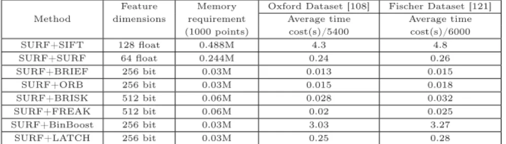
2.6.3.3 Computational Cost and Memory Requirement . 49 2.7 Conclusions . . . 50
3 RIFF: Retina-inspired Invariant Fast Feature Descriptor 51 3.1 Introduction . . . 52
3.2 Discriminate RIFF Local Descriptor . . . 54
3.2.1 Retina Sampling Pattern Review . . . 54
3.2.2 Descriptor Generation . . . 55
3.2.2.1 Orientation Estimation . . . 55
3.2.2.2 Descriptor Generation . . . 56
3.2.2.3 Discriminative Strategy . . . 57
3.3 Visual Word Model based Image Search . . . 58
3.4 Experimental Results . . . 61
3.4.1 Datasets and Evaluation Criteria . . . 62
3.4.2 Evaluation of Image Copy Detection . . . 63
3.4.2.1 Evaluation of Time and Storage . . . 64
3.4.2.2 Evaluation of Search Accuracy . . . 64
3.5 Conclusions . . . 67
4 Deep Binary Codes for Large Scale Image Retrieval 69 4.1 Introduction . . . 70
4.2 Related Work . . . 74
CONTENTS
4.3.1 Generating Deep Binary Codes . . . 75
4.3.2 Spatial Cross-Summing . . . 78
4.3.3 Dynamic Late Fusion . . . 79
4.4 Experiments and Setup . . . 81
4.4.1 Datasets . . . 82
4.4.2 Evaluation of Deep Convolutional Feature Representation . 83 4.4.3 Performance of Deep Binary Codes . . . 84
4.4.4 Comparison with Hashing Learning Approaches . . . 85
4.4.5 Evaluation of the Late Fusion Scheme . . . 87
4.4.6 Performance on Large Scale Image Search . . . 90
4.4.7 Comparison with state-of-the-art . . . 92
4.5 Conclusions . . . 92
5 Comparison of Information Loss Architectures in CNNs 93 5.1 Introduction . . . 94
5.2 Related Work . . . 96
5.3 Convolutional Neural Networks Classification . . . 97
5.4 Integration Architecture Network . . . 98
5.4.1 Concatenate Architecture Network . . . 98
5.4.2 Weighted Integration Architecture Network . . . 99
5.5 Experimental Results . . . 102
5.5.1 Datasets . . . 102
5.5.2 Details of Weighted Integration Architecture . . . 103
5.5.3 Evaluation Results . . . 104
5.6 Conclusions . . . 106
6 Conclusions 107 6.1 Conclusions . . . 107
6.2 Future Work . . . 109
Bibliography 113
English Summary 133
Acknowledgements 137
Chapter 1
Introduction
Content-based image retrieval (CBIR) is one of the important and challenging problems in computer vision research. Frequently used search engines like Google or Yahoo represent a category of text-based information retrieval. However, the search accuracy of text-based information retrieval cannot satisfy the require-ments of users when the text annotations are incomplete or incorrect. More-over, due to the non-scalability of text-based information retrieval to large scale datasets, especially for the ever increasing multimedia data on the web, a high degree of manual effort is required to define the correct text annotations. There-fore, research on content-based information retrieval was proposed to address this issue.
an efficient way.
Benefitting from the advantages of convolutional neural networks (CNNs) [8] trained on sufficiently large and diverse datasets such as ImageNet [9], image representations based on the activations within CNNs have shown significant high performance regarding the state-of-the-art of various computer vision ap-plications. Recent work focuses on investigating effective ways to aggregate the activations within CNNs into compact and distinctive image representations for large scale image search.
Our main research objectives in this thesis are as follows:
• design a robust local descriptor to improve the discrimination of BoW based
image representations.
• provide an effective way for large scale image search by exploring compact
deep binary codes from deep layers within CNNs.
• propose a more powerful CNN architecture to improve the robustness of
the image representation generated from the deep layers in CNNs.
1.1
Salient Point Methods
1.1 Salient Point Methods
Scale space construction: the construction of scale space aims to solve the
challenges in computer vision where the vision information is captured at different scales. The commonly used scale space is the Gaussian smoothed image pyramid which can represent an image at scales and resolutions. The multi-scale representation is achieved by convolving the original image with different Gaussian smooth kernels, and the multi-resolution representation is achieved by down sampling or spatial pooling of the original image.
the additive operator splitting (AOS) scheme [13]. Since the extreme points are detected in discrete scale space, the final scale and location information of these extreme points can be refined by a quadratic fitting operation.
Orientation assignment: assigning each detected salient point an orientation.
The local descriptor of the salient point in images can be represented relative to the calculated orientation and therefore be invariant to image rotation. The orientation assigned by a good measurement can make the generated local descrip-tor more robust to even large image rotation changes. The general orientation measurements can be categorized as: histogram of gradients [14], Haar-wavelet response [12], intensity centroid [15], average gradient of sampling pairs in a pre-designed pattern [16, 17, 18]. The histogram of gradient based orientation is calculated according to the gradient of each pixel within a patch around the
salient point θ(x, y) = arctan(I(x, y)). Then, all θ(x, y) values are counted to
generate a histogram and the maximum bin in the histogram is considered to be the orientation of the salient point. The Haar-wavelet response based orienta-tion is computed according to the responses of Haar-wavelets in both horizontal
and vertical directions in a circle region around the salient point. The domi-nant orientation of the local region is estimated by calculating the sum of all responses within a sliding orientation window covering an angle of 60 degrees, and the largest response is considered as the orientation of the salient point. The intensity centroid approach assumes that the intensity of a salient point is an offset from its center, and it can be used to compute the moments of a patch and further to find its centroid. The orientation is defined as the direction of the vector from the salient point position to the centroid position in the local patch. Some other methods assign orientations to the salient points by averaging the sum of local gradients of the defined pairs in the pre-defined structure.
Local descriptor generation: the local descriptor generation is performed on
1.1 Salient Point Methods
Hand-crafted local descriptors: the hand-crafted schemes mainly explore the
intensity patterns around the detected salient points. The most representative descriptors are the distribution-based local descriptors, which include successful representations such as: histogram of gradients, histogram of gradient orienta-tions, and Haar-wavelet responses distribuorienta-tions, which represent distinctive visual information according to the distributions of pixel intensities in the local patch. Binary local descriptors were proposed with an emphasis on minimizing compu-tational and storage costs. The binary string representations make use of simple pair-wise pixel intensity comparisons. Different binary string local descriptors advocate different pre-defined structures to select the pixel pairs and the gener-ated binary codes can be very efficiently matched with low computational cost using the Hamming metric (bitwise XOR followed by a bit count).
Machine learning based local descriptors: machine learning has been
ap-plied to improve both the efficiency and accuracy of local binary descriptor gen-eration. Hashing is one of the most effective techniques which aims to construct a set of hash functions to map the original input space to compact and similarity-preserving local binary codes. Therefore, similar input spaces could be projected to similar binary codes in the Hamming space. Existing hashing approaches can be divided into two categories: data-independent and data-dependent methods. Data-independent methods randomly generate a projection matrix to map image features into binary representations without training data [19]. The represen-tative methods are locality-sensitive hashing (LSH) [20] as well as its variants [21, 22]. Data-dependent hashing which is also referred to as a hashing learning approach focuses on learning hash functions from a specific training dataset.
[23, 24, 25, 26, 27]. Supervised and semi-supervised hashing approaches take advantage of semantic label information of training data to preserve the ground truth similarity during the construction of binary hash codes. Supervised hashing fully exploits the labeled training data to seek a linear transformation. A loss function is usually defined that penalizes the reconstruction errors between the distances of original data and the distances of corresponding binary data to learn the hash functions [28, 29, 30, 31, 32]. For the case of semi-supervised hashing learning, both unlabeled data and labeled data are utilized to learn the hash functions. For example, the semi-supervised hashing frameworks proposed by Wang et al. [33, 34] minimize the empirical error on the labeled data while max-imizing the variance over labeled and unlabeled data for binary representations. Recently, the deep supervised hashing methods were proposed to learn binary hashing codes. Deep supervised hashing trains a deep hierarchical and nonlinear transformation model and projects the original local descriptors into local binary codes [35, 36, 37, 38].
1.2
Visual Word based Image Search
Content-based image search is still a challenging problem in computer vision. This is mainly due to the existing variations in image appearance, such as the changes of scale, orientation, viewpoint and illumination. In addition, with the increasing amounts of image data on the web, a robust image representation with the approximate nearest neighbor (ANN) search has been widely used for large scale image retrieval. This method is mainly benefiting from the robustness of local descriptors to various geometric transformations and the applicability of different similarity measures.
1.2 Visual Word based Image Search
form a vocabulary of visual words. Therefore, an image is finally represented as a histogram over a set of learned visual words after quantizing each of the local descriptors to the nearest visual word. Early systems [1] used a flat K-means clustering to generate the visual vocabulary, but it was difficult to scale to large vocabularies generation and large scale datasets. The later works [39, 40] show that flat K-means can be scaled to similarly large vocabulary sizes by the use of approximate nearest neighbor methods.
The Fisher Vector (FV) [2] image representation seeks to capture the probability distribution of features. The generative model Gaussian mixture model (GMM) is utilized in FV to estimate a parametric probability distribution over the feature space from a large representative set of local descriptors. The local descriptors extracted from the image dataset are assumed to be sampled independently from this probability distribution. Each local descriptor is represented by the gradient of the probability distribution at that feature with respect to its parameters. Gradients corresponding to all the features with respect to a particular parameter are summed. The final FV representation is the concatenation of the accumulated gradients. They achieve a fixed length vector from a varying set of features that can be used in various discriminative learning activities. Compared with the K-means cluster algorithm, GMM delivers not only the mean information of visual words, but also the shape of their distribution.
Jegou et al. proposed Vector of Locally Aggregated Descriptors (VLAD) [3] which can be viewed as a simplified non-probabilistic version of Fisher Vector. Similar
to the BoW model, a vocabulary withC visual words is first learned via K-means
cluster. Each local descriptor is associated to its nearest visual word in the vo-cabulary. The idea of the VLAD representation is to accumulate the residuals belonging to each of the visual words. This characterizes the distribution of the vectors with respect to the center. A number of variants of VLAD have also been designed to enhance the image representation by considering vocabulary adap-tation and intra-normalization [4], residual normalization and local coordinate systems [5], geometry information [6] and multiple vocabularies [7].
Fisher vector extends the BOW by encoding high-order statistics (first-order and, optionally, second-order), and VLAD is a non-probabilistic equivalent of Fisher Vector. During the past decade, the visual words based image representation has been successfully applied in various computer vision applications.
1.3
Convolutional Neural Networks
Generally, the convolutional neural network (CNN) is a hierarchical architecture [8] which consists of several stacked convolutional layers (optionally followed by a normalization layer and a spatial pooling layer), fully connected layers and a loss layer on top. The convolutional layers generate feature maps by linear convolutional filters followed by nonlinear activation functions (Rectifier, Sigmoid, TanH, etc.). The fully connected layer has full connections to all activations in the feature maps and the resulted one dimensional vector can be fed into the loss layer for loss function optimization.
There are two main stages for training the convolutional neural network: a for-ward stage and a backfor-ward stage. First, the forfor-ward stage is to represent the input image with the current parameters (weights and bias) in each layer. Then the output from the last layer is used to compute the loss function with the ground truth labels. Second, based on the loss cost, the backward stage computes the gradients of each parameter with chain rules. All the parameters are updated based on the gradients, and are prepared for the next forward computation. Af-ter sufficient iAf-terations of the forward and backward stages, the network could be optimized. The convolutional neural network has been applied in diverse com-puter vision applications and demonstrated their significant advantages and high performance.
We will first present an overview of the different types of layers and then briefly review the CNN based computer vision applications.
Convolutional layers: the convolutional layers in the CNN architecture utilizes
k filters (or kernels) to convolve the input image to generate k feature maps.
1.3 Convolutional Neural Networks
parameter sharing mechanism is used in convolutional layers such that the number of parameters could be significantly reduced. Second, local connectivity learns correlations among neighboring pixels. Third, it is invariant to the location of the object. Due to these benefits introduced by the convolution operation, some well-known research papers also use it as a replacement for the fully connected layers to accelerate the learning process [42, 43].
Pooling layers: a pooling layer is an optional layer following a convolutional
layer which sub-samples its input. Average pooling and max pooling are the most commonly used pooling operations. The reason to use a pooling operation in the convolutional neural network is that: first, it can reduce the dimensions of the output and the number of parameters of the network, while keeping the most salient information. Second, a pooling operation also provides basic invariance to translating (shifting) and rotation. For max pooling and average pooling, Boureau et al. [44] provided a detailed theoretical analysis of their performances. Scherer et al. [45] further conducted a comparison between the two pooling operations and found that max-pooling can lead to faster convergence, selection
of superior invariant features and improve generalization.
Fully-connected layers: after several convolutional and max pooling layers,
Recently, deep learning, especially for the CNNs, produced state-of-the-art per-formance on various computer vision applications, such as image classification, image search, object detection, semantic image segmentation, human pose esti-mation, etc.
Image classification: Krizhevsky et al. [48] set a milestone for large-scale
im-age classification when training a large CNN on the Imim-ageNet dataset [9], thus proving that CNN could perform well on natural image classification. OverFeat [49] proposed a multi-scale and sliding window framework, which could find the optimal scale of the image and fulfill different tasks simultaneously, e.g., image classification, object detection and localization. Because the existing CNNs re-quire fixed-size image data as input, the SPP-Net [50] model eliminated this restriction via a spatial pyramid pooling strategy in the CNNs and improved the classification accuracy of a variety of CNN architectures despite their different designs. The later proposed VGGNet [51] and GoogleNet [42] significantly im-proved the performance of image classification by increasing the width and depth of the network architectures.
Object detection: a general scheme for high performance object detection
sys-tems is to generate a large number of candidate object region proposals and classify them using their high performance CNN features. The most representa-tive approach is the regions with CNN features (RCNNs) [46]. It utilizes selecrepresenta-tive search [52] to generate object region proposals, and extracts the CNN features for each candidate region. The features are then fed into a SVM classifier to decide whether the related candidate windows contain the object or not. RCNNs improved the benchmark of object detection by a large margin, and became the base model for many other promising algorithms [53, 54, 55]. Also, the original RCNNs were computationally expensive, the recent works [50, 56] employed the strategy of sharing convolutions across the region proposals to reduce the com-putation cost. The latest frameworks of Fast RCNNs [56] and Faster RCNNs [57] achieve near real-time rates using very deep networks.
Image retrieval: The success of AlexNet [48] suggests that CNNs can be used
1.3 Convolutional Neural Networks
for image classification. Motivated by this, many recent studies make use of the activations of the top fully connected layers in CNNs for image retrieval [58, 59, 60, 61, 62, 63]. Recent researches also suggested to explore the features from the deep convolutional layers in CNNs. These features have very useful properties: first, they can be efficiently extracted from an image of any size and aspect ratio. Second, features from the convolutional layers have a natural interpretation as descriptors of local image regions corresponding to receptive fields of the particular features. Finally, simple pooling operations can aggregate feature maps from deep convolutional layers into low dimensional and highly distinctive features [58, 60, 63, 64, 65]. The CNNs based image representations have demonstrated their competitive and even better results compared with the traditional visual words methods, such as BoW, VLAD and Fisher Vector.
Semantic image segmentation: semantic image segmentation can be referred
to as a problem of pixel-level classification or labeling. Recently, the CNNs and probabilistic graphical models were utilized to address this task and yielded promising progress [66, 67, 68, 69, 70]. The CNN based semantic image seg-mentation methods usually convert an existing CNN architecture constructed for classification to a fully convolutional network (FCN). This is mainly because the FCN architecture accepts a whole image as an input and performs fast and ac-curate inference. Long et al. [68] replaced the last fully connected layers of a CNN by convolutional layers, and obtained a coarse label map from the network by classifying every local region in the image, then performed a simple deconvo-lution, which is implemented as a bilinear interpolation, for pixel-level labeling. DeepLab [69] proposed a similar FCN based model which obtained denser score maps within the FCN framework to predict pixel-wise labels and refined the label map using the fully connected conditional random field (CRF). Instead of using CRF as a post-processing step, Lin et al. [70] jointly trained the FCN and CRFs by efficient piece wise training.
Human pose estimation: estimating the human pose by locating human body
formulated as a CNN-based regression problem towards human body joints. The representative projects [71, 72] proposed to use a cascade of CNN-based regres-sors to reason the positions of body joints or facial landmarks. The cascade of CNNs can be viewed as a kind of holistic process which takes the full image as
the input and output the ultimate position of body joints or facial landmarks in the image without using any explicit graphical model or part detectors. The part-based processing methods propose to detect the human body parts indi-vidually, followed with a graphical model to incorporate the spatial information.
Rather than training the network using the whole image as input, Chen et al. [73] utilized the local part patches to train a CNN, in order to learn conditional probabilities of the part presence and spatial relationships. By incorporating with graphical models, the algorithm gained promising performance. Tompson et al.
[74] designed multi-resolution ConvNet architectures to perform heat-map like-lihood regression for each body part, followed with an implicit graphical model to further promote joint consistency. The model was further extended and im-proved [75], which argues that the pooling layers in the CNN would limit spatial
localization accuracy and try to recover the precision loss caused by the pooling process. Additionally, Fan et al. [76] proposed a dual-source convolutional neu-tral network (DS-CNN) to integrate the holistic and partial view in a two branche CNN architecture. It takes part-patches and body-patches as inputs to combine
both local and contextual information for more accurate pose estimation.
1.4
Thesis Overview
This thesis is based on first-authored conference papers that have been published or journal papers are currently under review. The research has been carried out during the four-year period of the PhD research. The focus of this thesis has been on developing and analyzing techniques to improve the state-of-the-art of
large scale image search.
1.4 Thesis Overview
A survey is presented that evaluates the performance of a wide set of salient point detectors and descriptors. First, the survey compares diverse salient point algorithms with regard to the repeatability of salient point detectors, recall and precision of salient point descriptors. Then, it integrates the salient point meth-ods with the framework of fully affine space and evaluates the performance under major viewpoint transformations. The presented comparative experimental re-sults can benefit researchers in choosing an appropriate detector and descriptor for different computer vision applications. An early version of this work was presented at:
• 21st ACM international conference on Multimedia (MM 2013), in Barcelona,
Spain.
Chapter 3: RIFF: Retina-inspired Invariant Fast Feature Descriptor
We first propose the Retina-inspired Invariant Fast Feature, RIFF, which was de-signed for invariance to scale, rotation, and affine image deformations. The RIFF descriptor is based on pair-wise comparisons over a sampling pattern loosely based on the human retina and introduces a method for improving accuracy by maxi-mizing the discriminatory power of the point set. A performance evaluation with regard to Bag-of-Words based image retrieval on several well-known benchmark datasets demonstrates that the RIFF local descriptor has competitive perfor-mance to the state-of-the-art local descriptors. Additionally, a popular approach from the literature is to use visual words (or Bag-of-Words) constructed from real valued descriptors (SIFT and SURF). To accommodate large scale data sets, we used the approximate nearest neighbor (ANN) based cluster approach to both real valued local descriptors and binary string local descriptors (BRIEF, ORB, BRISK and FREAK) and the results on the test datasets reveal that some of the recent binary string approaches outperformed notable descriptors such as SIFT and SURF. This approach has been presented at the following conferences:
• 22nd ACM international conference on Multimedia (MM 2014), in Orlando,
FL, USA.
• 4th ACM International Conference on Multimedia Retrieval (ICMR 2014),
Chapter 4: Deep Binary Codes for Large Scale Image Retrieval
We present a novel and effective method to create compact binary codes (deep binary codes) based on deep convolutional features for image retrieval. Deep binary codes are generated by comparing the response from each feature map and the average response across all the feature maps on the deep convolutional layer. Additionally, a spatial cross-summing strategy is proposed to directly generate bit-scalable binary codes. As the deep binary codes on different deep layers can
be obtained by passing the image through the CNN and each of them makes a different contribution to the search accuracy, we then present a dynamic,
on-the-fly late fusion approach where the top N high quality search scores from deep
binary codes are automatically determined online and fused to further enhance the retrieval precision. Two strengths of the proposed methods are that the generation of deep binary codes is based on a generic model which does not require additional training for new domain areas, and the dynamic late fusion scheme is query adaptive. Extensive experimental results on well known benchmarks show that the deep binary codes are competitive to state-of-the-art approaches in terms of the performance on large scale image retrieval. Moreover, the search accuracy is shown to be enhanced substantially by the dynamic late fusion scheme. The
paper has been submitted to:
• Journal of Neurocomputing
Chapter 5: Comparison of Information Loss Architectures in CNNs
1.4 Thesis Overview
as an improved performance of the proposed WIAN. The basis for this chapter is formed by the publication in the conference proceeding:
• 17th Pacific-Rim Conference on Multimedia (PCM, 2016) in Xi’an China.
These are the publications which were related to the contents of this thesis:
• Wu S., and Lew M.S., “Evaluation of salient point methods.” Proceedings
of the 21st ACM International Conference on Multimedia. ACM, 2013.
• Wu S., and Lew M.S., “Salient features for visual word based image copy
de-tection.” Proceedings of International Conference on Multimedia Retrieval. ACM, 2014.
• Wu S., and Lew M.S., “RIFF: Retina-inspired Invariant Fast Feature
De-scriptor.” Proceedings of the 22nd ACM International Conference on Mul-timedia. ACM, 2014.
• Wu S., and Lew M.S., “Comparison of Information Loss Architectures in
CNNs.” Proceedings Pacific RIM Conference on Multimedia, 2016.
• Wu S., and Lew M.S., “Image Correspondences Matching Using Multiple
Features Fusion.” Proceedings of European Conference on Computer Vision Workshop, 2016.
• Wu S., Oerlemans A, Bakker E.M., and Lew M.S., “Deep Binary Codes for
Large Scale Image Retrieval.” Journal of Neurocomputing (submitted).
• Wu S., Oerlemans A, Bakker E.M., and Lew M.S., “A Comprehensive
Evaluation of Salient Point Methods.” Journal of Computer Vision and Image Understanding (submitted).
• Guo Y., Liu Y., Oerlemans A., Lao S.,Wu S., and Lew M.S. “Deep learning
for visual understanding: A review.” Journal of Neurocomputing, vol 187, 2016.
• Zhang Q., Zaaijer S., Wu S., and Lew M.S. “3D Image Browsing: The
• Guo Y., Bai L, Lao S.,Wu S., and Lew M.S. “ A Comparison between Arti-ficial Neural Network and Cascade-Correlation Neural Network in Concept Classification.” Proceedings Pacific RIM Conference on Multimedia, 2014.
• Liu Y., Guo Y., Wu S., and Lew M.S. (2015), “DeepIndex for Accurate
Chapter 2
A Comprehensive Evaluation of
Salient Point Methods
2.1
Introduction
Salient point methods which can describe meaningful, stable, and representative local features in an image have become prevalent in diverse areas in computer vision, such as object and scene recognition [77, 78], 3D object reconstruction [79], visual tracking [80, 81] and multimedia information retrieval [3, 18, 82, 83, 84, 85, 86, 87, 88]. Most of the salient point algorithms contain two parts: a detector and a descriptor. The detector locates a set of distinctive points which can be invariant to various transformations (e.g., scaling, translation, viewpoint changes), and the descriptor encodes the important information from the local patch centered on the salient point into a feature vector, which makes it possible to reliably match correspondences across different transformations of the same object or the same scene.
Typically, object recognition, 3D reconstruction and visual tracking mainly rely on the correctly matched correspondences between two compared images. These applications start by extracting local descriptors from each image and insert the obtained local descriptors into an index space for efficient correspondence match-ing. The RANSAC algorithm [89] is further adopted to eliminate outlier matches and to estimate the homography between the compared images. Therefore, a salient point detector with high repeatability and a local descriptor with discrim-inatory power is required for these applications.
2.2 Background
complexity salient point algorithms with the framework of fully affine space and evaluate their performance under the extreme viewpoint changes.
This chapter is an extension of our previous projects [87, 88] which provide a comparison guide of recently proposed salient point detectors and descriptors. The main contributions of this chapter are summarized as follows:
First, the repeatability performance and the computational cost of each salient point detector are presented.
Second, the efficiency and accuracy of both the real valued descriptors and binary string descriptors in terms of recall and precision on two benchmark datasets are evaluated.
Third, we calculate the accuracy and time complexity of each salient point method in the framework of fully affine space such that researchers could make a trade-off between precision and efficiency under extreme viewpoint changes.
2.2
Background
contiguous pixels in a circle are all brighter or all darker than the intensity of the centre point.
Since conventional corner point detectors are only invariant to scale, translation, and noise, affine covariant region detectors were developed to reduce the influence of viewpoint changes. The Harris-Affine detector and the Hessian-Affine detector [97] find the initial candidate points by using the Harris-Laplacian corner detector and Hessian-Laplacian corner detector, respectively, and then fit an elliptical region to each point via the second moment matrix of the intensity gradient. MSER [98] computes the connected binary regions through a large set of multiple thresholds, and the selected regions are those that maintain unchanged shapes over these thresholds. As edges are typically rather stable structures that can be detected over a range of image changes, EBR [99] starts by detecting corner points in an image and identifies the affine covariant region of each point by exploiting the edge information present nearby. IBR [100] detects intensity extrema at multiple scales and captures the intensity pattern along rays emanating from each extremum to define a region of arbitrary shape. The region of IBR is delineated by the image points defined over these rays where the intensity suddenly increases or decreases, and then uses an ellipse to fit the region. However, the operation of elliptical region fitting in the affine covariant detector could result in partial information loss.
2.2 Background
unstable points can be discarded. Root-SIFT [104] adds a square root operation to the normalized SIFT features and uses the Hellinger kernel to increase the matching accuracy. DSP-SIFT [105] generates the descriptor through pooling the gradient histogram across different domain sizes of each salient point into a feature and it even outperforms the high level convolutional neural network feature [48]. Affine-SIFT (ASIFT) [90] is proposed with the aim to be perspective invariant and it does this by simulating images under various views to cover the whole affine space and extracting SIFT descriptors in all these simulated images for matching. Different from these variants of SIFT, other approaches target on improving the efficiency of scale space establishment or accuracy of salient points localization. For example, the SURF detector makes use of a box-filter and the integral image to speed up the scale space building. The ORB and BRISK detectors use a Gaussian image pyramid to efficiently establish the scale space. As the construction of scale space by linear multi-scale Gaussian pyramids easily results in the blurring and the loss of boundary details, KAZE [106] combines a nonlinear scale space with additive operator splitting (AOS) and special conductance diffusion to reduce noise while retaining the object boundary structure. The advantage of the nonlinear scale space in KAZE is that it could provide more accurate positions for salient points.
sam-pling of BRIEF. BRISK and FREAK generate the binary string descriptors by comparing pair-wise intensities over a pre-defined pattern, a concentric ring-based sampling pattern and a retina sampling pattern, respectively. In contrast to those hand-crafted patterns, learning based approaches are proposed with the goal of closing the performance gap with real valued representations while maintaining the benefits of binary representations. BinBoost learns a set of hash functions us-ing boostus-ing and projects the image patch into a binary representation. LATCH proposes to learn patch triplet arrangements in the image and compares the in-tensity of triplet patches rather than the inin-tensity of pixel-pairs to generate the binary codes.
Several related reviews present the performance evaluation of various salient point methods. Schmid et al. [107] uses the measure of “repeatability rate” and “infor-mation content” to evaluate the performance of different salient point detectors. Mikolajczyk et al. [108] made a performance evaluation of local descriptors by measuring the accuracy of matching and recognition. Accuracy and computa-tional efficiency trade-offs [109] have been studied where different indexing struc-tures were employed (such as approximate KD-trees). Heinly et al. [110] and Figat et al. [111] investigate the recall and precision of recent binary string rep-resentations under different image deformations. Gauglitz et al. [81] presents a comparison of different salient point methods on video object tracking. Moreels and Perona [112] made a performance evaluation of both feature detectors and descriptors on 3D object matching. Mukherjee et al. [113] made a performance evaluation for each combination of recent detectors and descriptors on object matching. To our knowledge, our review is the first one that evaluates the view-point invariance of each salient view-point approach in the fully affine space.
2.3
Overview of Evaluated Salient Point
Meth-ods
per-2.3 Overview of Evaluated Salient Point Methods
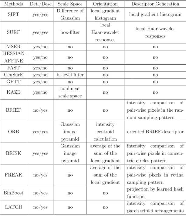
form the image representation. Recent salient point methods consist of four main procedures: the first step is to establish the scale space and find the extrema across all scales to achieve scale invariance. The second step is to determine the locations of the extrema and to define a local region for each according to the scale information. Then, each defined region is normalized and assigned a do-main orientation to be rotation invariant. Finally, the region content is rotated based on the calculated orientation, after which, the discriminative information in the rotated region is encoded into a local descriptor. The existing schemes of local descriptor generation can be categorized into hand-crafted schemes and au-tomatically learned schemes. The recent literature focuses more on the automatic learning of local descriptors. The learning based schemes usually optimize an ob-jective function to generate robust and distinctive local descriptors. In particular, the most common objective functions are designed to minimize the distance be-tween the descriptors from the same 3D coordinate (scale and location) or same class label extracted under varying imaging conditions and different viewpoints, meanwhile, maximizing that distance between patches from different 3D coordi-nates or different class labels. Table 2.1 gives an overview of all the evaluated salient points approaches in the experiments section.
2.3.1
SIFT (detector/descriptor)
Table 2.1: Overview of the evaluated salient point approaches in this chapter by Detector (Det.), Descriptor (Desc.), Scale Space, Orientation, and Descriptor Generation.
Methods Det./Desc. Scale Space Orientation Descriptor Generation
SIFT yes/yes Difference of
Gaussian
local gradient
histogram local gradient histogram
SURF yes/yes box-filter
local Haar-wavelet
responses
local Haar-wavelet responses
MSER yes/no no no no
HESSIAN-AFFINE yes/no no no no
FAST yes/no no no no
CenSurE yes/no bi-level filter no no
GFTT yes/no no no no
KAZE yes/no nonlinear
scale space no no
BRIEF no/yes no no
intensity comparison of
pair-wise pixels in the ran-dom sampling pattern
ORB yes/yes Gaussian image pyramid intensity centroid calculation
oriented BRIEF descriptor
BRISK yes/yes
Gaussian image pyramid
average of the sum of the local gradient
intensity comparison of
pair-wise pixels in concen-tric circles pattern
FREAK no/yes no
average of the sum of the local gradient
intensity comparison of
pair-wise pixels in retina sampling pattern
BinBoost no/yes no no projection by learned hash
function
LATCH no/yes no no intensity comparison of
patch triplet arrangements
potentially sensitive to edge responses. To be invariant to rotation, an orientation
orien-2.3 Overview of Evaluated Salient Point Methods
tation histogram within a region around the point. In addition, it accumulates
the orientations of a 16×16 neighborhood of sample points around the salient
point location into orientation histograms by summarizing the contents over4×4
sub-regions. A 128-dimensional descriptor vector is finally generated to represent each point.
2.3.2
SURF (detector/descriptor)
SURF is an efficient and robust scale and rotation-invariant method proposed by Bay et al. [12] with the aim for fast salient point location and descriptor generation. SURF is based on a Hessian matrix, where the components of the Hessian matrix are generated by convolution of the Gaussian second-order deriva-tive with the image pixels. Box-filters together with integral images are exploited to approximate the Hessian matrix which is used to measure the salient points. The Gaussian scale space of SURF is established computationally efficiently by up-scaling the size of the box-filter. The extrema of the determinant of the Hes-sian matrix are selected as salient points and the scale and location are updated through an interpolating process. Each of the obtained salient points is assigned an orientation which is estimated by summing the horizontal and vertical Haar-wavelet responses within a sliding orientation window covering an angle of 60 degrees. For the SURF descriptor generation, first the square region centered
on and oriented along the salient point is divided into a number of 4×4
sub-square regions. Then, it calculates the value and absolute value of Haar-wavelet responses along horizontal and vertical directions within each sub-region. Finally
the total 64-dimensional (4×4×4) descriptor can be generated efficiently by
making use of the integral image.
2.3.3
MSER (detector)
that maintain unchanged shapes over a range of thresholds. During the affine invariant regions detection, the area of each connected component is stored as a function of intensity and the “maximally stable” ones are selected as candidates by analyzing the changes of function values for each potential region. The final maximally stable extremal regions are the ones that maintain an unchanged or similar function value over a large range of multiple thresholds. The shape of each obtained region is further estimated by elliptical regions by computing the eigenvectors of their second-moment matrix. Then the local neighborhoods are normalized into circular regions to achieve affine invariance.
2.3.4
HESSIAN-AFFINE (detector)
The Hessian-Affine region detector proposed by Matas et al. [97] is based on the Hessian matrix. A related variant of the Hessian-Affine detector is the Harris-Affine detector which employs the Harris detector to find the salient points. Since the second derivatives in the Hessian matrix offer strong responses on blobs and ridges, the extrema of the determinant of the Hessian matrix are searched by
applying non-maximum suppression using a3×3window over the entire image.
To deal with the scale invariance, given an extremum location, a scale-dependent signature function is defined on its local neighborhood and the corresponding scale can be determined by searching for scale-space extrema of the signature function. The estimation of the affine shape is applied to each extremum and an elliptical region is fit around each point using the second moment matrix of the intensity gradient. Finally, the affine region is normalized into a circular region. In this chapter, the improved Hessian-Affine detector [114] is used, which proposes the gravity vector assumption to fix rotation uncertainty.
2.3.5
FAST (detector)
2.3 Overview of Evaluated Salient Point Methods
pixels) of sixteen pixels around the candidate point. If there exists a set of twelve contiguous pixels in the circle which are all brighter or all darker than the intensity of the candidate point pixel value plus a threshold, the point will be classified as a corner point. However, this scheme has a limitation for sampling less than twelve pixels and the efficiency of the corner detector depends on the distribution of corner appearances. To overcome the above weaknesses, a machine learning approach is employed on training sets to establish a decision tree for fast and accurate corner detection. Moreover, the issue of multiple features being detected adjacent to one another, can be solved by applying non-maximum suppression on the detected candidate corner points.
2.3.6
CenSurE (detector)
The scale invariant center-surround salient point detector (CenSurE) is proposed by Agrawal et al. [115]. CenSurE determines the salient points by exploiting the extrema of the Hessian-Laplacian matrix across all scales and locations. In-spired by SIFT which uses the Difference of Gaussian function to approximate the Laplacian of Gaussian function, CenSurE employs a simplified center-surround filter called bi-level filter to approximate the Laplacian of Gaussian for fast com-putation. The CenSurE detector computes the response of the bi-level filter at all locations and all scales, and detects the extrema in a local neighborhood (based on the non-maximum suppression method, which is the same as SIFT and SURF). For each obtained extremum, the accurate location of the potential points can be determined directly, since the responses are calculated on the original image. Furthermore, through computing the Harris measure for the potential points, those points with weak corner responses will be eliminated.
2.3.7
GFTT (detector)
under affine image transformations. According to the proposed feature selection criteria, a candidate point is accepted if it is defined as a good feature which can be tracked well. GFTT is based on the Harris corner detector and it defines points with large eigenvalues of a special matrix as corners. To ensure the robustness of corners, potential corners with minimum eigenvalues less than a threshold are eliminated. Candidates which are closer than a certain distance-threshold to a strong corner are also rejected.
2.3.8
KAZE (detector)
Most salient point approaches (SIFT, SURF) construct the scale space based on linear multi-scale Gaussian pyramids. However, the Gaussian function does not respect the natural boundaries of objects and smoothes the details and noise at the same level, which leads to loss of localization accuracy and distinctiveness. The use of a nonlinear scale space is expected to reduce noise but to retain the object boundary structure in order to obtain accurate positions of salient points. The traditional method is based on the forward Euler scheme for solving nonlin-ear diffusion but requiring significant computational complexity. Therefore, the nonlinear scale space in KAZE [106] proposes to use the additive operator split-ting algorithm (AOS) for efficient nonlinear diffusion filtering. The framework of KAZE first convolves the image with a Gaussian kernel of standard deviation, and then builds the nonlinear scale space in an iterative way using the AOS scheme. Based on the response of the scale-normalized determinant of the Hessian matrix at multiple scale levels, the extrema responses can be detected as salient points by non-maximum suppression and the position of the salient points can be estimated with sub-pixel accuracy using quadratic fitting.
2.3.9
BRIEF (descriptor)
2.3 Overview of Evaluated Salient Point Methods
is first utilized to reduce the effect of noise sensitivity such that it can achieve
good performance in complex scenes. The value of each bit in the binary string
depends on the intensity comparison of two points inside the local patch centered
on each salient point (provided by detectors, as BRIEF is a descriptor), i.e., if
the value of first point is larger than the second then it is set to “1”, otherwise
to “0”. The pixel-pairs sampling patterns are randomly selected using a Gaussian
distribution (locations that are closer to the center of the patch are preferred)
around the smoothed patch center. Similarity of two binary string descriptors
is calculated using the Hamming distance, which is significantly more efficient
than the common Euclidean distance. The BRIEF descriptor is not rotation
invariant.
2.3.10
ORB (detector/descriptor)
ORB (oriented FAST rotated BRIEF) [118] is a combination of the FAST detector
and the BRIEF descriptor. The ORB detector applies the FAST corner detector
to find potential salient points. However, FAST does not offer scale information,
and has large responses along edges. ORB builds a scale pyramid of the image and
keeps the top N number of keypoints by the Harris corner measure at each level
in the scale pyramid. The scale information is the scale factor of the specific level
of the image pyramid. The direction of points is computed using their intensity
centroid [15]. The intensity centroid approach assumes that the intensity of a
keypoint is offset from its center, and it can be used to compute the moments of
a patch and also to find its centroid. The orientation is defined as the direction of
the vector between the keypoint location and the centroid position in the patch.
The generation of the ORB binary string descriptor also uses the comparison of
intensities of pixel-pairs based on the oriented BRIEF descriptor. Additionally, a
combination of earning and greedy search is introduced for de-correlating BRIEF
2.3.11
BRISK (detector/descriptor)
In the implementation of BRISK [16], the scale space is also based on the simple image pyramid. For the salient points detection, BRISK first employs AGAST [119] which is essentially an extension for accelerated performance of the FAST detector to locate the potential keypoints at each layer in the scale space. Then it measures their saliency via comparing FAST scores with respect to its eight
neighbors in the same layer and 3×3 neighbors in the layer above and below.
The local maxima of FAST score points will be identified as salient points. The accurate location and scale of each salient point are obtained in the continuous domain via refinement of quadratic function fitting. BRISK presents a novel sam-pling pattern which consists of sample points equally distributed on concentric circles centered around the salient point. It weights each respective circle in the pattern with a standard deviation Gaussian, and then divides all the sampling-point pairs in the pattern into short-distance pairs and long-distance pairs based on the defined threshold. The direction of the patch is determined via the av-erage of the sum of the local gradients of all selected long distance pairs. The bit-vector descriptor is assembled by comparing all the short-distance pair-wise intensities.
2.3.12
FREAK (descriptor)
2.4 Fully Affine Space Framework
2.3.13
BinBoost (descriptor)
The approach of BinBoost is a supervised learning framework to generate a low dimensional but highly discriminative local binary representation. A hash func-tion is implemented as a sign operafunc-tion on a linear combinafunc-tion of non-linear weak classifiers which are gradient based image features, and the hash function is learned by the optimization of a loss function with the aim to reduce the Hamming distances between binary representations of similar patches in training data, while increasing the Hamming distances between binary representations of dissimilar patches in the training data.
2.3.14
LATCH (descriptor)
LATCH extracts learned patch triplet arrangements in a salient region, and com-pares the intensity of the triplet patches to form the binary string codes. The learning procedure of LATCH is based on training data with labels, and possible triplet arrangements are extracted from the training data. It defines the qual-ity of an arrangement by summing the number of times it correctly yielded the same binary value for positive pairs and different values for negative pairs. A candidate arrangement is selected, if its absolute correlation with all previously selected arrangements is smaller than a certain threshold such that the obtained triplet arrangements are with less correlation.
2.4
Fully Affine Space Framework
$
%
$L
(DV\WRPDWFK
'LIILFXOWWRPDWFK
9LHZ V\QWKHWLF
5HIHUHQFH LPDJH &RPSDUHG LPDJH
(a)
,
[
\ ]
ȥ
Ȝ ș
ij
(b)
Figure 2.1: (a) Illustration of the synthetic view generation for correct correspon-dence matching. (b) Illustration of the camera model under affine transformation.
fully affine space framework could also be viewed as a data augmentation tech-nology which expands the training data by systematically adding transformed samples. The transformed samples are typically generated to be label-preserving such that they can encourage the system to become invariant to different trans-formations. As illustrated in Figure 2.1 (a), it is difficult to match point A in the reference image to point B’ in the compared image, but it is easy to match
point Ai which is located in the deformed view image arising from viewpoint
changes to point B’. Generating a deformed view image can be modeled by an affine transformation of the original image, where the affine transformation can be decomposed into a zoom, rotation, tilt, and rotation around the optical axis [120].
A=λR(ψ)TtR(ϕ)
=λ
cos(ψ) −sin(ψ) sin(ψ) cos(ψ)
t 0 0 1
cos(ϕ) −sin(ϕ) sin(ϕ) cos(ϕ)
(2.1)
where λ > 0 is a zoom factor, R(ψ), R(ψ) are rotations and t is the tilt, as
shown in Figure 2.1 (b). The parameter ψ ∈[0,2π) denotes the angle of planar
rotation around the optical axis. The angle θ between the z axis and the optical
axis is called the latitude and t = 1/cos(θ). The angle ϕ ∈ [0, π) between
the x axis and the projection of the optical axis is called the longitude. Then,
2.4 Fully Affine Space Framework
(planar rotation),t= 1/cos(θ)(the rotation angle of the latitude) and R(ϕ)(the
rotation angle of the longitude). The simulated latitudes θ correspond to tilts
t = 1, a, a2, ..., an, with a > 1, and a is set √2 for a good compromise between
accuracy and efficiency. Each tilt in the fully affine space is a t sub-sampling.
The number of rotated images for each tilt is 2.5t. Thus, the complexity is
proportional to the amount of tilts. As the fully affine space can significantly
increase the precision of correspondence matching, we integrated the recent salient
point methods with the fully affine space framework and evaluated their accuracy
and efficiency.
Generally, the Nearest Neighbor Distance Ratio (NNDR) is used as the matching
strategy to find the similar descriptors in the image pairs. NNDR defines that
two points will be considered to be matched only if ||DA−DB||/||DA−DC||<
threshold, where DB is the first and DC is the second nearest neighbor to DA.
However, for the matched correspondences in the specific fully affine space, lots
of repeatable salient points are present in the synthetic view images which results
in the NNDR to be close to one for some correct correspondences, thus, those
correct correspondences will be easily defined as false according to the threshold
(less than one) of NNDR. In order to address this issue, we propose to use the
K-order NNDRmatching strategy for correspondence matching in the fully affine
space. Unlike the standard NNDR which only takes the first and second nearest
neighbors into account,K-order NNDR fully explores the relationship among the
group of K nearest neighbors, such that it can address the problem faced by
NNDR but without increasing the computational cost. The K-order NNDR is
characterized as follows:
K-order NNDR=Rk×(1−
w
k−1 i=2 Ri−1
) (2.2)
whereRk=||DA−D1||/||DA−Dk||and Dk is the kth nearest descriptor toDA.
w is a weight which is set to 0.01 in the experiments to achieve good
2.5
Experimental Setup
The experimental environment for the evaluation is a Intel Quad Core i7 Processor (2.67GHz), 12GB of RAM, 64 bit OS. The implementations of Hessian-affine,
KAZE, LATCH and BinBoost are from the authors, others are implementations from OpenCV. The parameters of each salient point method were set to the defaults and we used 8 randomized forests in the KD-tree index, 20 hash tables
in the multi-probe LSH index. Our evaluation implementations are available at: http://press.liacs.nl/researchdownloads/.
2.5.1
Datasets
The performance of salient point detectors and descriptors is evaluated on the Oxford dataset proposed by Mikolajczyk and Schmid [108] and the dataset
de-signed by Fischer et al. [121]. The Oxford dataset contains eight groups, and each group consists of six image samples (a total of 48 images) with various transformations (rotation, viewpoint, scale, JPEG compression, illumination and
image blur). The Fischer dataset is a large scale dataset that includes 16 groups and each group contains 26 images generated synthetically by applying 6 types of transformations (zooming, blurring, illumination, rotation, perspective and
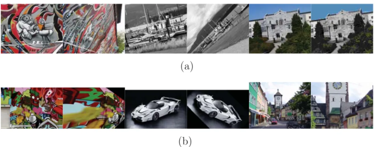
nonlinear). Some examples of each dataset used for evaluation are illustrated in Figure 2.2.
2.5.2
Evaluation Criteria
The criteria employed to measure the performance of the salient point methods in each application are summarized in Table 2.2. We follow the commonly used
2.6 Results and Discussions
(a)
(b)
Figure 2.2: Examples from each dataset for the evaluation of salient point meth-ods. (a) Examples from the Oxford dataset [108] used for the evaluation of the accuracy of correspondence matching. (b) Examples from the Fischer dataset [121] used for the evaluation of the accuracy of correspondence matching.
Table 2.2: Overview of the evaluation criteria used in the experiments.
Criteria Function description
Repeatability [107]
Measures the performance of the detector: the higher the repeatability score, the bet-ter the performance.
Recall and precision [108]
Measures the accuracy of correspondence matches: a distinctive descriptor shows high recall at any precision.
Number of correct correspondences
Total amount of correct correspondences between two compared images, a robust method shows a high score.
2.6
Results and Discussions
2.6.1
Detector Evaluation
0.1 0.2 0.3 0.4 0.5 0.6 1-Overlap error 0 0.1 0.2 0.3 0.4 0.5 0.6 0.7 Repeatability Oxford Dataset SIFT SURF ORB BRISK FAST CenSurE GFTT MSER Hessian-Affine KAZE
0.1 0.2 0.3 0.4 0.5 0.6
1-Overlap error 0 0.1 0.2 0.3 0.4 0.5 0.6 0.7 Repeatability Fisher Dataset SIFT SURF ORB BRISK FAST CenSurE GFTT MSER Hessian-Affine KAZE
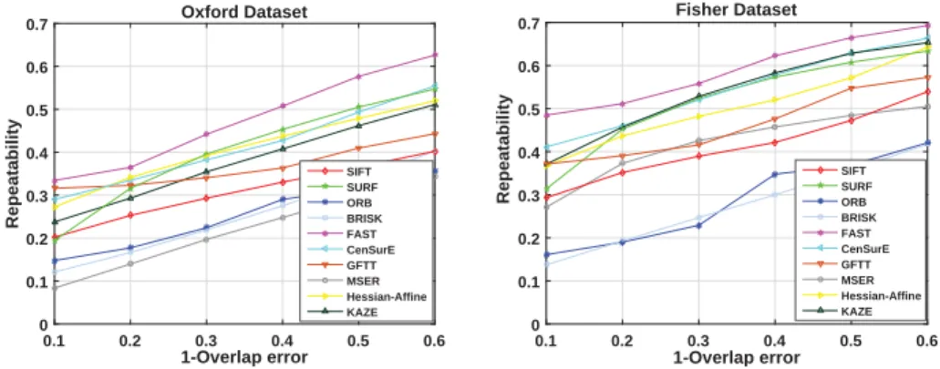
Figure 2.3: The performance evaluation of salient point detectors based on the criterion of repeatability.
KAZE, MSER and Hessian-Affine.
An important evaluation criterion from the research literature is repeatability [107]. The repeatability score is calculated as the ratio between the number of
correspondences and the minimum ofm1 andm2, wherem1,m2 denote the
num-ber of points in the reference and the query images after projecting the reference image points by the ground truth homography and discarding those points outside the common area, respectively.
repeatability = C(m1, m2)
min(m1, m2) (2.3)
C(m1, m2) is the number of correspondences between m1 and m2. An overlap
error is used to identify the correspondence. For a keypoint region in the query image which is the nearest one to a projection keypoint region in the reference image by using homography: if the ratio between the intersection of the two regions and the union of the two regions is larger than the overlap error, it will be considered as a correspondence. We compute the average repeatability scores on the whole dataset, respectively, thus, the detection performance of each method can be estimated in a comprehensive perspective. The trend of average repeatability under varying overlap errors (in the range from 0.4 to 0.9) is shown in Figure 2.3.
2.6 Results and Discussions
the repeatability scores is clearly indicated when the value of 1-overlap error becomes larger. We can also notice that the FAST detector had the highest repeatability and the ORB and BRISK detectors obtained the lowest scores. The detectors SURF, Hessian-Affine, KAZE, and CenSurE have a similar rank on
both datasets. The performance of the nonlinear scale space detector KAZE reveals superior results to the well known SIFT detector. All detectors can reach a stable and acceptable performance when the value of overlap error is 0.5, so the
overlap error will be set at 0.5 to identify the correspondences in the following experiments.
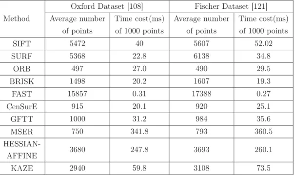
Since the salient point detection mechanism in each salient point method is based on a different scheme, which results in a different computational complexity, and a different set of feature points can be extracted from the same image, time
costs should be compared statistically. We applied different types of detectors to various test images, in order to determine statistically significant results. The average number of detected points and the time cost of the compared salient point
methods are shown in Table 2.3.
Table 2.3: Comparison of average number of detected points and detection time
Method
Oxford Dataset [108] Fischer Dataset [121]
Average number Time cost(ms) Average number Time cost(ms)
of points of 1000 points of points of 1000 points
SIFT 5472 40 5607 52.02
SURF 5368 22.8 6138 34.8
ORB 497 27.0 490 29.5
BRISK 1498 20.2 1607 19.3
FAST 15857 0.31 17388 0.27
CenSurE 915 20.1 920 25.1
GFTT 1000 31.2 984 35.6
MSER 750 341.8 793 360.5
HESSIAN-AFFINE 3680 247.8 3693 260.1
The results listed in Table 2.3 reveal that the most efficient detector is FAST. FAST detected the largest number of salient points on both datasets, which is almost ten times higher than what was obtained by other detectors. FAST defines the salient points according to simple intensity comparisons, thus, the time cost
is only 0.31 ms for a total of 15857 points on the Oxford dataset [108] and 0.27 ms for 17388 points on the Fischer dataset [121]. The most time-consuming detectors are MSER and Hessian-Affine, because they need do the ellipse fitting for each salient point. The detectors SIFT, SURF, ORB, BRISK and KAZE
all contain scale space and rotation estimation procedures. KAZE builds the nonlinear scale space in an iterative way using the AOS scheme which is much more time consuming than the linear scale space calculation. As SURF, ORB
and BRISK speed up building the scale space, they are more efficient than the SIFT detector.
2.6.2
Descriptor Evaluation
The Oxford and Fischer datasets are also utilized in the local descriptors evalua-tion. Note that some of the salient point detectors from the previous section do not define descriptors and are not compared here. In order to make an objective comparison of different salient point descriptors, SURF was applied as the salient
point detector, as the SURF detector is scale invariant and it provides a high repeatability score according to its performance in the detector evaluation. We combined SURF detectors with local descriptors including SIFT, SURF, ORB,
BRIEF, BRISK, FREAK, BinBoost and LATCH. The evaluation starts by ex-tracting salient point features from the reference images and establishing a KD-tree or LSH index space for the obtained local features. Then, we extract features from the query image and match them against the features from each reference
2.6 Results and Discussions
The NNDR is used as the matching strategy to find similar descriptors in
im-age pairs. In addition we use recall and 1-precision [108] (not to be confused with precision@1) as criteria to measure the performance of various salient point descriptors. Recall denotes the number of correct matches with respect to the number of correspondences between two compared images, and the precision is the number of correct matches with respect to the total number of matches.
recall= #correct_matches
#correspondences (2.4)
precision= #correct_matches
#total_matches (2.5)
We varied the value of the threshold in the NNDR to obtain the curves of the
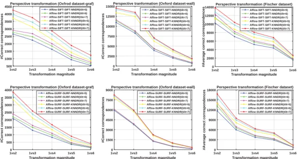
tendency of the average recall vs. 1-precision under each transformation. Figure 2.4 and Figure 2.5 show the results on each dataset. We also provide the area under the recall vs. 1-precision curve, averaged over all image transformations in each dataset, as shown in Table 2.4 and Table 2.5. A distinctive descriptor would give a high score of area under each curve (AUC).
0 0.1 0.2 0.3 0.4 0.5 0.6 0.7 0.8 0.9 1 1-precision 0 0.1 0.2 0.3 0.4 0.5 0.6 0.7 0.8 0.9 1 Recall Affine transformation SIFT SURF ORB BRISK BRIEF FREAK BinBoost LATCH
0 0.1 0.2 0.3 0.4 0.5 0.6 0.7 0.8 0.9 1 1-precision 0 0.1 0.2 0.3 0.4 0.5 0.6 0.7 0.8 0.9 1 Recall Image blur SIFT SURF ORB BRISK BRIEF FREAK BinBoost LATCH
0 0.1 0.2 0.3 0.4 0.5 0.6 0.7 0.8 0.9 1 1-precision 0 0.1 0.2 0.3 0.4 0.5 0.6 0.7 0.8 0.9 1 Recall Illumination SIFT SURF ORB BRISK BRIEF FREAK BinBoost LATCH
0 0.1 0.2 0.3 0.4 0.5 0.6 0.7 0.8 0.9 1 1-precision 0 0.1 0.2 0.3 0.4 0.5 0.6 0.7 0.8 0.9 1 Recall JPEG compression SIFT SURF ORB BRISK BRIEF FREAK BinBoost LATCH
Figure 2.4: Comparison of various descriptors using recall vs 1-precision under different image degradations. The evaluation results are for the Oxford dataset [108].
has a big influence on the SURF descriptor, while the other descriptors are ro-bust to illumination changes and show scores close to each other. The evaluation results on the Fischer dataset [121] show the same tendency under the changes of image blur and perspective when compared to the results on the Oxford dataset [108]. In addition, the descriptors of ORB, BRIEF and LATCH also show their weakness under the change of image zoom.


![Table 2.4: The Oxford benchmark results [108]. Numerical results summarizing area under the recall vs](https://thumb-us.123doks.com/thumbv2/123dok_us/8257182.2187691/49.892.189.645.872.1098/table-oxford-benchmark-results-numerical-results-summarizing-recall.webp)