5079.pdf

(1)

Entropy of Transformations that Preserve an Infinite Measure

Rachel Louise Bayless

A dissertation submitted to the faculty of the University of North Carolina at Chapel Hill in partial fulfillment of the requirements for the degree of Doctor of Philosophy in the Department of Mathematics.

Chapel Hill 2013

Approved by:

Jane Hawkins Karl Petersen Hans Christianson

(2)

Abstract

RACHEL LOUISE BAYLESS: Entropy of Transformations that Preserve an Infinite Measure

(Under the direction of Jane Hawkins)

(3)

Acknowledgments

I would like to briefly thank those who have supported me both personally and professionally through this long process. In particular, I would like to thank my advisor, Jane Hawkins, for her helpful guidance and encouragement. I sincerely ap-preciate the time and effort that she invested in my success. Additionally, I would like to thank Karl Petersen, Hans Christianson, Sue Goodman, and Joseph Plante for serving on my committee. I very much appreciate their insightful comments and suggestions.

(4)

List of Figures

2.1. How the atoms of A and Bmove under T. . . 9

4.1. An example ofS when N = 4. . . 37

4.2. An example of conjugated S when N = 4. . . 43

4.3. An example of the Qpartition for S when N = 4. . . 44

5.1. How hitting-time sets move under ψj, j = 1, ..., N + 1. . . 69

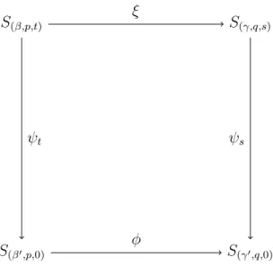
6.1. A commutative diagram of 1-isomorphisms. . . 92

(7)

CHAPTER 1

INTRODUCTION

In this dissertation we study the dynamics of transformations that preserve an infinite measure. In particular, we investigate the measure-theoretic properties of rational functions which preserve Lebesgue measure on the real line. While the liter-ature on measure-theoretic properties of finite-measure-preserving transformations is well elaborated, there is not always a clear analogue of these properties for infinite-measure-preserving systems. In particular, entropy does not have a clear extension to transformations that preserve an infinite measure. The entropy of a system measures the amount of information gained with each application of an experiment or transfor-mation. Higher entropy corresponds to more disorder and less predictable systems. The classical Kolmogorov-Sinai definition of entropy relies heavily on the ability to associate probabilities to possible events or outcomes. Thus, there is no universal analogue of entropy for infinite-measure-preserving systems. Different possibilities have been given independently by Krengel [Kre], Parry [Par], and Roy [Roy]. Two of these definitions have been around since the late 1960’s, but there exist very few examples where any of these entropies have been computed explicitly. In this disser-tation we provide a method of computing the Krengel entropy for an entire class of rational maps which preserve Lebesgue measure on the real line. Furthermore, we prove that these transformations are quasi-finite, so the three definitions of Krengel, Parry, and Roy coincide.

The transformations of interest in this thesis are a negative variant ofR-functions. An R-function is an analytic map on the upper-half plane, _R2+ ₌_{_x₊_iy _: _{y >}_0},

(8)

various names including Herglotz functions or Nevanlinna functions. The name R -function, however, dates back to Kac and Krein [KK]. No single source provides a complete history of R-functions, so in Chapter 3 we give a detailed description of the context in which such functions arise. This work is primarily concerned with dynamics of one-dimensional maps, so we impose an extra condition on R-functions. Given an R-function, f, we require that for Lebesgue almost every x ∈ _R, we have limy→0f(x+iy) =F(x), whereF :R→Ris a measurable map. Such maps F which are called the boundary functions associated to R-functions.

This dissertation provides an in depth study of the boundary functions associated to rational R-functions of negative type. These are rational maps, T : _R → _R such that T = −F, where F is the boundary function associated to an R-function to _R. In [Let] Letac proved that all rational R-functions (of both positive and negative type) preserve Lebesgue measure. Furthermore, the measure-theoretic properties of

R-functions of positive type have been studied by Aaronson in [Aar2].

In Chapter 2 we give a brief introduction to classical measure-theoretic dynamical properties such as conservativity, ergodicity, and exactness. We also detail some nonstandard properties which arise only when considering infinite-measure-preserving systems. These properties are rational ergodicity and pointwise dual ergodicity. In Chapter 3 we give an overview of Aaronson’s results on R-functions of positive type to provide context for our work on the negative case.

In Chapter 4 we prove that all rational R-functions of negative type are conser-vative, exact, and ergodic with respect to Lebesgue measure. We further prove that all rational R-functions of negative type are rationally ergodic and pointwise dual er-godic. These results are less restrictive than the aforementioned results of Aaronson for R-functions of positive type.

(9)

measure. Furthermore, in Chapter 4 we show that all rationalR-functions of negative type are quasi-finite, which implies that the three definitions of entropy coincide.

The usefulness of entropy in ergodic theory arises from the fact that it is an isomorphism invariant. That is, if two probability-preserving transformations are iso-morphic, then they have the same entropy. For infinite-measure-preserving systems, however, there exist less restrictive isomorphisms called c-isomorphisms. In fact, if two infinite-measure-preserving transformations are c-isomorphic where c 6= 1, then they do not necessarily have the same Krengel entropy. In Chapter 6 we provide complete invariants (involving entropy) for c-isomorphisms between quadratic ratio-nal R-functions of negative type. We also give preliminary results on 1-isomorphism invariants for cubic rational R-functions of negative type.

(10)

CHAPTER 2

BACKGROUND

2.1. Preliminary Definitions

We begin with a few basic definitions of classical properties in ergodic theory. We use (X,B, m) to denote a measure spaceX together with a σ-algebra of measurable sets, B, for a measure, m. We assume throughout that the measure m is σ-finite. We use (X,B, m, T) to denote a σ-finite measure space (X,B, m) together with a transformation T : X → X such that T−1B ⊆ B. In this dissertation we consider only nonsingular systems (X,B, m, T). That is, given A∈ B, we have m(T−1A) = 0 if and only if m(A) = 0. In fact, we are primarily interested in measure-preserving transformations (defined below) which is stronger than nonsingular.

Definition 2.1.1. A measurable function T : (X,B, m) → (X,B, m) is called

measure-preserving if m(T−1A) = m(A) for all A∈ B.

We study the dynamical properties of measure-preserving transformations. In particular, we focus on transformations which preserve an infinite measure. That is, we consider measure-preserving systems (X,B, m, T) such that m(X) = ∞. We call such systems infinite-measure-preserving. A few of the most commonly studied measure-theoretic properties are defined below.

Definition2.1.2. A nonsingular system (X,B, m, T) isergodicif for everyA∈ B

(11)

In other words, T is ergodic if the only invariant sets are trivial or the entire space. The next property also involves the preimages of sets and is closely related to ergodicity.

Definition 2.1.3. A nonsingular system (X,B, m, T) is exact if

(2.1.1) ∩n>0T−nB={∅, X} mod m.

Equivalently, a nonsingular system (X,B, m, T) is exact if A∈ B such that

(2.1.2) T−n(Tn(A)) =A for all n >0,

implies m(A) = 0 orm(Ac) = 0.

The following classical result can be found in [Roh2], and is given here for com-pleteness.

Lemma 2.1.4. Let T be a nonsingular transformation of (X,B, m). If T is exact,

then T is ergodic.

In general the converse of Lemma 2.1.4 does not hold. For example, if T is invertible, then T is not exact. Furthermore, Eigen and Hawkins have constructed noninvertible shift maps which are ergodic but not exact (see [EH]).

Another classical property of interest is related to the recurrence of points to positive measure sets.

Definition 2.1.5. A set A ∈ B is called wandering for the nonsingular system

(X,B, m, T) if the sets{T−i_A_}∞

i=0 are pairwise disjoint.

Definition 2.1.6. A nonsingular system (X,B, m, T) is called conservative if

there does not exist a wandering set of positive measure.

(12)

and m(T−1A) = m(A), then A only has so much room to “wander” throughout a finite space X. On the other hand, if m(X) = ∞, then conservativity of T is not automatic, because the inverse images of A won’t necessarily fill the entire infinite space. Conservativity is, however, tied to the existence of measurable sets which do sweep out the entire space X.

Definition 2.1.7. Let (X,B, m, T) be a nonsingular system. A set A ∈ B is

called asweep-out set for T if

(2.1.3)

∞

[

n=0

T−nA=X mod m.

Equivalently, A is a sweep-out set if for almost every x ∈X there exists an nx such that Tnx₍_x₎_∈_A_.

The following theorem relates the existence of sweep-out sets to conservativity of measure-preserving transformations.

Theorem2.1.8 (Maharam’s Recurrence Theorem, [Mah]). Suppose(X,B, m, T)

is a measure-preserving system. If there exists a sweep-out setA∈ Bwithm(A)<∞, then T is conservative.

Finally, we introduce the notion of an isomorphism between measure-preserving transformations.

Definition 2.1.9 (Isomorphic). Let (X1,B1, m1, T1) and (X2,B2, m2, T2) be two

measure-preserving systems. Suppose we have two sets M1 ∈ B1 and M2 ∈ B2 with

m1(X1\M1) = 0 and m2(X2 \M2) = 0 such that T1(M1) ⊆M1 and T2(M2)⊆ M2.

We say (X1,B1, m1, T1) is isomorphic to (X2,B2, m2, T2) (or T1 is isomorphic to T2)

if there exists an invertible mapφ :M1 →M2 such that for allA ∈ B2|M2,

(1) φ−1(A)∈ B1|M1,

(13)

(3) (φ◦T1)(x) = (T2◦φ)(x) for all x∈M1.

We will denote this situation by φ:T1 →T2, and φ is called an isomorphism.

It is clear that measure-theoretic properties such as conservativity, exactness, and ergodicity are invariant under isomorphism.

2.2. The Induced Transformation and Return-Time Sets

As stated above, we are primarily interested in studying measure-theoretic prop-erties of transformations preserving an infinite measure. One technique that will be used throughout the following sections is inducing on a set of finite measure. The induced transformation provides a way to study the dynamics of transformations that preserve an infinite measure by looking only at a finite piece of the space.

Let (X,B, m, T) be a nonsingular system. Given A ∈ B let ˜A ⊆ A be the set defined by ˜A =T∞

n=1

S∞

i=nT

−i_A_{. That is, ˜}_A _{is the set of points in} _X _{which “hit”} _A infinitely often under iteration of T. For x∈A˜ define φA(x) = min{n : Tn(x)∈A}. That is,φA(x) is thefirst-hitting-time ofxtoA. Ifx∈A, thenφA(x) is often referred to as the first-return-time of x to A. The induced transformation, TA : A → A, is defined by

TA(x) = TφA(x)(x) forx∈A˜

TA(x) = xfor x /∈A.˜

We note that if T is a conservative transformation and A is a sweep-out set for

T, then by Definition 2.1.7 we have A = ˜A. Letting B|A = {B ∩A : B ∈ B} and

m|A(B) =m(A∩B), we have the following classical result.

Theorem 2.2.1. Suppose (X,B, m, T) is a measure-preserving system. If A is a

(14)

If (X,B, m, T) is an infinite-measure-preserving system and A is a sweep-out set with m(A) < ∞, then inducing on A yields a finite-measure-preserving sys-tem (A,B|A, m|A, TA). We can often deduce information about the original infinite-measure-preserving system, (X,B, m, T), from the dynamics of the finite-measure-preserving system (A,B|A, m|A, TA). For example, we have the following classical theorem which can be found in [AW].

Theorem 2.2.2. If (A,B|A, m|A, TA) is ergodic, then(X,B, m, T) is also ergodic.

In subsequent sections we will discuss similar results for studying the behavior of (X,B, m, T) via (A,B|A, m|A, TA). Thus, it is important to know when sweep-out sets exist for infinite-measure-preserving systems. The following theorem says that if (X,B, m, T) is conservative and ergodic, then every positive-measure set is a sweep-out set.

Theorem 2.2.3. Let (X,B, m, T) be an infinite-measure-preserving system. If T

is conservative and ergodic, then every A∈ B such that m(A)>0 is a sweep-out set for T.

Proof. Let A∈ B such that m(A)>0. Set

(2.2.1) CA={x∈X:

∞

X

n=1

(1A◦Tn)(x) =∞}.

We have that CA is invariant forT. Therefore, by ergodicity,m(CA) = 0 or m(CAc) = 0. However, by conservativity of T, we have that A⊆CA, so CA=X mod m. That is, almost everyx∈Xhits Ainfinitely often under iteration ofT, soAis a sweep-out

set.

(15)

LetA denote the first-return partition of A. That is, A={Ak}, where

(2.2.2) Ak ={x∈A:φA(x) =k}=A∩T−kA\ k−1

[

j=1

T−jA.

LetB={Bk} be a similar partition of Ac. That is,

(2.2.3) Bk ={x∈Ac:φA(x) = k}=Ac∩T−kA\ k−1

[

j=1

T−jA=T−kA\ k−1

[

j=0

T−jA.

It is useful to view the action of T on the sets Ak and Bk as a two-story tower (see Figure 2.1).

B1 B2 B3 ...

A1 A2 A3 A4 ...

A

Ac

A

Figure 2.1. How the atoms of Aand B move under T.

We now further develop the notation and make a few observations that will be helpful in subsequent sections. We define another collection of sets{Dn}n≥0by setting

(2.2.4) D0 =A and Dn={x∈A:φA(x)> n} for n≥1.

We note that Dn = ∪∞k=n+1Ak and the {Dn}n≥0 are nested such that Dn+1 ⊂ Dn. Furthermore, we can relateDn and Bn via the following result.

Lemma2.2.4. Let(X,B, m, T)be a conservative, ergodic, measure-preserving

sys-tem. Given the sets {Dn}n≥0 and {Bn}n≥1 defined as above we have

(16)

Proof. By the definition of {An}and {Dn}we have

(2.2.6) m(A) =m

n

[

k=1

Ak

!

+m

∞

[

k=n+1

Ak

!

= n

X

k=1

m(Ak) +m(Dn).

We also have

(2.2.7) T−1A= (T−1A∩A)∪(T−1A\A) =A1∪B1.

Therefore, (2.2.8)

T−2A=T−1A1∪T−1B1 =T−1A1∪(T−1B1∩A)∪(T−1B1\A) =T−1A1∪A2∪B2.

Thus, repeated application of (2.2.7) yields

(2.2.9) T−nA=T−(n−1)A1∪T−(n−2)A2∪...∪T−1An−1∪An∪Bn,

which is a disjoint union. By assumption m is an invariant measure for T, so

m(T−nA) = m

_n [

k=1

T−(n−k)Ak

!

∪Bn

!

= n

X

k=1

m(T−(n−k)Ak) +m(Bn)

= n

X

k=1

m(Ak) +m(Bn)

= n

X

k=1

m(Ak) +m(Dn)

= m(A),

where the last two lines come from the definition ofDnand the observation in (2.2.6).

(17)

of entropy in Chapter 5. The statement can be found in [Yur], however no proof is given there.

Lemma 2.2.5. Let (X,B, m, T) be a nonsingular system. Let A ∈ B with 0 < m(A) <∞ be a sweep-out set, and suppose νA << m|A is a TA-invariant measure. Then the following formula gives a T-invariant measure µνA << m:

(2.2.10) µνA(E) = ∞

X

k=0

νA(Dk∩T−kE), for all E ∈ B.

Proof. Given E ∈ B, we have

µνA(E) = ∞

X

k=0

νA(Dk∪T−kE) =

∞

X

k=0

Z

Dk

1(T−k_E₎dν_A.

Therefore,

µνA(T −1

E) =

∞

X

k=0

νA(Dk∩T−(k+1)E) =

∞

X

k=0

Z

Dk

1(T−(k+1)_E₎dν_A

= ∞ X k=1 ∞ X

j=k

Z

Aj

1(T−k_E₎dν_A

= ∞ X k=1 Z Ak

1(T−k_E₎dν_A+ ∞

X

k=2 ∞

X

j=k

Z

Aj

1(T−k_E₎dν_A

= νA(TA−1(A∩E)) +

∞

X

k=1

Z

Dk

1(T−k_E₎dν_A.

(2.2.11)

The measureνA is invariant for TA, so we haveνA(TA−1(A∩E)) =νA(A∩E). Thus, (2.2.11) becomes

(2.2.12) νA(A∩E) +

∞

X

k=1

Z

Dk

1(T−k_E₎dν_A = ∞

X

k=0

Z

Dk

1(T−k_E₎dν_A=µ_ν A(E).

(18)

Lemma 2.2.6. If A is a sweep-out set, and µ|A isTA invariant, then µµ|A =µ.

Proof. Given n ≥0 and E ∈ B, we have

(2.2.13) µ(E) =µ|A(A∩E) + n

X

k=1

µ|A(Dk∩T−kE) +µ

_n [

k=0

T−kA

!c

∩T−nE

!

.

Since A is a sweep-out set we know limn→∞µ Sn_k₌₀T−kA

c

= 0, so

(2.2.14) µ(E) = µ|A(A∩E) +

∞

X

k=1

µ|A(Dk∩T−kE) =µµ|A(E).

2.3. The Perron-Frobenius Operator

In this section we develop a few more tools for studying the behavior of dynamical systems which will be used in subsequent sections. We say a nonsingular system (X,B, m, T) is n-to-1 if for almost every x ∈ X, the set T−1(x) contains precisely n

distinct points. Given a nonsingular, n-to-1 system (X,B, m, T), we call a partition P ={Pi}n

i=1 of X a Rohlin partition for T if T :Pi → X is one-to-one and onto for each i= 1, ..., n (see [Roh1]). Furthermore, we denote each branch T|Pi by Ti.

Definition 2.3.1. Let (X,B, m, T) be a nonsingular n-to-1 system, and letP =

{Pi}ni=1 be a Rohlin partition of X. We define the Jacobian of T by

(2.3.1) JT(x) =

n

X

i=1

1Pi(x)

dmTi

dm (x).

We note that if X = _R, m is Lebesgue measure, and T is piecewise C1, then

JT(x) = |T0(x)|.

Definition2.3.2. Given a nonsingularn-to-1 system (X,B, m, T) andf ∈L1(m),

we define the Perron-Frobenius operator by

(2.3.2) LTf(x) =

X

y∈T−1₍_x₎ f(y)

JT(y)

(19)

Given a nonsingular n-to-1 system (X,B, m, T) and a Rohlin partition P = {Pi}ni=1 we let ψi denote the inverse of T restricted to Pi. Therefore, ψi = Ti−1 :

X → Pi is a one-to-one and onto mapping. We can rewrite (2.3.2) as LTf(x) =

Pn

i=1

f(ψi(x))

JT(ψi(x)). We note that T(T

−1₍_x_{)) =} _x _{for all} _x _∈ _X_{, so} _T₍_ψ

i(x)) = x for all

i= 1, .., nandx∈X. Taking the Jacobian of both sides yieldsJT(ψi(x))·Jψi(x) = 1.

Therefore, Jψi(x) = 1

JT(ψi(x)). Therefore, for f ∈ L

1₍_m_{) equation (2.3.2) can be}

rewritten as

(2.3.3) LTf(x) =

n

X

i=1

f(ψi(x))·Jψi(x).

The following lemma relates the Perron-Frobenius operator to the existence of an invariant measure for T and can be found in [Haw].

Lemma 2.3.3. Given a nonsingular n-to-1 system (X,B, m, T), a function f ∈ L1₍_m₎_satisfies_L

Tf =f if and only if the measureν defined byf dm=dν is invariant for T.

Proof. Suppose f ∈ L1(m) such that LT(f) = f and ν is a measure on X defined by f dm=dν. For A∈ B we have

(2.3.4) ν(A) =

Z

X

1A(x)dν(x) =

Z

X

1A(x)·f(x)dm(x) =

Z

X

1A(x)·(LTf)(x)dm(x).

By the definition of LT in (2.3.3) we have that (2.3.4) is equal to

(2.3.5)

Z

X

1A(x)· n

X

i=1

f(ψi(x))·Jψi(x)dm(x).

We let ψi(x) =y, so the above line becomes

(2.3.6)

Z

X n

X

i=1

1ψiA(y)·f(y)dm(y) =

Z

X

1T−1_Af(y)dm(y) = ν(T−1(A)).

(20)

Another well-studied operator that is related to the Perron-Frobenius operator is the Koopman operator.

Definition 2.3.4. Given f ∈Lp(m), the Koopman operator is defined by

(2.3.7) UT(f)(x) = (f ◦T)(x).

It is well known that UT : Lp(m) → Lp(m) is a linear isometry, but for our purposes we will restrict to the case where p=∞. From functional analysis we have that the dual of L1₍_m_{) is} _L∞₍_m_{). The dual pairing} _h·_,_·i _: _L1₍_m₎_×_L∞₍_m₎ _→

R satisfies

(2.3.8) hf, gi=

Z

X

f(x)·g(x)dm(x), for (f, g)∈L1(m)×L∞(m).

Now letting (f, g) ∈ L1(m)×L∞(m) and considering the operators LT and UT, we have

(2.3.9) hLTf, gi=

Z

X

(LTf)(x)·g(x)dm(x) =

Z

X n

X

i=1

f(ψi(x))·Jψi(x)·g(x)dm(x).

We change variables setting y=ψi(x), and (2.3.9) becomes

(2.3.10) n

X

i=1

Z

ψi(X)

f(y)·(g◦T)(y)dm(y) =

Z

X

f(y)·(g◦T)(y)dm(y) =hf, UTgi.

Therefore, the Perron-Frobenius operator is dual to the Koopman operator, and LT is often referred to as the dual operator (as in [Aar4]). We adopt this language in the subsequent sections.

2.4. Rational Ergodicity and Pointwise Dual Ergodicity

(21)

Theorem 2.4.1. Suppose (X,B, m, T) is a system preserving a σ-finite measure,

and let f ∈L1(m). Then

(2.4.1) lim

n→∞

1

n

n−1

X

i=0

f(Tix) = f∗ almost everywhere,

where f∗ ∈L1₍_m_{). Furthermore,} _f∗_◦_T ₌_f∗ _{almost everywhere.}

We are interested in studying “Birkhoff-like” properties for ergodic transforma-tions preserving an infinite measure. Two such properties are called rational ergodici-tiy and pointwise dual ergodicity. Both definitions are due to Aaronson and have been studied in [Aar1], [Aar2], and [Aar4]. These are nonstandard notions, and no single source gives their entire story (including motivation, definition, and relationship to each other). Thus, we give a complete description here.

2.4.1. Rational Ergodicity. If (X,B, m, T) is an ergodic finite-measure-preserving system, then we have the following consequence of the Birkhoff ergodic theorem. If

A, B ∈ B, then

(2.4.2) lim

n→∞

1

n

n−1

X

k=0

m(B∩T−kA) = m(A)m(B)

m(X) .

On the other hand, if m(X) =∞, then (2.4.2) is not well defined. We are interested in properties in the flavor of (2.4.2) that are satisfied by transformations preserving an infinite measure.

LetA ∈ B with 0< m(A)<∞, and let an(A) =

Pn−1

k=0m(A∩T

−k_A_{). Let} _W₍_T₎ denote the collection of sets, A∈ B, satisfying

(2.4.3) lim

n→∞

1

an(A) n−1

X

k=0

m(B ∩T−kC) = m(B)m(C)

m(A)2 ,

for all B, C ∈ B ∩A. We say that T is weakly rationally ergodic if T is ergodic and

(22)

We now introduce a stronger condition than weak rational ergodicity. Let R(T) denote the collection of sets for which

(2.4.4) sup

n≥1

Z

A 1

an(A) n−1

X

k=1

1A◦Tk

!2

dm <∞.

We say that T is rationally ergodic if T is ergodic and R(T) 6= ∅. We will show that rational ergodicity implies weak rational ergodicity. First, we must catalogue the following well-known property of Hilbert spaces. A proof can be found in most functional analysis text books (see for example [Wei]).

Theorem 2.4.2. Let H be a Hilbert space. Every bounded sequence (fn) in H contains a weakly convergent subsequence (fnk).

Using Theorem 2.4.2 we prove the following lemma, which was originally stated in [Aar1]. Recall from Section 2.2 that TA denotes the induced transformation and

φA(x) denotes the first-return-time of x toA.

Lemma 2.4.3. Let A ∈ R(T) and ωn = (1/an(A))

Pn−1

k=01A ◦Tk. Then, there

exists a subsequence such that ωnk →ω weakly in L

2₍_A₎ _and _ω_◦_T

A=ω.

Proof. Let A ∈ R(T) and ωn = (1/an(A))

Pn−1

k=01A ◦T

k _{be as above. Then,} by (2.4.4) for all n ≥ 1 we have ωn ∈ L2(A) and there exists an M such that ||ωn||2 ≤ M. Thus, by Theorem 2.4.2 there exists a subsequence of ωnk of ωn such

that ωnk → ω weakly in L

2₍_A_{). We abuse notation and write} _ω

(23)

(ωn◦TA)(x) = 1

an(A) n−1

X

k=0

1A(Tk(TA(x)))

= 1

an(A) n−1

X

k=0

1A(Tk+φA(x)(x))

= 1

an(A)

n−1+φA(x)

X

k=φA(x)

1A(Tk(x))

= 1

an(A)





n−1+φA(x)

X

k=0

1A(Tk(x))−

φA(x)−1

X

k=1

1A(Tk(x))−1A(x)





The middle term PφA(x)−1

k=1 1A(Tk(x)) = 0 since Tk ∈/ A for all 1 ≤ k ≤ φA(x)−1. Also,x∈A, so 1A(x) = 1. Thus, we have,

(ωn◦TA)(x) =ωn+φA(x)(x)−

1

an(A)

.

Taking the limit of both sides we see that ω◦TA =ω almost everywhere.

Before proving that rational ergodicity is indeed stronger than weak rational er-godicity we make one final note about eachωn. We have

Z

A

ωndm = 1

an(A)

Z

A n−1

X

k=0

1A◦Tk

= 1

an(A) n−1

X

k=0

m(A∩T−kA) = 1.

Thus, we have that R

Aωndm= 1 ∀n.

Theorem 2.4.4. If an ergodic measure-preserving system, (X,B, m, T), is

ratio-nally ergodic, then it is weakly ratioratio-nally ergodic.

Proof. We will show that R(T) ⊆ W(T). Let A ∈ R(T), and let ωn = (1/an(A))

Pn−1

k=01A◦T

k_{. By Lemma 2.4.3 we have} _ω_◦_T

A=ω, and the ergodicity of

TAimplies thatωis constant a.e. We also know that

R

Aωndm = 1∀n, so

R

(24)

Thus, we have that ω = 1/m(A) almost everywhere. Further, if B ∈ B ∩A, then

R

Bωn →

R

Bω. Integrating we see that

(2.4.5) 1

an(A) n−1

X

k=0

m(B∩T−kA)→ m(B)

m(A) for all B ∈ B ∩A.

The same argument applies to T−1 since T is measure-preserving, so

(2.4.6) 1

an(A) n−1

X

k=0

m(A∩T−kB)→ m(B)

m(A) for all B ∈ B ∩A.

Now choose any C ∈ B ∩A and let σn = (1/an(A))Pn

−1

k=01C ◦T

k_{, then} _||_σ

n||2 ≤M,

for n ≥ 1. An argument similar to that in the proof of Lemma 2.4.3 shows that

R

Aσn→

R

Aσ, and σ is constant almost everywhere. Integrating σn overA we obtain

Z

A

σndm = 1

an(A)

Z

A n−1

X

k=0

1C ◦Tkdm

= 1

an(A) n−1

X

k=0

m(T−kC∩A).

Thus, by (2.4.6) we have R_Aσndm→ m_m(₍C_A)₎, so

(2.4.7) σn→

m(C)

m(A)2.

In particular, integrating both sides of (2.4.7) over B ∈ B ∩A yields

(2.4.8) 1

an(A) n−1

X

k=0

m(B∩T−kC)→ m(B)m(C)

m(A)2 .

(25)

2.4.2. Pointwise Dual Ergodicity. Now, we turn our attention to another prop-erty of ergodic transformations preserving an infinite measure. We have the following consequence of the Birkhoff ergodic theorem (Theorem 2.4.1). If T is ergodic and

m(X)<∞, then

(2.4.9) lim

n→∞

1

n

n−1

X

i=0

f(Tix) = 1

m(X)

Z

f dm,

almost everywhere for allf ∈L1₍_m_{). Again, (2.4.9) holds only if}_m₍_X₎_<_{∞. We are}

interested in a property in the flavor of (2.4.9) that is well defined when m(X) =∞. We now state the definition of a pointwise dual ergodic transformation, which is a system preserving aσ-finite measure that has a “Birkhoff-like” property.

Definition 2.4.5. A conservative, ergodic, infinite-measure-preserving system

(X,B, m, T) is called pointwise dual ergodic if there are constants an(T) such that

lim n→∞

1

an(T) n−1

X

k=0

Lk

Tf(x) =

Z

X

f dm,

almost everywhere for all f ∈L1₍_m_).

Aaronson proved the following theorem which shows pointwise dual ergodicity is stronger than rational ergodicity.

Theorem 2.4.6 ([Aar4]). Let (X,B, m, T) be a conservative ergodic

measure-preserving system. If T is pointwise dual ergodic, then T is rationally ergodic.

In order to study infinite-measure-preserving transformations, we often study the transformation on a finite piece of the space. Thus, in infinite ergodic theory we are often interested in the existence of particularly nice sets called Darling-Kac sets.

Definition2.4.7. Let (X,B, m, T) be a conservative, ergodic, measure-preserving

(26)

exist constants an(A)>0 such that

(2.4.10) 1

an(A) n−1

X

k=0

Lk

T1A →1 uniformly for almost every x∈A.

We will draw a connection between Darling-Kac sets and pointwise dual ergodic transformations (and thereforean(A) andan(T)) via Hurewicz’s ergodic theorem. For completeness, we state Hurewicz’s ergodic theorem here.

Theorem2.4.8 (Hurewicz’s Ergodic Theorem, [Hur]). Suppose that(X,B, m, T)

is a conservative, ergodic, nonsingular system. Then, for all f, g ∈L1₍_m₎ _{we have}

(2.4.11) lim

n→∞

Pn

k=1L

k Tf(x)

Pn

k=1L

k Tg(x)

=

R

Xf dm

R

Xgdm

for almost every x∈X.

It is well known that if a conservative, ergodic, measure-preserving transforma-tion T has Darling-Kac sets, then it is pointwise dual ergodic ([Aar4]). This result follows from Hurewicz’s ergodic theorem letting g = 1A and an(T) =

an(A)

m(A), where

A is a Darling-Kac set. Another consequence of Hurewicz’s ergodic theorem is the asymptotic universality of an(T).

Definition 2.4.9. Given two sequences{an} and {bn} of real numbers we write

(2.4.12) an∼bn, if lim

n→∞

an

bn = 1.

In this case we say {an} is asymptotic to{bn}.

From Hurewicz’s ergodic theorem, if both A, A0 are Darling-Kac sets for T, then

(2.4.13) an(T) =

an(A)

m(A) ∼

an(A0)

(27)

CHAPTER 3

R-FUNCTIONS

3.1. Boole and Generalized Boole Transformations

This dissertation focuses on transformations of the real line. Our primary measure of interest is one-dimensional Lebesgue measure, which we will always denote by λ.

Boole’s transformation is defined by B(x) =x− 1

x. In 1857 Boole showed (3.1.1)

Z

R

g(x)dx=

Z

R

g(B(x))dx,

for all integrable functions g. It is clear that (3.1.1) is equivalent to showing that the transformation B preserves λ. Boole’s transformation has become an archetypal example in infinite ergodic theory.

In 1973 Adler and Weiss proved the following theorem.

Theorem 3.1.1 ([AW]). Boole’s transformation is conservative and ergodic with

respect to λ.

Extensions of B calledgeneralized Boole transformations have the form

(3.1.2) G(x) = x+β+

N

X

k=1

pk

tk−x

,

where β, tk, pk ∈R and pk>0 for all k= 1, ..., N.

In 1972 the following exercise appeared in a book by P´olya and Szeg˝o ([PS]): “Show that ±Ggives a complete characterization of all rational functions preserving

(28)

Section 3.4. The ergodic properties of generalized Boole transformations were studied by Li and Schweiger in 1978, and they proved the following theorem.

Theorem 3.1.2 ([LS]). Let G be a generalized Boole transformation. If β = 0,

then G is conservative and ergodic with respect to λ.

The generalized Boole transformations have been studied under many names, including rationalR-functions and rational inner functions. We will refer to transfor-mations in the form of (3.1.2) asrationalR-functions of positive type. The subsequent sections of this chapter give the history ofR-functions from a harmonic analysis point of view. The results presented here provide a larger framework from which generalized Boole transformations arise.

3.2. Functions on the Unit Disc

Let _Dr = {z : |z| < r} denote an open disc of radius r centered at 0 in C, and Tr ={z :|z|=r}denote a circle of radius r. Whenr = 1 we may drop the subscript and denote the unit disc by_D={z :|z|<1}and the unit circle by _T={z :|z|= 1}. Also, letz =x+iy∈_Cand <(z) and=(z) denote the real and imaginary parts ofz. The Poisson integral formula represents a function,u:_Dr →_R, which is harmonic in_Dr and continuous on _Tr. If z ∈_Dr, then we have

(3.2.1) u(z) = 1

2π

Z 2π

0

u(reiθ)<

reiθ ₊_z

reiθ₋_z

dθ.

For more discussion of (3.2.1) see [Con] or [Rem]. Now, suppose we have an analytic function, f : _Dr → _C, such that <(f(z)) = u(z). That is, f(z) = u(z) +iv(z) for some harmonic function v :_Dr →_R. We claim

(3.2.2) f(z) = 1

2π

Z 2π

0

u(reiθ)re iθ ₊_z

reiθ ₋_zdθ+iv(0). In order to prove the claim we setf(z) =u(z)+iv(z) andg(z) = ₂1_πR2π

0 u(re

iθ₎reiθ₊_z

reiθ₋_zdθ+

(29)

it to (3.2.1), we have <(g(z)) =u(z) =<(f(z)). Therefore, by the Cauchy-Riemann equationsf andg differ by a purely imaginary constant. Evaluating atz = 0, we have

f(0) = u(0) +iv(0) = g(0). Thus, f(0)−g(0) = 0, and f(z) = g(z) for all z ∈ _Dr. Equation (3.2.2) is known as the Schwarz integral formula (for more discussion see [Con] or [Rem]).

Our goal is to use the Schwarz integral formula to obtain a general form for analytic functions,f :_D→_C(not necessarily continuous on _T), which have nonnegative real part. First, we must develop a bit more material and notation. LetM(_T) denote the space of all Borel measures on _T. For each harmonic function h on _D and 0< r <1 there is a corresponding Borel measure τr∈ M(T) defined by

(3.2.3) dτr(eiθ) =

1 2πh(re

iθ₎_dθ.

The following theorem concerning convergence of measures can be found in [RR].

Theorem 3.2.1. Let {µn}∞n=1 be a sequence of Borel measures on T. Suppose

there exists a constant M < ∞ such that µn(T)≤M, for n ≥1. Then there exists a subsequence {µnk}

∞

k=1 and a Borel measure µ on T such that µ(T)≤M and

(3.2.4) lim

k→∞

Z

T

f dµnk =

Z

T f dµ,

for every continuous complex-valued function f on _T.

We have the following theorem concerning functions which are analytic in _D and take values in the right half-plane. The proof has been modified from [Tsu] and [GG].

Theorem 3.2.2. A function, f, is analytic in D with <(f(z)) >0 for all z ∈ D if and only if f can be written as

(3.2.5) f(z) =iγ+

Z

T

eiθ+z eiθ₋_zdτ(e

(30)

where γ ∈_R and τ is a finite nonnegative measure on _T.

Proof. If f admits a representation as in (3.2.5), then for z ∈D wherez =reiψ we have

(3.2.6) <(f(z)) = <

Z

T

eiθ ₊_z

eiθ ₋_zdτ(e iθ₎

=

Z

T

1−r2

1−2rcos(θ−ψ) +r2dτ(e

iθ₎_≥₀_.

To prove the other direction, we suppose thatf is analytic in_D, sof(z) = u(z)+iv(z) where u, v : _D → _R are harmonic. Thus, for each r < 1 f is harmonic on _Dr and continuous on _Tr. By the Schwarz integral formula, for each r <1 we have

(3.2.7) f(z) = iv(0) + 1 2π

Z

T

u(reiθ)re iθ₊_z

reiθ ₋_zdθ. Recasting (3.2.7) in the language of measures as in (3.2.3) we have

(3.2.8) f(z) =iv(0) +

Z

T

reiθ ₊_z

reiθ ₋_zdτr(e iθ₎_,

where τr is a measure on T such that dτr(eiθ) = ₂1_πu(reiθ)dθ. Note that u(reit) >0, so the measure τr is nonnegative. Now, we show that τr is finite on T. That is,

R

Tdτr(e

iθ₎_<_{∞. By definition of} _τ

r we have

(3.2.9)

Z

T

dτr(eiθ) = 1 2π

Z 2π

0

u(reiθ)dθ.

In order to show the right-hand side of (3.2.9) is finite, we apply the Poisson integral formula to u and obtain

(3.2.10) u(0) = 1

2π

Z 2π

0

u(reiθ)dθ.

Finally, we recall u(0) =<(f(0))<∞, becausef is analytic in _D. Therefore, τr is a finite measure on _T. Consideringf(rz) together with (3.2.8) we have

(3.2.11) f(rz) =iv(0) +

Z

T

eiθ +z eiθ ₋_zdτr(e

(31)

Finally, by Theorem 3.2.1 there exists a sequence {rn} ↑ 1 and a finite nonnegative measureτ on_T such that

(3.2.12) f(z) = iv(0) +

Z

T

eiθ₊_z

eiθ ₋_zdτ(e iθ₎_.

3.3. Functions on the Upper Half-Plane

Let _R2+ _{denote the upper half-plane in}

C. That is, R2+ = {x +iy : x, y ∈ R and y >0}.

Definition 3.3.1 (Kac and Krein, [KK]). An analytic function f : R2+ → R2+ is called an R-function.

Letφ be the conformal map taking_R2+ _to

Ddefined by

(3.3.1) φ(z) = z−i

z+i and φ

−1

(z) =i1 +z

1−z.

We will change variables usingφ in the proof of the following theorem, so for conve-nience we make a note about the procedure. If τ is a Borel measure on_T\ {1}, define (τ ◦φ)(A) =τ(φ(A)) for every Borel setA ⊆_R, so that τ ◦φ is a Borel measure on R. For everyg ∈L1(τ),g◦φ ∈L1(τ◦φ) and

(3.3.2)

Z

T\{1}

g(eiθ)dτ(eiθ) =

Z

R

(g(φ(t))d(τ◦φ)(t).

The following theorem can be found in [KK], but no proof is given. We have modified the proof given in [GG].

Theorem 3.3.2. An analytic function, f, is an R-function if and only if it can

be represented in the form

(3.3.3) f(z) =βf +αfz+

Z

R

(32)

where βf, αf ∈R, αf ≥0, and µ is a finite nonnegative measure on R.

Proof. Let z =x+iy∈R2+. If f(z) = u(z) +iv(z) is of the form (3.3.3), then

(3.3.4)

f(z) = βf +αfx+

Z

R

t−x+t2x−tx2−ty2

(t−x)2₊_y2 dµ(t)

| {z }

u(z)

+i

αfy+

Z

R

y+t2y

(t−x)2₊_y2dµ(t)

| {z }

v(z)

.

Thus, we can see that ify >0, thenv(z)>0. To prove the other direction we suppose

f is anR-function. Letφbe as in (3.3.1). We have thatF(z) =−i(f◦φ−1)(z) satisfies the conditions of Theorem 3.2.2, so

(3.3.5) F(z) =iγ+

Z

T

eiθ ₊_z

eiθ ₋_zdτ(e iθ₎_,

where γ ∈ _R and τ is a finite nonnegative measure on _T. Furthermore, f(z) =

i(F ◦φ)(z), so we have

f(z) = i iγ+

Z

T

eiθ+ z_z−₊i_i

eiθ₋ z−i z+i

dτ(eiθ)

!

= −γ+i

Z

T\{1}

eiθ+ z_z−₊i_i

eiθ₋ z−i z+i

dτ(eiθ) +iτ({1}) 1 + z−i z+i 1− z−i z+i

!

= −γ+αz+i

Z

T\{1}

eiθ_z₊_ieiθ₊_z₋_i

eiθ_z₊_ieiθ₋_z₊_idτ(e iθ₎_. (3.3.6)

The last line comes from lettingα =τ({1}) and noting thati1+

z−i z+i 1−z−i z+i

=φ−1(φ(z)) =z. Consider the integrand of (3.3.6), and define g(eiθ_{) =} eiθ_z₊_ieiθ₊_z₋_i

eiθ_z₊_ieiθ₋_z₊_i. Using the change

of variables laid out in (3.3.2) we obtain

(3.3.6) = −γ+αz+i

Z

R

t−i t+i

z+i t_t−₊i_i+z−i

t−i t+i

z+i t_t−₊i_i−z+id(τ ◦φ)(t)

= −γ+αz+

Z

R tz+ 1

t−z d(τ ◦φ)(t).

(33)

Thus, letting βf =−γ,αf =α, and µ=τ◦φ yields

(3.3.8) f(z) =βf +αfz+

Z

R

tz + 1

t−z dµ(t).

Given an R-function, f, the following lemma gives another way to classify the coefficient αf.

Lemma 3.3.3. If f is an R-function as in (3.3.3), then

(3.3.9) lim

y→∞

=(f(iy))

y =αf.

Proof. If f is an R-function, then f has the form (3.3.3) and can be written in

terms of its real and imaginary parts as in (3.3.4). Therefore, we have

(3.3.10) =(f(iy))

y =αf +

Z

R

1 +t2

t2₊_y2dµ(t).

We will show that the second term on the left-hand side of (3.3.10) approaches 0 as

y→ ∞. If y >1, then _t1+2₊t_y22 <1, so for sufficiently large N we have

(3.3.11)

Z −N

−∞

1 +t2

t2₊_y2dµ(t) +

Z ∞

N

1 +t2

t2 ₊_y2dµ(t)<

Z −N

−∞

dµ(t) +

Z ∞

N

dµ(t)<

2.

On the other hand, if y is sufficiently large, then

(3.3.12)

Z N

−N

1 +t2

t2₊_y2dµ(t)<

2.

Given an R-function, f, the following lemma gives a condition under which we can write f in a simpler form.

Lemma 3.3.4. If f is an R-function as in (3.3.3), and R_Rt2dµ(t) < ∞, then f

(34)

(3.3.13) f(z) = αfz+βf0 +

Z

R dν(t)

t−z,

where dν(t) = (1 +t2)dµ(t) and β_f0 =βf −

R

Rtdµ(t).

Proof. We have

f(z) = αfz+βf +

Z

R

1 +tz t−z dµ(t)

= αfz+βf +

Z

R

1 +t2−t2+tz t−z dµ(t)

= αfz+βf +

Z

R

(1 +t2)−t(t−z)

t−z dµ(t)

= αfz+βf −

Z

R

tdµ(t) +

Z

R

1 +t2

t−z dµ(t)

= αfz+βf0 +

Z

R dν(t)

t−z.

Definition 3.3.5 (Kac and Krein [KK]). An R-function, f, is an element of R0

if f admits the following representation

(3.3.14) f(z) =

Z

R dν(t)

t−z,

where ν is a finite nonnegative measure on _R.

Lemma 3.3.6. If f is an R-function such that limy→∞iyf(iy) = c < ∞, then

f ∈R0.

Proof. We have that f is anR-function, sof has form (3.3.3). Writing f(iy) in

terms of its real and imaginary parts yields

(3.3.15) f(iy) = βf +

Z

R

t−ty2

t2₊_y2dµ(t) +i

αfy+

Z

R

y+t2y t2₊_y2dµ(t)

(35)

Therefore,

(3.3.16) iyf(iy) =−αfy2−

Z

R

(1 +t2)y2

t2₊_y2 dµ(t) +iy

βf +

Z

R

t−ty2 t2₊_y2dµ(t)

.

Convergence of the real part along with Lemma 3.3.3 gives af = 0. Convergence of the real part also yields R

R(1 +t

2₎_dµ₍_t₎_<_{∞. Therefore, we may apply Lemma 3.3.4}

to obtain

(3.3.17) f(z) = β_f0 +

Z

R dν(t)

t−z,

where β_f0 =R

Rtdµ(t). To see that β

0

f = 0 we consider the imaginary part of (3.3.16). We have

(3.3.18) y

βf +

Z

R

t−ty2

t2₊_y2dµ(t)

→0 as y→ ∞.

Therefore,

(3.3.19) y

βf −

Z

R ty2

t2₊_y2dµ(t)

+y

Z

R t

t2₊_y2dµ(t)

→0 as y→ ∞.

Since the first piece of (3.3.19) converges, we know

(3.3.20) βf −

Z

R ty2

t2₊_y2dµ(t)→0 asy → ∞.

Hence, βf =

R

Rtdµ(t) and β

0

f = 0.

We are interested in studying transformations on the real line, so we impose an extra restriction on R-functions.

Definition 3.3.7. A function, f, is an inner function on the upper half-plane,

if f is an R-function such that for λ-almost every x ∈ _R the limit limy→0f(x+iy)

exists and is real. We let F(x) = limy→0f(x+iy) and call F the boundary function

(36)

We have the following relationship between inner functions and R-functions:

{inner functions of the upper half-plane} ⊂ {R-functions}.

The following classical theorem is stated here for completeness, and the proof can be found in [RR].

Theorem 3.3.8 (Fatou’s Theorem). Let

(3.3.21) h(z) = y

π

Z

R

dσ(t)

(t−x)2₊_y2, y >0,

where σ is a nonnegative Borel measure on _R such that R

R

dσ(t)

1+t2 <∞. Suppose σ has

the following Lebesgue decomposition

(3.3.22) dσ=Hdλ+dσs,

where λ is Lebesgue measure and σs is the singular piece. Then,

(3.3.23) lim

z→xh(z) =H(x) for almost every x∈R.

Using Fatou’s Theorem we obtain the following theorem which is a special case of Theorem 3.3.2 and provides a general form for all inner functions of the upper half-plane. The statement can be found in [Aar4], but we give a different proof.

Theorem 3.3.9. An R-function, f, is an inner function if and only if for every z ∈_R2+ _{it can be represented as}

(3.3.24) f(z) =βf +αfz+

Z

R

1 +tz t−z dµ(t),

(37)

Proof. If f is an inner function, then f is an R-function. By Theorem 3.3.2 we

have that

(3.3.25) f(z) =βf +αfz+

Z

R

1 +tz t−z dµ(t),

where βf ∈ R, αf ≥ 0, and µ is finite nonnegative measure on R. If we let dσ(t) = (1 +t2)dµ(t), then

(3.3.26) f(z) =βf +αfz+

Z

R

1

t−z − t

1 +t2

dσ(t),

wheredσ defines nonnegative measure on _R, such that R_−∞∞ ₁₊dσ(_tt2) <∞.Thus, we need

only show thatσis singular with respect to Lebesgue measure. We letdσ=Hdλ+dσs be the Lebesgue decomposition ofσ. Lettingz =x+iyand considering the imaginary part of f we have

(3.3.27) =(f(x+iy)) =αfy+

Z

R

y

(t−x)2₊_y2dσ(t).

We apply Fatou’s Theorem to=(f(x+iy)) and dσ to obtain limz→x=(f(z)) =H(x) a.e. on _R. However, we have that limy→0=(f(x+ iy)) = 0, because f is inner.

Therefore,H = 0, and σ=σs is singular.

For the other direction, it is clear that if f has the form in (3.3.24), thenf is an

inner function.

3.4. Dynamics of Boundary Functions on the Real Line

We are interested in measure-theoretic dynamical properties of the boundary functions associated to inner functions, so we study maps F such that F(x) = limy→0f(x+iy) for λ-almost every x ∈ R, where f is an inner function. We have

F :_R\M →_R, where λ(M) = 0.

(38)

we denote a Cauchy distribution by

(3.4.1) σz(t) =

dPz

dλ (t) =

b

π((t−a)2₊_b2₎.

We note that Pz is a measure (sometimes called aCauchy measure) on Ris given by

(3.4.2) Pz(A) =

Z

R

1A(t) b

π((t−a)2₊_b2₎dλ(t),

for any measurable set A.

Theorem 3.4.1 ([Let]). Let = ±1. A measurable function, F : R → R, preserves the class of Cauchy distributions if and only if ·F is a boundary function

associated to an inner function. In particular, if f is the inner function corresponding

to F and z ∈_C, then

(3.4.3) Pz◦F−1 =Pf(z).

We have the following corollary of Theorem 3.4.1 which was first proved by Letac in [Let] and shown again by Aaronson in [Aar2]. Our proof follows the outline of Aaronson.

Corollary 3.4.2. If F is the boundary function associated to an inner function,

then F preserves λ if and only if αF = 1.

Proof. Let f be an inner function as in (3.3.24), and let F : R → R be the boundary function associated to f. We write f in terms of its real and imaginary parts as f(z) =u(z) +iv(z). We consider the action of f onz =ib. We note

(3.4.4) u(ib) = b

Z

R

t(1−b2)

t2₊_b2 dµ(t) and v(ib) =αFb+

Z

R

b(1 +t2)

t2₊_b2 dµ(t).

By the dominated convergence theorem we have limb→∞u(ib) =µ(R) and limb→∞v(ib)−

(39)

Thus, we have

(3.4.5) u(ib)

b →0 and

v(ib)

b →αT as b → ∞.

Suppose αF = 1. ForA∈ B we have

(3.4.6) πbPib(A) = πb

Z

R

1A(t) b

π(t2 ₊_b2₎dλ(t),

so limb→∞πbPib(A) = λ(A). Also,

(3.4.7) πbPf(ib)(A) = πb

Z

R

1A(t) v(ib)

π((t2₋_u₍_ib₎2_{) +}_v₍_ib₎2₎,

so using (3.4.5) we have limb→∞πbPf(ib)(A) = λ(A). Finally, by Theorem 3.4.1 we

have Pib(F−1A) = Pf(ib)(A), so taking the limit as b → ∞ yields λ(F−1A) = λ(A).

For the reverse direction suppose αF 6= 1. We now have that limb→∞πbPf(ib)(A) = 1

αFλ(A), so λ(F

−1_A_{) =} 1

αFλ(A).

We are primarily interested in transformations that preserve an infinite measure, so our study of inner functions and their variants will be restricted to the case where

αF = 1. Aaronson proved the following theorem for infinite-measure-preserving boundary functions associated to inner functions, which can be written in a reduced form like (3.3.13).

Theorem 3.4.3 ([Aar4]). Suppose that F is the boundary function associated to

an inner function and

(3.4.8) F(x) = x+β+

Z

R dν(t)

t−x,

where β ∈ _R and ν is singular and compactly supported on _R. If β = 0, then F is exact and pointwise dual ergodic with respect to λ. The return sequence is given by

an(F)∼ _π1

q

2n

ν(R). If β 6= 0, then F is totally dissipative and non-ergodic with respect

(40)

We note that generalized Boole transformations as in (3.1.2) are boundary func-tions associated to reduced form inner funcfunc-tions, and therefore they fall into the scope of Theorem 3.4.3. Letδx denote a point mass measure with mass 1 at the point x. If

G is a generalized Boole transformation, then we can represent G as

(3.4.9) G(x) = x+β+

Z

R dν(t)

t−x, where ν=

N

X

i=1

piδti.

Thus, Letac’s 1977 [Let] result (Corollary 3.4.2) completes the exercise of P´olya and Szeg˝o showing that ±G are the only rational functions preserving λ. Also, Aaron-son [Aar2] took Li and Schweiger’s result (Theorem 3.1.2) further when he proved Theorem 3.4.3, showing that ifβ = 0 then generalized Boole transformations are also exact and pointwise dual ergodic.

3.5. R-functions of Negative Type

We study a slight variant of R-functions called R-functions of negative type. As the name suggests we have the following definition.

Definition 3.5.1. An analytic map, h, is an R-function of negative type if h :

R2+ →R2− and h:R2−→R2+. That is, hpermutes the upper and lower half planes in_C.

We are primarily interested in rational R-functions of negative type. That is,

h(z) = _QP₍(z_z)₎, where P and Q are polynomials. Holtz and Tyaglov [HT] have proved the following theorem which classifies all rational R-functions of negative type.

Theorem 3.5.2. A function, h, is a rational R-function of negative type if and

only if

(3.5.1) h(z) = −αz−β−

N

X

k=1

pk

tk−z

,

(41)

The rest of this dissertation is an in-depth study of the one-dimensional dynamics of the boundary functions associated to rational R-functions of negative type. That is, we study S :_R\M →_R where λ(M) = 0 such thatS(x) = limy→0h(x+iy).

We note that ifα= 1, then rationalR-functions of negative type are precisely the negatives of generalized Boole transformations. Both the exercise in P´olya and Szeg˝o [PS] and Letac’s result [Let] (Theorem 3.4.2) imply that all rationalR-functions of negative type with α = 1 preserve λ. Throughout the rest of this thesis we assume

S is the boundary function associated to a rationalR-function of negative type, and

α= 1.

(42)

CHAPTER 4

RATIONAL

R-FUNCTIONS OF NEGATIVE TYPE

From now on, when we say S is a rational R-function of negative type we mean that S : _R → _R is the restriction of a rational map h : _R± → _R∓_{. We also assume}

throughout that αS = 1. Therefore, S has the following form

(4.0.1) S(x) = −x−β−

N

X

k=1

pk

tk−x

,

whereβ, tk, pk ∈R, and pk>0 for k = 1, ..., N. We also assume throughout that the poles{ti}Ni=1 are in ascending order. That is, ti < ti+1 for all i= 1, ..., N −1.

4.1. Basic Properties

In this section we catalogue some basic properties of rational R-functions of neg-ative type.

The derivative of any rationalR-function of negative type has the following form

(4.1.1) S0(x) =−1−

N

X

k=1

pk (tk−x)2

,

where tk, pk ∈ R and pk > 0. Thus, S0(x) <−1 for all x ∈ R, and S is everywhere decreasing.

Lemma 4.1.1. If S is a rational R-function of negative type, then S: (tk, tk+1)→

(43)

Proof. We know S is continuous on (−∞, t1), (tN,∞), and (tk, tk+1) for k =

1, ..., N −1, and by (4.1.1) S is everywhere decreasing. These observations paired with the following limits yield the result. We have

lim x→t+_k

S(x) = ∞ lim

x→−∞S(x) = ∞

lim x→t−_k

S(x) =−∞ lim

x→∞S(x) =−∞.

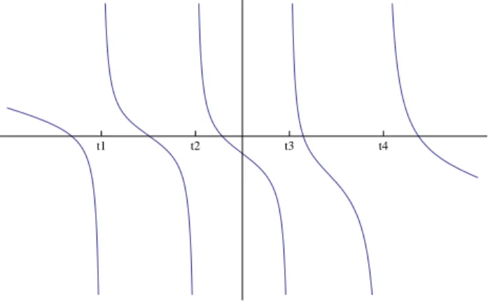
As a consequence of Lemma 4.1.1 we have that any rationalR-function of negative type is an (N + 1)-to-1 mapping with respect to λ on _R. The general shape of any rationalR-function of negative type is shown in Figure 4.1.

t1 t2 t3 t4

Figure 4.1. An example of S when N = 4.

4.2. Exactness and Ergodicity

Recall from Section 2.1 that a non-singular system (X,B, m, T) isergodic ifA∈ B is T-invariant implies m(A) = 0 or m(Ac_{) = 0. Furthermore, we say} _T _{is exact if}

A∈ B such that

(4.2.1) T−n(Tn(A)) =A for all n >0,

(44)

Recall that a consequence of Theorem 3.4.3 says that the restriction of a rational

R-function of positive type, F(x) = x +β +PN

k=1

pk

tk−x, where β, tk, pk ∈ R and

pk>0, is exact if β = 0. Otherwise,F is totally dissipative and nonergodic. We will appeal to this result while proving all rationalR-functions of negative type are exact, which in contrast to Aaronson’s result places no restriction on the constant, β. The following theorem is the main result of this section.

Theorem 4.2.1. Let S be a rational R-function of negative type. That is,

S(x) = −x−β− N

X

k=1

pk

tk−x

,

where tk, pk ∈ R and pk > 0. Then S is exact and ergodic with respect to Lebesgue measure.

Before proving Theorem 4.2.1 we note the following lemma on exactness of a transformation and its iterates

Lemma 4.2.2. If (X,B, m, T) is a nonsingular system such that T2 is exact with

respect to m, then T is exact with respect to m.

Proof. If A∈ B is a set for T as in (4.2.1), then T−2nT2n(A) =A for all n >0.

Thus, (T2)−n(T2)nA=A, soAalso has the property in (4.2.1) forT2. In other words we have

{A:T−nTnA=A, for all n >0} ⊆ {B : (T2)−n(T2)nB =B, for all n >0}.

T2 is exact, so all B as above have the property that m(B) = 0 or m(Bc) = 0. Therefore, the set A is such that m(A) = 0 orm(Ac_{) = 0, and} _T _{is exact.}

(45)

Proposition 4.2.3. Let S be a rational R-function of negative type. That is, S(x) = −x − β − PN

k=1

pk

tk−x, where β, tk, pk ∈ R and pk > 0. Then, S

2 _{is the}

restriction of a rational R-function of positive type, and S2 _{has form}

(4.2.2) S2(x) =x+

N2₊₂_N

X

k=1

ρk

τk−x

,

where τk, ρi ∈R, ρk >0.

The proof of Proposition 4.2.3 will require the following formula for partial fraction decomposition. Given two polynomials P(x) and Q(x) such that deg(P) < n and

Q(x) = (x−α1)· · ·(x−αn) where the αi are distinct, we have

(4.2.3) P(x)

Q(x) = n

X

i=1

P(αi)

Q0₍_α

i) 1 (x−αi)

.

Proof of Proposition 4.2.3. Suppose S is a rational R-function of negative

type as in the proposition. LetS2 _{be the second iterate of} _S_{. We have,}

(4.2.4) S2(x) = x+ N

X

k=1

pk

tk−x −

N

X

k=1

pk

tk−S(x)

,

where tk, pk ∈ R and pk > 0. The first two terms of (4.2.4) look like pieces from a rational R-function of positive type and are in the correct form. Considering the third term in (4.2.4) we will show that for a fixedk

(4.2.5) −pk

tk−S(x) =

N+1

X

j=1

ak,j

rk,j−x

,

where rk,j, ak,j ∈R and ak,j >0.

First, we write out the denominator of the left-hand-side of (4.2.5) and obtain

tk−S(x) = tk+x+β+ N

X

i=1

pi

ti−x

= (tk+x+β)

QN

i=1(ti−x) +

PN

i=1pi

Q

j6=i(tj−x)

QN

i=1(ti−x)

.

(46)

From Lemma 4.1.1 we have tk−S(x) = 0 has N + 1 distinct real solutions. That is,

S−1(tk) ={r(k,1), ..., r(k,N+1)}. Thus, (4.2.6) becomes

(4.2.7) −

QN+1

i=1 (rk,i−x)

QN

i=1(ti−x)

.

The negative in the numerator of (4.2.7) comes from the fact that ifN is even, then sign(xN+1_{) = +1, and if} _N _{is odd, then sign(}_xN+1_{) =} _{−1. Therefore, the entire}

fraction on the left-hand-side of (4.2.5) can be written

(4.2.8) −pk

tk−S(x) = pk

QN

i=1(ti −x)

QN+1

i=1 (rk,i−x)

= −pk

QN

i=1(x−ti)

QN+1

i=1 (x−rk,i)

.

Now, to use (4.2.3) we let

(4.2.9) P(x)

Q(x) = −pk

QN

i=1(x−ti)

QN+1

i=1 (x−rk,i)

,

and note that Q0(rk,j) =

QN+1

i6=j (rk,j−rk,i). Therefore,

P(x)

Q(x) = N+1

X

j=1

P(rk,j)

Q0₍_r_k,j) ·

1 (x−rk,j)

= N+1

X

j=1

−pk

QN

i=1(rk,j−ti)

Q

i6=j(rk,j−rk,i)

· −1 (rk,j−x)

= N+1

X

j=1

ak,j

rk,j−x

,

(4.2.10)

whereak,j = pk

QN

i=1(rk,j−ti) Q

i6=j(rk,j−rk,i). Finally, we will show thatak,j >0 for eachj = 1, ..., N+1.

We do this by considering the sign of the numerator and denominator separately. First, we consider the denominator of ak,j. We assume {r(k,1), ..., r(k,N+1)} are in

ascending order, so

(47)

Therefore, in the denominator of ak,j we have

(4.2.12) Y

i6=j

(rk,j−rk,i) = j−1

Y

i=1

(rk,j−rk,i)

| {z }

+

· N+1

Y

i=j+1

(rk,j−rk,i)

| {z }

(−1)N−j+1 .

Now, we consider the the numerator of ak,j. We know pk > 0. We also know there is exactly one rk,j in each atom of the partition in Lemma 4.1.1. That is,

rk,1 ∈(−∞, t1), rk,N+1 ∈ (tN,∞), and rk,j ∈(tj−1, tj) for j = 2, ...N. Thus, we have the following three cases:

(1) j > i =⇒ (rk,j−ti)>0, (2) j =i =⇒ (rk,j−ti)<0, and (3) j < i =⇒ (rk,j−ti)<0.

Therefore, we can count the number of sign changes coming from (1), (2), and (3) in the numerator of ak,j and obtain

(4.2.13)

N

Y

i=1

(rk,j−ti) = j−1

Y

i=1

(rk,j−ti)

| {z }

+

·(rk,j−tj)

| {z }

−1

· N

Y

i=j+1

(rk,j−ti)

| {z }

(−1)N−j

.

Thus, sign(ak,j) =

(−1)(N−j+1)

(−1)(N−j+1) which is positive. We have shown

S2(x) = x+ N

X

k=1

pk

tk−x + N X k=1 N+1 X j=1 ak,j

rk,j−x

= x+ N2₊₂_N

X

k=1

ρk

τk−x

,

(4.2.14)

where τk, ρk ∈Rand ρk>0.

Note that Proposition 4.2.3 shows that if S is a rational R-function of negative type, thenS2 _{is a rational} _R_{-function of positive type with constant term 0. We are}

(48)

Proof of Theorem 4.2.1. Let S be a rational R-function of negative type as

in the theorem. That is, S(x) = −x−β−PN

k=1

pk

tk−x whereβ, tk, pk ∈Rand pk >0.

Let S2 _{the second iterate of} _S_{. By Proposition 4.2.3 we have that} _S2 _{is a rational}

R-function of positive type and can be written

(4.2.15) S2(x) =x+

N2₊₂_N

X

k=1

ρk

τk−x

,

where τk, ρk ∈ R and ρk > 0. The constant term in S2 is 0, so we may appeal to Theorem 3.4.3 to obtain S2 is exact. Therefore, S is exact, by Lemma 4.2.2. Finally,

by Lemma 2.1.4 S is also ergodic.

4.3. Conservativity

Recall from Section 2.1 that a nonsingular system (X,B, m, T) is conservative if there does not exist a wandering set of positive measure. In other words, for allA∈ B with m(A)>0, there exists k >0 such that

(4.3.1) m(T−kA∩A)>0.

Again we consider rational R-functions of negative type, so

S(x) = −x−β− N

X

k=1

pk

tk−x

,

where β, tk, pk ∈R and pk>0.

Let ω1, .., ωN+1 denote the fixed points of S in ascending order. For the rest of

this chapter it is convenient to conjugateS so that ω1 = 0. That is, S(0) = 0 and all

other fixed points are positive. Let

φ(x) = x−ω1 and φ−1(x) = x+ω1.

(49)

˜

S(x) =−x−2ω1−β−

N

X

k=1

pk (tk−ω1)−x

.

We note that ˜S(0) = (φ ◦S ◦φ−1)(0) = (φ ◦S)(ω1) = φ(ω1) = 0. Also, if the

poles of S are {t1, ..., tN} in ascending order, then the poles of ˜S are tk −w1 for

k = 1, ..., N in ascending order. The smallest pole of ˜S is t1 −w1 which is greater

than 0. Furthermore, φ:S →S˜ is an isomorphism (as in Definition 2.1.9), soS and ˜

S have the same measure theoretic properties. Thus, without loss of generality we may assume that ω1 = 0 is the smallest fixed point of S, and all other fixed points,

{ωi}N_i₌₂+1, as well as all the poles, {ti}N

i=1, are positive. For the rest of this chapter we

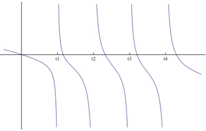
assume S has the general shape in Figure 4.2.

t1 t2 t3 t4

Figure 4.2. An example of conjugated S when N = 4.

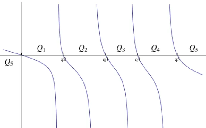
Let q1, ..., qN+1 denote the roots of S. Note that q1 = ω1 = 0. We define a

partition Q = {Q1, ..., QN+1} of R to be the intervals between the roots. That is,

Qi = [qi, qi+1) for i= 1, ..., N and QN+1 = (∞, q1)∪[qN+1,∞). The general shape of

S along with the partition Qare depicted in Figure 4.3.

Remark 4.3.1. Using a process similar to that in Lemma 4.1.1 we knowS maps

(50)

Q1 Q2 Q3 Q4 Q5

Q5 q2 q3 q4 q5

Figure 4.3. An example of theQ partition for S whenN = 4.

The above remark motivates the following notation. We letψi denote the inverse of S restricted toQi. That is

(4.3.2) ψi =S−1|Qi,

so ψi :R→Qi is one-to-one and onto for i= 1, ..., N + 1. We denote the refinement

Qi1 ∩S

−1_Q

i2 ∩...∩S

−(n−1)_Q

in by Qi1...in, and let

(4.3.3) ψi1...in =S −1_|

Qi₁...in, so ψi1...in =ψi1...in−1 ◦ψin.

Note that ψi1...in : R → Qi1...in is one-to-one and onto. We define one more piece of

notation and let

(4.3.4) ψi[k]=ψi◦ψi◦...◦ψi

| {z }

k−times

.

Proposition 4.3.2. The set A = SNi=1Qi = [q1, qN+1] is a sweep-out-set for S.

That is, S

n≥0S

−n_A₌

R mod λ.

Before we prove Proposition 4.3.2 we need the following lemma.

Lemma 4.3.3. Let {xk}∞k=0 be a sequence of positive numbers. If c is a positive

constant and x2

k+1 ≥x2k+c, then xk >

pc

2 ·

√

5079.pdf

Entropy of Transformations that Preserve an Infinite Measure

Abstract

Acknowledgments

Table of Contents

List of Figures

INTRODUCTION

BACKGROUND

R-FUNCTIONS

RATIONAL

R-FUNCTIONS OF NEGATIVE TYPE