GEOVISUALIZATION OF MOUNTAIN HYDROCLIMATIC VARIABILITY: LINKAGES BETWEEN ATMOSPHERIC CIRCULATION AND THE SPATIAL PATTERN OF
PRECIPITATION
Johnathan W. Sugg
A dissertation submitted to the faculty at the University of North Carolina at Chapel Hill in partial fulfillment of the requirements for the degree of Doctor of Philosophy in the Department
of Geography.
Chapel Hill 2017
Approved by: Charles E. Konrad II Erika K. Wise
Diego A. Riveros-Iregui Ryan P. Boyles
iii ABSTRACT
Johnathan W. Sugg: Geovisualization of Mountain Hydroclimatic Variability: Linkages Between Atmospheric Circulation and the Spatial Pattern of Precipitation
(Under the direction of Charles E. Konrad II)
The hydroclimatology of mountain regions is important for the world’s water resources, yet is poorly understood in the context of climate variability and change. Observations indicate that drought and heavy precipitation have increased throughout the mid-latitudes during the last century, and future projections show a continuation of these trends. Despite these predictions, our understanding of the physical processes and associated spatial patterns of precipitation in mountains is lacking. In order to make better predictions of hydroclimatic change in mountain regions, research is first needed to understand the relationship between atmospheric circulation and precipitation. The purpose of this dissertation is to examine this relationship in the southern Appalachian Mountains of the southeastern United States, a mid-latitude mountain region that exhibits much hydroclimatic variability. I use both established and innovative geovisualization techniques to reveal how topographic features mediate the relationship between large scale circulation and precipitation characteristics. First, I compare several types of statistical clustering algorithms to identify hydroclimatic regions based on commonalities in the type and frequency of summer rainfall. Second, a self-organizing map is used to classify and visualize patterns of synoptic-scale circulation variability. The identified patterns are then linked with daily
iv
new graphical representation for displaying simple spatial statistics of the precipitation
v
vi
ACKNOWLEDGEMENTS
I wish to thank my dissertation chair and committee members. In particular, I give a deep thank you to my chair and adviser – Chip Konrad – for years of careful mentorship. His close guidance in climatology and attention to detail in my writing allowed me to develop the toolkit that I needed to undertake this project. I am grateful to Ryan Boyles, who provided expertise on the use of precipitation datasets and precipitation estimation in mountain regions. I thank Tom Rickenbach, who provided a valuable perspective on precipitation processes across the
southeastern United States and challenged me to consider the contribution of my research. Much appreciation goes to Diego Riveros-Iregui for his insight on the ecohydrologic implications of precipitation in mountains and research in general. I also thank Erika Wise, who provided much expertise on the use of self-organizing maps and encouraged me to use the technique in my research.
I wish to thank the Southeastern Regional Climate Center and the Department of Geography at UNC-Chapel Hill for research, travel, and assistantship funding support as I worked on this dissertation. The Suzanne Levy Summer Research Fellowship at UNC-Chapel Hill also funded this research.
vii
viii
TABLE OF CONTENTS
LIST OF TABLES ... xi
LIST OF FIGURES ... xii
LIST OF ABBREVIATIONS ... xiv
CHAPTER 1: INTRODUCTION ... 1
Introduction and Research Context ... 1
Research Objectives ... 2
Theoretical Framework ... 4
[Cartography]3 in Geographic Research ... 4
Dissertation Outline ... 6
CHAPTER 2: DISENTANGLING THE SPATIOTEMPORAL COMPLEXITY OF OROGRAPHIC PRECIPITATION PATTERNS IN THE SOUTHERN APPALACHIAN MOUNTAINS... 8
Introduction ... 8
Background ... 10
Study Area ... 11
Precipitation Data... 13
Classification of Precipitation Events ... 14
Visualization of Precipitation Events... 18
Cluster Analysis of Precipitation Events ... 22
ix
Visualization of Hydroclimatic Regions ... 31
Conclusions ... 38
CHAPTER 3: RELATING WARM SEASON HYDROCLIMATIC VARIABILITY IN THE SOUTHERN APPALACHIANS TO SYNOPTIC WEATHER PATTERNS USING SELF-ORGANIZING MAPS ... 40
Introduction ... 40
Synoptic Scale Circulation Controls on Precipitation in Mountains ... 41
Spatiotemporal Patterns of Precipitation ... 42
Study Area – Southern Appalachian Mountains ... 44
Data ... 47
Implementation of the Self-Organizing Map (SOM)... 48
Classification of the Synoptic Scale Circulation ... 50
The Hydroclimate of the SAM and its Relationship with Circulation Patterns ... 54
Summary and Conclusion ... 63
CHAPTER 4: IMPROVING THE GRAPHICAL REPRESENTATION OF COMPLEX CLIMATE PATTERNS WITH SELF-ORGANIZING MAPS ... 67
Introduction ... 67
Implementation of the SOM in Geographic Information Science ... 69
Methods... 71
Study Area – Southern Appalachian Mountains ... 71
Implementation of the SOM in this research ... 73
Case Study ... 78
Circulation Patterns Identified in the SOM ... 79
Computation and Visualization of Spatial Statistics in SOM-Space ... 80
x
Standard Distance ... 83
Discussion and Conclusions ... 85
CHAPTER 5: SUMMARY... 90
Research Contribution ... 93
Direction of Future Research ... 96
xi
LIST OF TABLES
xii
LIST OF FIGURES
Figure 1.1: Cartography cubed model ... 6
Figure 2.1: Study are map of the southern Appalachian Mountains... 13
Figure 2.2: Average summer rainfall and frequency of days with rainfall. ... 17
Figure 2.3: Average frequency of different precipitation events ... 18
Figure 2.4: Google Earth scene of topographic transect ... 20
Figure 2.5: Geovisualization of average frequency of different precipitation events ... 21
Figure 2.6: Standardized frequency of different precipitation events... 25
Figure 2.7: Geovisualization of standardized frequency of different precipitation events ... 27
Figure 2.8: Visual cluster analysis evaluation. ... 29
Figure 2.9: Geovisualizations of clustering results ... 33
Figure 2.10: PAM 5 clustering results ... 34
Figure 2.11: Scatterplot matrices of different precipitation events ... 35
Figure 2.12: Barplots of regional hydroclimatic character ... 37
Figure 3.1: Study area map of the southern Appalachian Mountains ... 46
Figure 3.2: Study domain map and quadrangle ... 48
Figure 3.3: Self-organizing map of 500 mb geopotential height ... 53
Figure 3.4: Composited mean sea level pressure in the self-organizing map ... 54
Figure 3.5: Frequency of different precipitation events over the study period ... 57
Figure 3.6: Days with no rainfall in the self-organizing map ... 58
Figure 3.7: Days with very light rainfall in the self-organizing map ... 59
Figure 3.8: Days with light rainfall in the self-organizing map ... 60
xiii
Figure 3.10: Days with heavy rainfall in the self-organizing map ... 62
Figure 3.11: Summary results with wind direction in the self-organizing map... 62
Figure 4.1: Elevation, hydroclimatic regions, and frequency of rainfall ... 73
Figure 4.2: Study domain map and quadrangle ... 74
Figure 4.3: Self-organizing map of 500 mb geopotential height ... 75
Figure 4.4: Composite mean sea level pressure and wind direction in the self-organizing map .. 76
Figure 4.5: Frequency of precipitation across the hydroclimatic regions in each node ... 77
Figure 4.6: Precipitation centroid locations in the self-organizing map ... 81
xiv
LIST OF ABBREVIATIONS
CLARA Clustering large applications CV Climate visualization
DEM Digital elevation model
ECMWF European centre for medium range weather forecasting GPH Geopotential height
MPE Multisensor precipitation estimate MSLP Mean sea level pressure
NASH North Atlantic subtropical high PAM Partitioning around medoids
PRISM Parameter regression on independent slopes model SAM Southern Appalachian Mountains
1
CHAPTER 1: INTRODUCTION
Introduction and Research Context
The hydroclimatology of mountain regions is important for the world’s water resources, yet is poorly understood in the context of climate variability and change. Observations indicate that drought and heavy precipitation have increased throughout the mid-latitudes during the last century (Hartmann et al. 2013), and future projections show a continuation of these trends (Christensen et al. 2013). Despite these predictions, our understanding of the physical processes and associated spatial patterns of precipitation in mountains is still lacking (Barry 2008).
Synoptic circulation patterns and their interaction with prominent topographic features show a considerable influence on the spatial variability of precipitation. In order to make better
predictions of hydrologic change in mountain regions, research is first needed to understand the effect of atmospheric circulation on precipitation patterns (de Jong et al. 2009; Kelly et al. 2012).
This dissertation examines the relationships between hydroclimatic variability and synoptic-scale circulation in the southern Appalachian Mountains (SAM), located in the
southeastern U.S. (SEUS). Within this region, drought and heavy precipitation have increased in recent decades (Labosier and Quiring 2013). In mountain regions, topography both increases and decreases precipitation rates across small areas, subsequently increasing the likelihood of
extreme hydroclimatic events (Diaz et al. 2003; Fuhrmann et al. 2008).
2
population centers (Mote et al. 2005). In the SEUS, headwater catchments along the SAM supply freshwater to several of the most rapidly growing metropolitan areas, including Atlanta, Georgia, Charlotte, North Carolina, and Knoxville, Tennessee (Kramer and Eisen-Hecht 2002; Ruhl 2005). Additionally, heavy rainfall in mountain regions increases stormflow runoff and flooding, especially in portions of the SAM, where surface mining (e.g. strip mining) and reclamation result in deforestation and soil compaction (Negley and Eshleman 2006). The hydroclimate also regulates valuable ecosystem services. The SAM is home to an International Biosphere Reserve and an United Nations Educational, Scientific, and Cultural Organization World Heritage Site, and their respective ecosystems house a variety of biologically diverse and endemic species. Endangered, Red spruce-Fraser fir species in mountain cloud forests (Reinhardt and Smith 2008) and Plethodon salamanders (Caruso et al. 2014) are two examples of species that are particularly vulnerable to future changes in the hydroclimate.
Research Objectives
This dissertation examines the relationships between mountain hydroclimatic variability and synoptic-scale circulation in the SAM. The objective of this research is to use both
established and innovative climate visualization techniques to reveal how topographic features mediate the relationship between large scale circulation and precipitation characteristics at the surface, effectively characterizing the hydroclimatic variability. Climate visualization refers to the transdisciplinary field of research and science communication that seeks to develop
3
1. How does daily precipitation vary through space and time in the SAM? What is the spatial pattern of different types of precipitation events? Which physiographic regions across the SAM are most prone to hydroclimatic extremes?
2. What synoptic patterns are tied to different precipitation events in the SAM during the warm season? Among the identified patterns, what is the spatial distribution of precipitation events across the different physiographic regions of the SAM?
3. To what extent do changes in the synoptic-scale circulation pattern influence the distribution of different types of precipitation events across the different
physiographic regions?
Three working hypotheses drive this research:
1. Shifts in the lower tropospheric circulation lead to pronounced and measurable changes in the precipitation frequencies and amounts across some regions of the SAM. These shifts influence the propagation and organization of rainfall around topographic features.
2. Broad scale regions of high elevation promote greater frequencies of light
precipitation events at the daily scale. This precipitation regime leads to extended periods of wetness and may play a role to inhibit the development of drought. This persistent pattern of light precipitation is present, to varying degrees, no matter what synoptic circulation pattern is present.
4
moisture into the region and promotes unstable conditions in the column (e.g. presence or approach of a middle tropospheric trough).
Theoretical Framework
[Cartography]3 in Geographic Research
This dissertation utilizes geospatial modeling and geovisual analytics (Virrantaus et al. 2009). The two research areas are readily integrated with climatology in a theoretical framework of cartographic communication and visualization. This framework allows the researcher to enhance geographic communication on issues such as climate variability and change by
leveraging new visualization techniques for knowledge discovery and data mining. It is situated within the [Cartography]3 model of map use, first developed by DiBiase (1990) and then
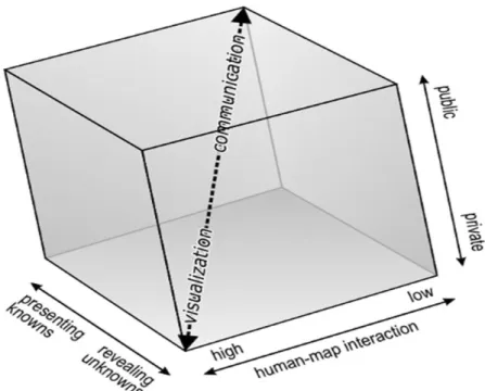
updated by MacEachren (1994) (Figure 1.1). The model distinguishes between two intended map uses in geographic research, which are laid out along an axis that connects opposite vertices of a transparent cube. On one end, visualization is the intended form of map use. Communication is the intended form of map use on the opposite end.
The characteristics associated with both extremes of the model are revealed along the three dimensions of the cube. The first dimension of the cube determines the purpose of the map, which can be used to present knowns or reveal unknowns within the data. The second dimension describes the degree of human-map interaction, which can be high or low. The third dimension of the cube designates whether the map use is conducted among a public or private audience.
5
required to understand the patterns that are represented. Interactivity between the map and the user is low, since the map cannot respond to inputs from the user.
On the opposite end of the cube, visualization is used to reveal unknown patterns and relationships about geographic phenomena. It provides a powerful tool to the researcher because it has the capability to reveal patterns within a dataset in an exploratory environment. The
visualization process is therefore typically carried out in private, among researchers, who may be interested in developing hypotheses through the data exploration process. The degree of human-map interaction is high due to the ability of the researcher to manipulate the attributes and display of geographic variables within the visualization.
The art and science of cartography have changed very little, yet the technology has changed drastically. Whereas the communication model of map use is primarily driven by the fundamental design principles of cartography (i.e. the art and science), the visualization model is driven by increases in computational power (i.e. the technology) over the last several decades. Improvements in computing have also increased the ease with which scientists are able to manipulate large multidimensional datasets into useful visualizations and models (MacEachren and Kraak 2001).
Climatology is a useful domain for the application of this theoretical framework because it contains many characteristic challenges that are common in geographic research. Climate science is generating very large and complex spatiotemporal datasets for analytical work (Nocke et al. 2004). These data contain multiple types of uncertainty, are generated at multiple scales, and include temporal attributes. These characteristics are particularly challenging for the
6
climate research and other areas in science (Neset et al. 2009). Researchers across the geographic discipline, not just cartographers, should take care to develop techniques that benefit from the capabilities of visualization yet retain the ability to communicate about geographic phenomena in large, complex datasets.
Figure 1.1: Cartography cubed model of map use (Source: MacEachren 1994).
Dissertation Outline
7
Chapter 3 is titled “Relating Warm Season Hydroclimatic Variability in the Southern Appalachians to Synoptic Weather Patterns Using Self-organizing Maps.” It relates the
hydroclimatic patterns across the SAM to atmospheric circulation patterns in a visual way that is accessible to a variety of audiences. This chapter also provides an overview of the
self-organizing map technique as a spatially organized visualization tool that is suitable for classifying the large scale atmospheric circulation.
Chapter 4 improves the interpretability of the self-organizing map output by calculating spatial statistics to determine the circulation patterns that are most and least tied to the different types of precipitation events in each region of the SAM. Weighted mean center and standard distance are computed in the array of the self-organizing map and displayed cartographically in a new graphical representation to identify, distinguish, and rank precipitation characteristics across the topographic regions in the SAM.
8
CHAPTER 2: DISENTANGLING THE SPATIOTEMPORAL COMPLEXITY OF OROGRAPHIC PRECIPITATION PATTERNS IN THE SOUTHERN APPALACHIAN
MOUNTAINS
Introduction
Climate visualization (CV) is an emerging geovisualization technique for identifying and interpreting climate patterns from large geospatial datasets. Improvements in computing have increased the ease with which these datasets can be translated into a variety of useful maps, plots, and 3+ dimensional models. Hypothetically, these products facilitate easier knowledge exchange between researchers and policymakers (Hulme 2014). However, many challenges continue to limit the interpretation and communication of research that is generated using these datasets (MacEachren and Kraak 2001; Virrantaus et al. 2009).
While much geographic research on big data has investigated the emergent challenge of data size, little research has focused on the challenge of complexity (Miller and Goodchild 2015). Complexity has been defined in numerous ways over the last several decades (Fairbairn 2006). In cartographic research, it is commonly understood as the degree of visual
interconnectedness of components or patterns in a structure (MacEachren 1982). Complexity may also be extended to describe the physical features of earth systems since there are multiple interactions between many different components (Rind 1999). For example, orographic
9
Cartographers have long been interested in simplifying complexity both in a visual map-sense and intellectually by increasing the ease with which features are understood (Fairbairn 2006). However, the growth in attributes and dimensions of geospatial data means that this challenge is no longer held strictly within the domain of cartographic research. For example, the higher resolution of interpolated raster data shows increased surface roughness, patchiness, or interdigitation of climatological and ecological features. Researchers across the geographic discipline are thus presented with the challenge of simplifying complex patterns into interpretable components using effective visualizations.
CV is suitable for unraveling the complexity in multidimensional data for several
reasons. First, it is interactive. The user may take a grand tour of the data space and therefore has the ability to perform a guided search or exercise manual control in order to visualize
relationships in a 3D environment (Macedo et al. 2000). CV is also a useful aid in the application and interpretation of spatial statistics. It can be utilized for the selection, parameterization, and comparison of different statistical cluster analyses, in addition to the interpretation of the final clusters themselves (Nocke et al. 2004). Finally, it exploits the capabilities of human perception. For example, effective use of color in meteorological visualizations is shown to improve the simplicity and speed with which the user uncovers important features or anomalies in climate fields (Stauffer et al. 2015).
10
examine simple geovisualizations that are created in Google Earth to explore the spatial pattern of daily precipitation events over a 3D virtual globe. The daily precipitation fields are used as input to a statistical cluster analysis in order to identify hydroclimatic zones across the terrain. A geovisualization of these zones (i.e. clusters) is then used to effectively interpret and
communicate to a general audience the significance of the various hydroclimatic regions. Background
The hydroclimatology of mountain regions is complex for several reasons. First, the spatial patterns of precipitation in mountain regions are not well documented or understood, primarily because they are difficult to observe (Barry 2008). Meteorological instrumentation is typically confined to valley locations, which limits observations from higher terrain in remote areas. Regression-based studies (Basist et al. 1994; Hevesi et al. 1992; Konrad 1996) have identified relationships between these spatial patterns of precipitation and topographic attributes, but they are subject to the limitation of station locations.
Second, the spatial pattern of precipitation and its distribution are highly variable across mountain catchments due to topographic complexity. Topographic complexity is defined as any change to the land surface attributes, including the aspect, elevation, and slope, over a distance. Relationships exist between topographic complexity and precipitation rates over short distances that influence the likelihood of extreme events (Diaz et al. 2003; Fuhrmann et al. 2008). For example, prominent ridgelines, concave areas, and broad, high plateaus increase the frequency of precipitation events (Lin et al. 2001), while decreases in the frequency of precipitation events are found leeward of these topographic features.
11
different types or classes of daily precipitation events (e.g. from days with no precipitation to days with heavy precipitation) and display them cartographically. It is the occurrence or
frequency of these events on a daily basis that will aid the identification of areas across mountain catchments where hydroclimatic extremes such as drought or heavy rainfall are likely to develop. Representations of the complexity in the precipitation pattern would greatly benefit a wide range of audiences, and CV can provide an effective tool to communicate these representations.
Three brief examples of the benefits are provided: (1) CV assists in the provisioning and planning of ecosystem services by conservation managers, including the biodiversity of montane species whose ecological ranges depend upon the persistence of moist conditions at the surface. (2) It improves inputs to water availability in municipal water resource models because different types of precipitation events exhibit different types of hydrological responses across mountain catchments. For example, a light rainfall event during the leaf-on season is likely to produce a minimal hydrologic impact, as canopy interception minimizes the amount of precipitation throughfall to the soil (Vose et al. 2016). (3) CV aids in forecasting of precipitation in mountain regions and surrounding lowland areas because it helps to pinpoint regions where precipitation hazards, such as drought and flood-producing precipitation, are most likely to occur.
Study Area
12
from roughly 900 mm (35 in.) in various rain shadowed valleys to nearly 2500 mm (98 in.) (Kelly et al. 2012) on prominent ridgelines, which are directly exposed to moisture advection from the Atlantic Ocean and Gulf of Mexico (Konrad 1996).
Four physiographic regions make up the SAM. 1) The Cumberland and Allegheny Plateaus in the northwest portion of the SAM are generally above 500 m and are highly incised by dendritic stream networks. 2) The Valley and Ridge region lies further southeast and consists of generally long and relatively straight ridges with elevations ranging from 600 to 1000 m. On the southeast side of the province, some of the intervening river valleys are quite large and relatively flat in places. This region includes the New River and Tennessee Valleys. 3) The most prominent ridgelines and highest elevations (>2000 m) are located in the topographically
13
Figure 2.1: Elevation and distribution of topographic regions across the southern Appalachian Mountains.
Precipitation Data
This study utilizes fine-scaled raster precipitation estimates that offer the benefit of being continuous across space, as opposed to irregularly spaced point observations (i.e. rain gauges). These estimates are obtained from daily, gridded PRISM precipitation fields (Prism Climate Group 2015). They are provided at a 4x4 km resolution of grid cells over the U.S. at daily time steps. PRISM estimates are particularly suited to studies in mountainous terrain. The
14
characteristics that influence precipitation development. Since 2002, multi-sensor precipitation estimates (MPE) are incorporated into the PRISM geographically-weighted regression. This improves PRISM precipitation estimates because the MPE offer gauge-calibrated radar estimates of daily precipitation to refine the regression model. PRISM is therefore a hybrid estimate of both gauge-calibrated radar observations and station derived precipitation observations. When compared to MPE alone, which are limited by radar beam blockage in mountainous terrain (Wootten and Boyles 2014; Zhang et al. 2011), the daily PRISM estimate presents a more
accurate portrait of historical daily precipitation amounts. Daly et al. (2008) provide more details on this technique. Daily data were collected for this study from 2002-2014 for the months of June, July, and August. This daily time series is sufficiently long enough to identify reoccurring spatial patterns of precipitation that characterize the warm season hydroclimatology of the region.
Classification of Precipitation Events
15
event types: very light (0.25 – 2.54 mm), light (2.55 – 12.7 mm), moderate (12.8 – 38.1 mm), and heavy (≥ 38.1 mm).
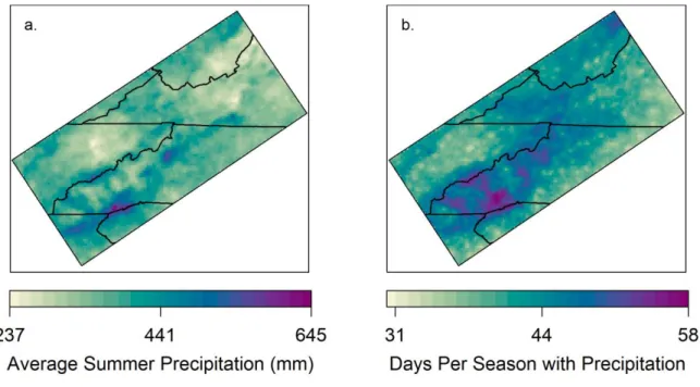
A comparison of the average summer season precipitation and the seasonal frequencies of precipitation are presented in Figure 2.2. There is much variability in the spatial pattern of
average summer precipitation. On a local scale, rain-shadowed valleys receive less precipitation than the adjacent ridges. The larger valleys (e.g. the French Broad, New, and Tennessee valleys) are the driest, receiving less than 254 mm (10 in.) of precipitation in places. These valleys are shielded from moisture advection in nearly every direction, making them the driest locations in the interior southeastern US. Higher precipitation amounts (>381 mm (15 in)) are found along the western slopes of the Allegheny Plateau, Cumberland Plateau, and Great Smoky Mountains, as these areas are exposed to moisture advection from the west and northwest. However, the most precipitation (>508 mm (20 in)) occurs in the Blue Ridge region, which is directly exposed to moisture advection from the south and southeast. This is especially the case along the southern Blue Ridge Escarpment in western North Carolina, which is the wettest region in the interior southeastern US. The town of Highlands, located at the top of the escarpment, in fact, holds a record for the greatest one-day precipitation event (537.21 mm (21.15 in)) in North Carolina (SCO-NC 2015). These patterns line up well with previously documented orographic
precipitation patterns in the SAM (Kelly et al. 2012; Konrad 1996).
16
a higher elevation. Precipitation occurs frequently at 45 – 50 days per season across areas of higher elevation (>1000 m) in southwestern North Carolina, northwestern North Carolina, the Cumberland Plateau in far southwestern Virginia, and the Allegheny Plateau in West Virginia. Precipitation is most frequent across the exposed ridgelines in western North Carolina, which includes the Great Smoky Mountains, Balsam and Black Mountain ranges, and the southern Blue Ridge Escarpment. There are more than 55 days with precipitation in these areas, which is more than half of the days during the summer season. This pattern also includes several of the narrow interior river valleys in southwestern North Carolina and indicates that portions of the SAM, including some areas with lower average summer precipitation, are frequently wetted over the course of the summer.
The spatial patterns of the return period for each precipitation event type are presented in Figure 2.3. Very light and light precipitation events occur most frequently. There are 18 – 20 days per season with very light precipitation events across the higher elevation regions of the SAM, with the frequencies greatest along the southern Blue Ridge Escarpment. In the Tennessee valley and Piedmont, very light precipitation occurs 10 days per season. Light precipitation occurs most frequently along the high elevation plateau in southwestern North Carolina, Blue Ridge Escarpment, exposed ridgelines of the Balsam and Black Mountain ranges, and the Allegheny Front. In these regions, it occurs more than 24 days per season. Light precipitation is least frequent in the Tennessee valley and Piedmont, occurring 14 days per season. Combined, very light and light precipitation characterize nearly 50% of the total precipitation events across the high elevations in the SAM during the summer season.
Moderate and heavy precipitation events occur least frequently across the SAM.
17
Smoky Mountains and the southern Blue Ridge Escarpment. Along the Allegheny Front and northern Blue Ridge Escarpment, moderate precipitation events occur 10 days per season. They occur least frequently in the rain-shadowed French Broad, Tennessee, and New River valleys, less than 6 days per season. Heavy precipitation events occur most frequently (2 – 3.5 times per season) along the Blue Ridge Escarpment and the adjacent Piedmont.
18
Figure 2.3: Comparison of the average number of days per season with (a.) very light, (b.) light, (c.) moderate, and (d.) heavy precipitation events.
Visualization of Precipitation Events
web-19
based virtual globe for simple visualizations of raster data, and scientists have increasingly used its capability to communicate research findings (Goodchild 2008; Yu and Gong 2012). Its interface offers the user an opportunity to engage and interact with the precipitation surface by manually panning and zooming over the virtual globe at a fine spatial resolution. The user can explore precipitation patterns across different topographic settings from any height or
perspective, and can utilize this capability as a mechanism for hypothesis generation (Butler 2006). For example, users can hypothesize how the distribution of precipitation events over different topographic regions is likely to influence the spatial pattern and composition of the resulting regions in a statistical cluster analysis.
There are cognitive limitations of the visualization of geospatial data in a 3d environment (Slocum et al. 2001). For example, much research has identified the use of oblique 3d views with overlaid raster data as problematic for map interpretation and reading (Elmqvist and Tsigas 2008). Occlusion limits the perspective of the user and is particularly challenging when the objective is to discern regional scale patterns. However, this application is interactive and it is used for exploratory visualization of precipitation patterns at local scales.
20
situated in the rain-shadowed French Broad River valley located further west, and has an average summer precipitation of 254 mm (10 in.) (Arguez et al. 2010).
Figure 2.4: Google Earth scene across a topographic transect from Asheville, North Carolina, in the valley bottom, to Mt. Mitchell, across the ridgeline in the background. Photographic imagery Copyright
2016. Image: Landsat. Data: SIO, NOAA, U.S. Navy, NGA, GEBCO.
To enhance the interpretability of precipitation patterns, a visualization of the spatial pattern of the return period for each precipitation event type is presented in Figure 2.5. Precipitation events occur most frequently for all event types along the exposed ridgeline and higher elevations in the background. There are, however, some variations in the altitudinal changes across each type. There is only a slight decrease in the frequencies of very light
precipitation from the ridge top (18 events per season) down to the valley bottom (16 events per season). Light, moderate, and heavy precipitation events show much greater changes in
21
ridge tops (>26 days per season) and decrease to 15 days per season in the valley bottom. Moderate precipitation events occur 10 days per season across the exposed southeastern ridge tops and less than 6 days per season in the river valley. Heavy precipitation events occur 2 days per season across the highest ridge tops, and occur less than one day per season in the valley bottom.
Figure 2.5: Geovisualization depicting the average number of days per season with (a.) very light, (b.) light, (c.) moderate, and (d.) heavy precipitation events across the topographic transect. Photographic
22 Cluster Analysis of Precipitation Events
In this study, cluster analysis is used to recast the complex spatial structure of
hydroclimatic patterns into readily identifiable and interpretable regions that exhibit similarities in precipitation. Cluster analysis is a common technique used in climatological research to arrange data into homogenous groups around a centroid, or measure of central tendency (Fovell 1997). It maximizes the difference between clusters and minimizes the difference within clusters by calculating a minimum distance measurement between the centroid and each observation in the data space (Kalkstein et al. 1987; Konrad 1997). Depending on the type of algorithm that is chosen, each grid cell is examined to determine its Euclidean distance from other cells. As grid cells are continually assigned to centroids that share similar characteristics, this process is repeated until the finalized clusters are achieved. At this stage, its output is rendered as a static plot in two dimensions, and traditionally serves as a useful tool for both exploration and interpretation of the resulting regions (Stooksbury and Michaels 1991).
There are several clustering algorithms suitable for determining groups in climate data. We compare three standard partitioning algorithms using programs for K-means, partitioning around medoids (PAM), and clustering large applications (CLARA). The specific parameters of each algorithm are discussed in detail in Maechler et al. (2013), and based on the work of Kaufman and Rousseeuw (1990). Sample routines for each application are carried out with five, six, and seven number of clusters to assess the sensitivity of the resulting hydroclimatic regions to variations in each algorithm.
In order to carry out the analysis, the frequency of precipitation event types are
23
observed over all grid cells. For each grid cell, we take the observed frequency of the
precipitation event type, subtract the mean frequency, and divide by the standard deviation. This step produces four raster surfaces in which grid cell values are z-scores of each precipitation event type. The standardized frequency of different precipitation events thus provides a
dimensionless measure of their occurrence across the region relative to the mean. This step also insures that each cluster variable is weighted equally before it is used as an input to the cluster analysis.
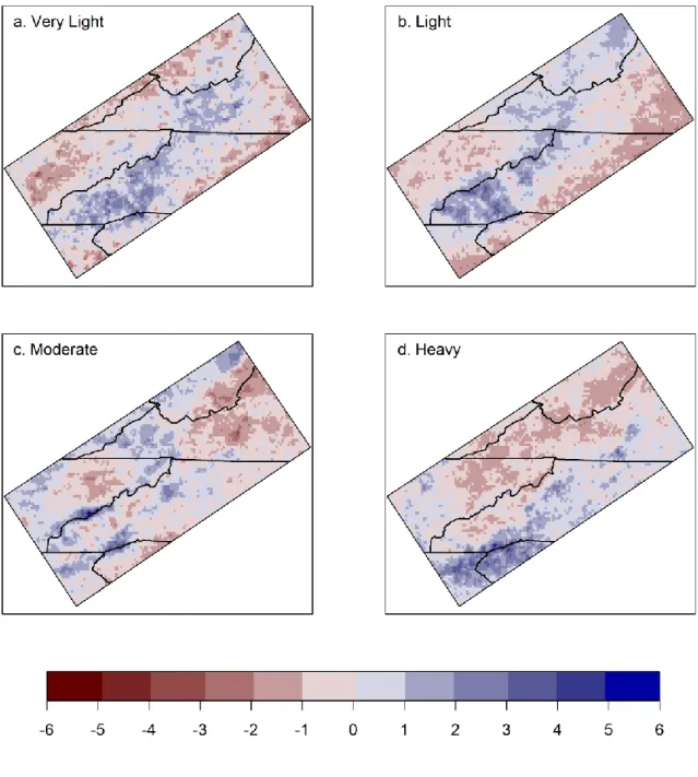
Figure 2.6 presents the standardized frequency of the precipitation event types. We use a red-to-blue diverging color palette to emphasize the relative difference in the return period of precipitation event types above or below the mean. The z-score patterns for each precipitation type enables us to hypothesize which topographic regions will share similar precipitation characteristics. High z-scores in blue emphasize regions where precipitation is most frequent compared to the mean. Low z-scores in red emphasize regions where precipitation is least frequent compared to the mean. Many of these patterns have a connection with the terrain in Figure 2.1. For example, very light and light precipitation events are widespread among the various topographic regions across the SAM. Days with very light precipitation are most
frequent in high elevation regions, which include the Blue Ridge Escarpment, Balsam and Black Mountain ranges. However, they are also frequent in various valleys, including the New River and French Broad valleys. This pattern shares much in common to the days with light
24
within the interior of the SAM as a contiguous hydroclimatic region, which features higher frequencies of very light and light precipitation events.
25
Figure 2.6: Standardized frequency of (a.) very light, (b.) light, (c.) moderate, and (d.) heavy precipitation events.
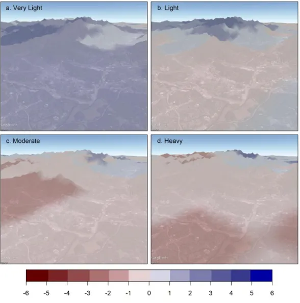
CV is employed to examine the standardized frequencies in relationship with the terrain in Figure 2.7. Days with very light precipitation events are frequent across much of the
26
27
Figure 2.7: Geovisualization depicting the standardized frequency of (a.) very light, (b.) light, (c.) moderate, and (d.) heavy precipitation events across the topographic transect. Photographic imagery
Copyright 2016. Image: Landsat. Data: SIO, NOAA, U.S. Navy, NGA, GEBCO.
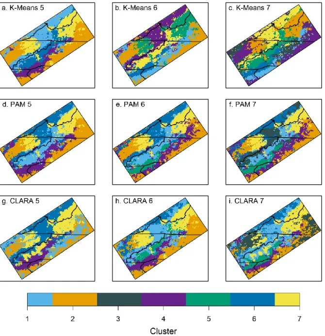
The results from K-Means, PAM, and CLARA clustering algorithms are presented in Figure 2.8. Increasing the number of clusters in each technique adds spatial complexity to the resulting regions. For example, each of the clustering procedures with seven regions introduces unnecessary interdigitation between grid cells with opposing cluster membership, increases noise or patchiness, and simultaneously reduces the overall interpretability of the hydroclimatic
28
29
Figure 2.8: Performance comparison of clustering results with five (left column), six (center column), and seven (right column) number of clusters. Clustering results from K-Means (upper row), PAM (center
row), and CLARA (lower row) clustering algorithms are compared. A single legend is used for all combinations, however certain cluster numbers (e.g. 3, 5) will not be used in each column.
Cluster Validation
30
used to measure the extent to which the grid cells are placed in the same cluster as the nearest neighbor grid cells. Connectivity is a characteristic that improves the interpretability of the resulting regions. Lower values indicate a higher degree of connectivity in which large groups of grid cells are located in similar topographic environments. Clustering algorithms for K-Means 5 and PAM 5 exhibit the highest hydroclimatic regional connectivity, while PAM 7 and CLARA 7 exhibit the least connectivity.
Second, the Dunn index (Dunn 1974) and the silhouette width (Rousseeuw 1987) are used to combine statistical measures of cluster compactness and separation into a single index. Compactness is a characteristic of cluster homogeneity and it is calculated based on the intra-cluster variance of grid cell values. Separation is determined by measuring the distance between cluster centroids. Compactness increases along with the number of clusters while separation decreases as the regions become interdigitated (Brock et al. 2008). The Dunn index measures this relationship as a ratio between zero and ∞, with maximum values indicating good cluster
performance.
In Table 2.1, PAM 5 and PAM 7 exhibit the lowest Dunn index value, indicating an uneven relationship between the degree of regional compactness and separation. Both clustering algorithms result in hydroclimatic regions with elongated and sinuous spatial patterns which are difficult to interpret in Figure 2.8. CLARA 5 and K-Means 5 exhibit the greatest Dunn index values, indicating that hydroclimatic regions have compact cluster shapes and relatively even distances between cluster centroids.
31
of confidence in the cluster assignment for each grid cell (Brock et al. 2008). Results from the interior cluster validation demonstrate that K-Means 5 and PAM 5 provide the most ideal representation of hydroclimatic regions across the SAM.
Table 2.1: Internal validation statistics comparing five, six, and seven number of clusters for K-Means, PAM, and CLARA clustering algorithms. Validation statistics include the connectivity index, dunn index, and silhouette width of each cluster. The highest ranking statistics are bolded to show the best clustering
performance.
No. of Clusters 5 6 7
K-Means
Connectivity 1410 1729 1863
Dunn 0.0121 0.0092 0.0103
Silhouette 0.2507 0.2358 0.2249
PAM
Connectivity 1598 1838 2054
Dunn 0.0065 0.0103 0.0048
Silhouette 0.2406 0.2280 0.2078
CLARA
Connectivity 1804 1896 2249
Dunn 0.0122 0.0066 0.0092
Silhouette 0.2012 0.2008 0.1693
Visualization of Hydroclimatic Regions
32
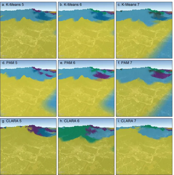
region where there is much change in the precipitation. Figure 2.9 presents an example running from the French Broad Valley bottom in Asheville, North Carolina to the ridgelines of the Black Mountains and Mt. Mitchell in the background. The K-Means 7, PAM 7, and CLARA 7 patterns are difficult to interpret because of the unrealistic number of clusters. It is unlikely that three or more hydroclimatic regions are present over the short transect distance from the valley bottom up to the ridge tops. The clusters are also highly interdigitated and patchy across the steeper slopes in the background, insinuating that multiple hydroclimatic regimes are present in similar
33
Figure 2.9: Geovisualizations of the nine clustering results are subjectively compared across the transect. The geovisualization allows the user to pan, zoom, and tilt across different topographic regions of the
SAM. Photographic imagery Copyright 2016. Image: Landsat. Data: SIO, NOAA, U.S. Navy, NGA, GEBCO.
34
Smoky Mountains, Balsam and Black Mountain ranges. Region three is located across portions of the low-lying French Broad, Tennessee, and New River valleys. Further southeast, region four contains the Blue Ridge Escarpment and extends a short distance into the North
Carolina-Virginia Piedmont. The Piedmont is denoted as region five because it spans across portions of central North Carolina, Virginia, and Tennessee. Region five also contains a disjoined area, which is separately located in the Tennessee valley, and shares similar precipitation
characteristics to the Piedmont. Given its superior performance in the CV and alignment of regions with topographic features, we choose PAM 5 results to depict the regional patterns of precipitation.
Figure 2.10: PAM 5 clustering results with 5 number of clusters or hydroclimatic regions.
35
multiple characteristics of the clusters in the visualization (Figure 2.11). This technique combines both visual and computational methods as a means of knowledge discovery in the visualization (Koua et al. 2006). It shows a relative difference in the average occurrence of each precipitation event type for the specific regions. For each plot, precipitation event types are paired across the matrix on the x and y axes, and each region is symbolized using a different color scheme. The scatterplot matrices effectively portray how the precipitation attributes of the topographic regions are distinguished from each other.
Figure 2.11: Scatterplot matrices provide a relative comparison of the average number of days per season that different precipitation event types occur. Comparisons of very light (VL), light (L), moderate
36
Figure 2.12summarizes the findings of this study in a form that effectively conveys the differences in the hydroclimatic regimes across the regions. The average Z-score of each
precipitation event type is computed for each region to reveal its hydroclimatic character, which is explored along with the regions in the visualization. Each region is also given a descriptive name that characterizes the underlying topographic environment. Regions are described in order of their geographic location from northwest to southeast. First, the NW Slopes and Plateau region is located along the northwestern boundary of the SAM and encompasses the Allegheny Plateau, Cumberland Plateau, and the Great Smoky Mountains. It exhibits relatively high
standardized frequencies of light and moderate precipitation and low standardized frequencies of very light and heavy precipitation.
The adjacent Interior Highlands region displays the highest elevations and includes portions of the Balsam and Black Mountain ranges, Great Smoky Mountains, and the Blue Ridge Escarpment. Relative to the other regions, very light and light precipitation occur more
frequently there compared to the moderate or heavy events. This finding is supported by Konrad (1996), who found a strong correlation between elevation and light precipitation, and weaker relationships between elevation and moderate or heavy precipitation.
37
many directions by mountain slopes. Moderate precipitation thus occurs seven days per season on average and heavy precipitation occurs one day per season on average.
The remaining two hydroclimatic regions are situated along the southeastern side of the SAM. The Blue Ridge and Foothills region is marked by contiguous and steep, southeastern facing slopes which extend into the adjacent Piedmont region. All precipitation event types are frequent in the Blue Ridge and Foothills region. Heavy precipitation occurs most frequently in this region compared to the others. In the Piedmont region, very light and light precipitation events are the least frequent compared to the other hydroclimatic regions. Moderate precipitation is more frequent than in the Elevated Valleys, occurring almost eight days per season on average. The Piedmont region has the second highest occurrence of heavy precipitation events.
Figure 2.12: Bar plots are used to determine the precipitation characteristics for each hydroclimatic region. Average Z-scores for each precipitation event type across the hydroclimatic regions are computed
38 Conclusions
CV is an emerging geovisualization technique that is suited to identifying patterns from large geospatial data sets. Improved computing power in recent decades has greatly increased the ability of researchers to produce a variety of maps, plots, and 3+ dimensional models using these data. However, the interpretation and communication of research that is generated using these data sets remains challenging. A substantial problem is that the increased dimension and size of geospatial data have also increased the complexity of patterns and features that are in need of interpretation. Researchers must therefore critically assess the methods that they use to simplify complex patterns into interpretable components.
In this study, we presented a detailed example of CV as a useful step in the interpretation and communication of complex hydroclimatic patterns in the southern Appalachian Mountains (SAM). The SAM is a mid-latitude mountain region located in the southeastern U.S. that exhibits much hydroclimatic and topographic variability. We used simple raster-based visualizations in Google Earth to readily discern different aspects of precipitation patterns across the region and determine how they are related to topographic patterns. Initially, we computed average summer season precipitation and the seasonal frequencies of different precipitation event types to illustrate the spatial variability in the precipitation regime across the landscape. We created a visualization of the return period for each precipitation event type to enhance the interpretability of the precipitation patterns.
39
them as input to three different partitioning algorithms. We compared five, six, and seven cluster results using internal cluster validation in order to provide a quantitative evaluation of each algorithm’s performance. Clustering results were viewed in a geovisualization, which allowed us to subjectively compare results from the nine scenarios across the landscape.
40
CHAPTER 3: RELATING WARM SEASON HYDROCLIMATIC VARIABILITY IN THE SOUTHERN APPALACHIANS TO SYNOPTIC WEATHER PATTERNS USING
SELF-ORGANIZING MAPS
Introduction
Mountains are the water towers of the world, supplying a large portion of freshwater resources to surrounding lowland regions (Messerli et al. 2004; Viviroli et al. 2007). However, the hydroclimatology of mountain regions remains poorly understood, particularly in the context of climate variability and change (de Jong et al. 2009). Observations indicate that drought and heavy precipitation have increased in the mid-latitudes during the last century (Hartmann et al. 2013), and future projections show a continuation of these trends (Christensen et al. 2013). Although research has linked increased hydroclimatic variability with changes in atmospheric circulation (Li et al. 2011; Diem 2013), our understanding of the synoptic patterns and their influence on precipitation events in mountain regions remains limited. Identifying the primary circulation patterns that are associated with different types of precipitation events and revealing how these vary across the complex terrain in mountain regions is therefore a vital component to improve future model projections.
41
Second, 500 hPa geopotential height (GPH) and mean sea level pressure (MSLP) atmospheric reanalysis fields are used in a self-organizing map (SOM) to identify the daily circulation patterns that are associated with the warm-season hydroclimatic regime. Daily
precipitation patterns are then linked with the occurrence of each circulation pattern in the SOM. Synoptic Scale Circulation Controls on Precipitation in Mountains
Synoptic-scale circulation features exert a strong control on daily precipitation by affecting the stability of the lower tropospheric air column and regulating moisture transport across the SEUS. The most important feature is the North Atlantic Subtropical High (NASH), a broad scale ridge of high pressure centered off the east coast of North America (Kam et al. 2014). Though the NASH is a semi-permanent feature from the surface through the middle troposphere, its orientation and movement influences the positioning of large scale ridge and trough patterns in the middle troposphere across North America (Wang et al. 2010; Li et al. 2011). When the NASH is displaced to the northwest of its climatological position, middle tropospheric ridging is present across the SAM, resulting in below normal precipitation amounts (Diem 2013). Likewise, displacement of the NASH to the southeast of its climatological position is tied to the occurrence of troughing and above normal precipitation amounts. The duration of hydroclimatic regimes is also related to the persistence of features, as a stationary pattern of ridging results in persistent dry periods, while a stationary pattern of troughing results in persistent wet periods (Diem 2006).
42
middle troposphere dictate the extent of rainfall over an area. In some cases, thunderstorms are organized into mesoscale convective systems (Doswell et al. 1996) that often weaken as they approach and cross portions of the SAM. These systems can occur immediately downstream (i.e. east) of a middle tropospheric short wave trough, and in the region of northwesterly flow
between a large upstream ridge and downstream trough (Konrad 1997). In addition, spatial patterns of precipitation are mediated by the geometry and orientation of features in the local scale topography (Lin et al. 2001).
Spatiotemporal Patterns of Precipitation
43
Precipitation in mountain regions is also characterized by much temporal variability. The hydroclimate regime across the SEUS is changing, with longer and more frequent dry periods found along with an increase in heavy precipitation events (Labosier and Quiring 2013). Several studies support this finding. Li et al. (2011) found that summer rainfall variability intensified over the last 30 years. Specifically, the frequency of light (0.1 - 1 mm per day) and medium (1 - 10 mm per day) rainfall events decreased and coincided with an increase in the frequency of heavy rainfall events (>10 mm day) (Wang et al. 2010). Recent research suggests that the increased rainfall variability is directly influenced by both variations in atmospheric humidity (Diem 2013), and changes in the location and movement of primary circulation components, including the NASH, over the SEUS (Li et al. 2012).
44 Study Area – Southern Appalachian Mountains
The SAM region is a mid-latitude mountain environment in the SEUS with much hydroclimatic variability and topographic complexity. Although the warm season,
lower-tropospheric circulation prevails from the southwest over the SAM, it displays much day-to-day variability (e.g. from northwesterly to southeasterly). The northwest portion of the SAM is generally wetter under northwesterly low level flow due to orographic lifting. In the southeast portion of the SAM, southerly to easterly low level flow encourages precipitation through orographic lifting or orographically mediated convection. The direction of low level flow thus influences whether topographic features are exposed to moisture advection from the Atlantic Ocean and Gulf of Mexico or rain shadowed.
The SAM is divided into four physiographic regions. (1) The Allegheny and Cumberland Plateaus are located along the northwestern boundary of the SAM, including portions of western Virginia and West Virginia (Figure 3.1, index numbers 1 and 2). The plateaus are regions of mean high elevation (>500 m), which are intersected by several stream networks. Average summer precipitation is 400 mm as a result of the northwestern exposure on the plateaus. The plateaus are therefore relatively wet compared to the adjacent valley bottoms in the Ridge and Valley region and they are hereafter collectively referred to as the northwest slopes and plateau (Table 3.1). (2) The Ridge and Valley region is located further towards the southeast and runs along the interior of the SAM through portions of Tennessee and Virginia. It is characterized by a series of relatively long, straight ridgelines running from southwest to northeast, with
45
valleys. Average summer precipitation totals are similar to the plateaus atop the ridgelines (400 mm). However, the intervening valleys are rain shadowed and thus blocked from moisture advection in nearly every direction. As a result, some portions of the New River and Tennessee valleys receive less than 254 mm of precipitation.
46
Figure 3.1: Study area map of the southern Appalachian Mountain (SAM) region depicting (a.) elevation and (b.) average summer precipitation. Important physiographic features across the SAM are also
highlighted, including (1) the Allegheny and (2) Cumberland Plateaus, (3) New River Valley, (4) Tennessee Valley, (5) Great Smoky Mountains, (6) Balsam Range, (7) Black Mountains, (8) Blue Ridge
Escarpment, and (9) North Carolina-Virginia Piedmont.
Table 3.1: Physiographic features in the southern Appalachian Mountains (SAM) are referred to according to a general reference name. The physiographic features are grouped according to their index
number, identified in in Figure 3.1.
Index
Number Physiographic Feature(s) General Reference Name
1,2 Allegheny Plateau, Cumberland Plateau Northwest Slopes and Plateau 3,4 New River Valley, Tennessee Valley Intervening Valleys
5,6,7 Great Smoky Mountains, Balsam Range,
Black Mountains Interior Highlands
8 Blue Ridge Escarpment Blue Ridge and Foothills
47 Data
Daily 500 hPa GPH and MSLP data are extracted from the European Centre for Medium-Range Weather Forecasts (ECMWF) ERA-interim reanalysis (Dee et al. 2011). ERA-Interim is a global atmospheric reanalysis available from 1979 to present, which resolves atmospheric and surface variables at ~80 km resolution across 60 vertical levels (Berrisford et al. 2011). The reanalysis fields provide a multivariate, spatially complete, and coherent record of atmospheric circulation (Dee et al. 2011). In recent years, reanalysis datasets have drastically improved due to the increased quality and coverage of observational input data.
In this paper, synoptic features in the lower and middle tropospheric circulation across the SEUS are identified and related to patterns of precipitation. 500 hPa GPH and MSLP data were downloaded across a quadrangle from 27.3° N to 40.8° N in latitude and 91° W to 72° W in longitude. The spatial domain includes much of eastern North America, as well as portions of the Gulf of Mexico and the western Atlantic Ocean (Figure 3.2). Data were obtained at 6-h intervals and averaged every 24-h period from 00Z to 00Z for the months June, July, and August over the period 1979 – 2014.
48
we recognize that each grid cell provides an average aerial estimate of precipitation. Daily data were collected for this study from 2002 - 2014 for the months of June, July, and August.
Figure 3.2: The spatial domain used in this study includes a broad quadrangle across the southeastern U.S. (SEUS). Geopotential height (GPH) and mean sea level pressure (MSLP) fields are extracted from the ERA-Interim using this domain. Grid cells are outlined using light grey. Daily PRISM precipitation fields are also extracted over the southern Appalachian Mountain (SAM) study area (dark rectangle).
Implementation of the Self-Organizing Map (SOM)
49
We employ a sequential training scheme for the SOM. Circulation patterns are randomly selected from the data space through an automated procedure and placed onto the network of nodes in the array (Kohonen 1997; Wehrens and Buydens 2007). The size of the array is subjectively determined based on the amount of detail or generalization that is desired between patterns. Each node is then assigned a reference vector coefficient and the remaining daily
circulation patterns are sequentially presented to the map. Each node is updated to reflect the best matching units, which are closest in the data space, allowing the map to self-organize until the final arrangement of circulation patterns is present. The SOM thus trains until there are no more changes in node locations within the array (Hewitson and Crane 2002). At this stagnation threshold, the nodes in the array provide a theoretical representation of atmospheric circulation, which can then be related to the different types of precipitation events. Individual circulation patterns from the original data may therefore contribute to the pattern that is present in one or more nodes. The nodes are not discrete, but rather comprised of all possible circulation patterns that exhibit similarity to the specific node in that area of the SOM-space. For further discussion of the various implementations of the SOM in synoptic climatology, we refer the reader to Hewitson & Crane (2002), Sheridan & Lee (2011), and Skific & Francis (2012).
There are two major benefits of the SOM over traditional types of synoptic classification. First, the SOM is more versatile. No assumptions about the data have to be made in advance to run the classifications (Yarnal et al. 2001). Second, the SOM is a spatially-organized
50
regimes that exhibit much similarity tend to be located adjacent to one another. While these theoretical patterns may be minimally present in the observations, they provide a relation to the surface phenomena because all possible configurations of pressure patterns are visible in the array (Hewitson and Crane 2002).
Classification of the Synoptic Scale Circulation
Daily atmospheric circulation patterns are classified over the SEUS from 1979 – 2014 using a 3x4 SOM with 12 nodes. A 4x4 and a 4x5 SOM with 16 and 20 nodes, respectively, are also trained to compare the distribution of circulation patterns in different sized arrays. Although the larger-sized SOMs increase the number of circulation categories in the array, they reduce the amount of change in the patterns from node-to-node. Circulation patterns belonging to the same neighborhood of nodes in the array are often indistinguishable, which limits the ability to draw conclusions about the variability between circulation patterns. The 3x4 SOM with 12 nodes, on the other hand, increases variability between the nodes and retains visually interpretable
differences in the circulation from node-to-node.
To emphasize patterns in the middle troposphere, the SOM is trained using daily ERA-Interim 500 mb GPH data over 36 summer seasons (Figure 3.3). The patterns aggregated in the SOM-space thus represent 3312 circulation days over the SEUS. In order to incorporate the low level flow, MSLP fields are composited by taking an average of the days assigned to each node (Figure 3.4). The frequency of each circulation pattern is computed as a percentage of time that the identified pattern is present during the summer time. The frequencies are then displayed in each node across the SOM.
51
column combination, or simply by groups of patterns according to row or column. There are a wide range of circulation patterns identified across the SOM over the SEUS during the study period. In general, middle tropospheric troughs are positioned upstream or over the SAM along the left side of the SOM (i.e. columns A and B) and ridging patterns are located over or upstream of the SAM along the right side of the SOM (i.e. columns C and D). The corresponding
composite surface patterns feature a surface wave and trailing front, with low pressure across the SAM (columns A and B), and high pressure across the domain in association with the northwest ridge of the NASH (columns C and D).
We summarize the middle tropospheric circulation and corresponding surface pressure patterns in a clockwise fashion around the SOM. The row 3 maps reveal variations in the positioning of a ridge from overhead in column D3 to downstream in D1. The corresponding MSLP composites depict a strong NASH centered immediately east of the region in D3 to a much weaker NASH situated far off the coast in A3, along with the approach of a surface front from the northwest. The map patterns in the third row are present on roughly 45% of the days during the summer, with node B3 occurring the most frequently.
52
53
Figure 3.3: Self-organizing map (SOM) trained from ERA-Interim daily 500 mb geopotential height (GPH) fields for the warm season during the period 1979 – 2014. Nodes are referenced according to their row and column combination. For example, node D3 refers to the lower right corner of the
54
Figure 3.4: Composited mean sea level pressure (MSLP) is calculated based on the days assigned to each node in the self-organizing map (SOM). The MSLP contour interval is 1 hPa for each node.
The Hydroclimate of the SAM and its Relationship with Circulation Patterns
55
determined for each node by calculating the percentage of days in which each precipitation event type occurs over each grid cell in the SAM.
The frequency of each of the precipitation event types across the SAM is presented in Figure 3.5. Dry days with no precipitation are the most frequent during the summer time,
occurring greater than 50% of the time across the majority of the SAM and up to 65% of the time in the intervening valleys and Piedmont. Along the interior highlands and Blue Ridge and
foothills, dry days occur least frequently (<40%).
Days with very light and light precipitation are the second most frequent during the summer time. Very light precipitation occurs on nearly 20% of days across the interior highlands and up to 25% of days on the most exposed areas of the southern Blue Ridge and foothills. Light precipitation is also more frequent throughout these regions. It occurs on up to 30% of days in the interior highlands and southern Blue Ridge and foothills regions. These two precipitation event types collectively account for more than half of the summer precipitation climatology across the high elevation areas of the SAM. Very light and light precipitation occur least frequently (e.g. <15%) throughout the intervening valleys and across the Piedmont.
Days with moderate or heavy precipitation occur least frequently across the SAM, although several topographic gradients are present. The maximum frequency of moderate
56
intervening valleys. In contrast, it occurs up to 4% of days along the southern Blue Ridge and foothills region and 2% of days in places throughout the Piedmont.
There are a wide range of circulation patterns that are linked with the occurrence of each precipitation event type across the different physiographic regions of the SAM. In general, each of the precipitation event types occur with the greatest frequency in the left and lower left
57
Figure 3.5: The frequency of days with (a.) none, (b.) very light, (c.) light, (d.) moderate, and (e.) heavy rainfall in the southern Appalachian Mountains (SAM) during the warm season over the period 2002 –
2014. The frequency of each precipitation event type is denoted as a percentage of time.
58
in the intervening valleys and Piedmont and least frequently (10 - 20% of the time) across the interior highlands, northwest slopes and plateau, and along the Blue Ridge and foothills.
Figure 3.6: Days with no rainfall are plotted in the self-organizing map (SOM) based on their occurrence as a percentage of time when the associated circulation patterns are present from node to node.
59
places in the intervening valleys, Piedmont, and various smaller valleys which bisect the interior highlands.
Figure 3.7: Days with very light rainfall are plotted in the self-organizing map (SOM) based on their occurrence as a percentage of time when the associated circulation patterns are present from node to
node.
60
occurs with the least frequency in connection with northwesterly to west northwesterly flow (i.e. ridge upstream or over the region). Days with light rainfall in this part of the SOM occur with the greatest frequency (20 - 30% of the time) throughout the interior highlands and some isolated areas of the northwest slopes and plateaus and southern Blue Ridge and foothills. They are least frequent in the intervening valleys and Piedmont, occurring less than 20% of the time.
Figure 3.8: Days with light rainfall are plotted in the self-organizing map (SOM) based on their occurrence as a percentage of time when the associated circulation patterns are present from node to
node.
61
parts of the Blue Ridge and foothills along the North Carolina-Virginia border. It occurs least frequently (10 - 20% of the time) throughout the interior highlands, intervening valleys, and the northwestern slopes and plateaus. Moderate rainfall events occur least frequently in association with the patterns of northwesterly flow found in the middle to upper right section of the SOM space. It was most frequent (10 - 20% of the time) along some of the northwestern slopes and plateaus and in a few places in the interior highlands. It was least frequent (less than 10% of the time) in the remaining regions of the SAM, including the intervening valleys, Blue Ridge and foothills, and Piedmont.
Figure 3.9: Days with moderate rainfall are plotted in the self-organizing map (SOM) based on their occurrence as a percentage of time when the associated circulation patterns are present from node to