DOI:10.1051/0004-6361/201220717 c
ESO 2013
Astrophysics
&
Outflow forces of low-mass embedded objects in Ophiuchus:
a quantitative comparison of analysis methods
N. van der Marel
1, L. E. Kristensen
1,2, R. Visser
3, J. C. Mottram
1, U. A. Yıldız
1, and E. F. van Dishoeck
1,41 Leiden Observatory, Leiden University, PO Box 9513, 2300 RA Leiden, The Netherlands e-mail:[email protected]
2 Harvard-Smithsonian Center for Astrophysics, 60 Garden Street, Cambridge, MA 02138, USA 3 Department of Astronomy, University of Michigan, 500 Church St., Ann Arbor, MI 48109-1042, USA 4 Max-Planck-Institut für Extraterrestrische Physik, Giessenbachstrasse 1, 85748 Garching, Germany
Received 11 November 2012/Accepted 27 May 2013
ABSTRACT
Context.The outflow force of molecular bipolar outflows is a key parameter in theories of young stellar feedback on their surround-ings. The focus of many outflow studies is the correlation between the outflow force, bolometric luminosity, and envelope mass. However, it is difficult to combine the results of different studies in large evolutionary plots over many orders of magnitude due to the range of data quality, analysis methods, and corrections for observational effects, such as opacity and inclination.
Aims.We aim to determine the outflow force for a sample of low-luminosity embedded sources. We quantify the influence of the analysis method and the assumptions entering the calculation of the outflow force.
Methods.We used theJames Clerk MaxwellTelescope to map12COJ =3–2 over 2×2 regions around 16 Class I sources of a well-defined sample in Ophiuchus at 15resolution. The outflow force was then calculated using seven different methods differing, e.g., in the use of intensity-weighted emission and correction factors for inclination. Two well studied outflows (HH 46 and NGC1 333 IRAS4A) are added to the sample and included in the comparison.
Results.The results from the analysis methods differ from each other by up to a factor of 6, whereas observational properties and choices in the analysis procedure affect the outflow force by up to a factor of 4. Subtraction of cloud emission and integrating over the remaining profile increases the outflow force at most by a factor of 4 compared to line wing integration. For the sample of Class I objects, bipolar outflows are detected around 13 sources including 5 new detections, where the three nondetections are confused by nearby outflows from other sources. New outflow structures without a clear powering source are discovered at the corners of some of the maps.
Conclusions.When combining outflow forces from different studies, a scatter by up to a factor of 5 can be expected. Although the true outflow force remains unknown, the separation method (separate calculation of dynamical time and momentum) is least affected by the uncertain observational parameters. The correlations between outflow force, bolometric luminosity, and envelope mass are further confirmed down to low-luminosity sources.
Key words.ISM: jets and outflows – ISM: molecules – stars: protostars – stars: low-mass – circumstellar matter – submillimeter: ISM
1. Introduction
Molecular outflow activity begins early during the formation process of low-mass protostars and is therefore a tracer of ac-tive star formation (Bachiller & Tafalla 1999;Arce & Sargent 2006). Outflows actively contribute to the core collapse and for-mation of the star by carrying away angular momentum that would otherwise prevent accretion (Bachiller 1996;Hogerheijde et al. 1998). The strength of an outflow is measured by the out-flow forceFCO: the ratio of the momentum and the dynamical
age of the outflow (Bachiller & Tafalla 1999). It is a measure of the rate at which momentum is injected into the envelope by the protostellar outflow (Downes & Cabrit 2007). The outflow force has been used to understand the driving mechanism of outflows. The correlation between the bolometric luminosityLboland
out-flow force suggests that a single mechanism is responsible for driving the outflow, at least partly related to accretion (Cabrit & Bertout 1992). A second correlation between FCO andMenv
Appendices are available in electronic form at
http://www.aanda.org
(Bontemps et al. 1996) underlines the evolutionary properties of this parameter, suggesting that the outflow activity declines during the later stages of the accretion phase though this is more difficult to separate from initial conditions (Hatchell et al. 2007). Due to these correlations, the outflow force is a very important parameter for understanding the physical processes underlying the early phases of star formation.
Outflow forces have been derived for many embedded sources over the past 30 years using various methods and with a continuous increase in observational resolution and signal-to-noise ratio (S/N), resulting in a very inhomogeneous data set. Outflow properties for low-mass protostars have been compared in population studies of entire star forming regions and in dif-ferent phases of evolution, ranging from the deeply embedded Class 0 to the T Tauri Class II stage (Cabrit & Bertout 1992; Bontemps et al. 1996;Richer et al. 2000;Arce & Sargent 2006; Hatchell et al. 2007). A central focus of many of these studies is the evolutionary trend plots ofFCOversusLbolandFCO
ver-susMenvas described above. However, the results of these
stud-ies cannot usually be combined into a single dataset that includes
all nearby clouds due to the range of data quality, the different methods used to determine outflow properties, and the different corrections for observational effects that have been applied, such as opacity and inclination.
For individual targets, different methods have been shown to result in different values of the outflow force up to an or-der of magnitude (Hatchell et al. 2007). Comparisons of the value of the outflow force with different CO transitions (e.g. J=1–0, 2–1, 3–2, 6–5) show similar results (van Kempen et al. 2009a;Nakamura et al. 2011;Yıldız et al. 2012). Although some comparison studies with outflow models exist (Cabrit & Bertout 1992, CB92 hereafter; Downes & Cabrit 2007, DC07 hereafter), the influence of the analysis method itself and the assumptions entering the calculation have never been quantified systemati-cally against a single set of observational data.
The ρ Oph molecular cloud complex (d ∼ 120±4 pc; Loinard et al. 2008) is one of the nearest and best-studied star forming regions (Lada & Wilking 1984; Greene et al. 1994). Tens of young stellar objects (YSOs) have been identified, es-pecially in the main filament L1688 (Wilking et al. 2008, and references therein). Due to the clustering of star formation in Ophiuchus, the YSOs are very close together and their out-flows sometimes overlap along the line of sight (e.g.Bussmann et al. 2007). Class I outflows in Ophiuchus have been studied extensively and their properties have been obtained for many sources (Bontemps et al. 1996;Sekimoto et al. 1997;Kamazaki et al. 2001,2003;Ceccarelli et al. 2002;Boogert et al. 2002; Bussmann et al. 2007;Gurney et al. 2008;Zhang & Wang 2009; Nakamura et al. 2011). Additional studies of YSOs in Ophiuchus from earlier data, including sources with outflows, are summa-rized inWilking et al. (2008). It has been suggested that star formation in Ophiuchus was triggered by supernovae, ionization fronts and winds from the Upper Scorpius OB association, lo-cated to the west of the Ophiuchus cloud (Preibisch & Zinnecker 1999;Nutter et al. 2006) and started in the denser northwestern L1689 region (Zhang & Wang 2009).
In a recent study byvan Kempen et al. (2009c), a number of YSOs in Ophiuchus were classified as so-called “Stage 1” sources, using a new classification based on Mdisk, Menv
andMstar. Since this classification relies on physical rather than
observational parameters (cf. Lada classification, with spectral slopeαIR,Lada & Wilking 1984), this sample represents a
well-defined embedded YSO sample in this cloud and outflow ac-tivity is expected to be detected from every source. For about half of these sources bipolar outflows were identified previ-ously, but not with the high spatial resolution of 15 that is available with the HARP array receiver (Buckle et al. 2009) at the James Clerk Maxwell Telescope (JCMT). High-resolution
12CO J=3–2 spectral maps offer the means to study the
oc-curence, origin and properties of the outflows in more detail than previous studies. Therefore, this data set is perfect to systemati-cally study and quantify the effect of different analysis methods. The sources are also part of theHerschelkey programs “Water in Star-forming Regions withHerschel” (WISH) and “Dust, Ice and Gas In Time” (DIGIT;van Dishoeck et al. 2011; Green et al. in prep.): complementary data on feedback based on far infrared line emission will become available in the following years for comparison.
This paper presents the results of a comparison between analysis methods of the outflow force with CO spectral maps, applied to 13 sources in Ophiuchus and two additional, well-studied outflows: HH 46 (van Kempen et al. 2009a) and NGC 1333 IRAS4A (Yıldız et al. 2012). The outline of this paper is as follows. In Sect. 2, the details of the observations
and basic data reduction are discussed. Section 3 presents the spectral profiles and contour maps of the integrated line wings, indicating the outflow lobes. In Sect. 4, the results of the vari-ous outflow force analysis methods are presented and discussed. Section 5 discusses the comparison of outflow force values with those found in the literature, the trends of the outflow parameters and its implications for evolutionary models and the comparison of outflow morphologies with observed disks. The conclusions of the paper are given in Sect. 6.
2. Observations
2.1. Sample selection
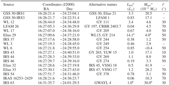
The 16 “Stage 1” sources identified by van Kempen et al. (2009c) were selected for the sample of this outflow study, out of a sample of 41 sources with potential Class I classifica-tion (α2−24μm > 0.3 and Tbol <650 K). Figure1 presents an
overview of our sample, the basic properties of which are shown in Table1. IRS 46 is classified as Stage 2, but an outflow was also detected for this source in this study. TheLbolfor this
sam-ple ranges from 0.04 to 14.1L. Except for IRS 63, all sources are located in the L 1688 ridge.
Figure 1 shows an overview of the bipolar outflows and their relative positions in the L1688 core in Ophiuchus, where each square represents a spectral map and the red and blue ar-rows show the direction and extent of the red and blue outflows. VLA 1623 is added as well, based on figures inYu & Chernin (1997). The background shows the 850μm SCUBA map as pub-lished byJohnstone et al.(2000) andDi Francesco et al.(2008). IRS 63 lies outside the borders of this map and is presented as inset.
2.2.12CO maps of Ophiuchus
All sources were observed in the J = 3–2 line of 12CO
(345.796 GHz) with the HARP array receiver at theJames Clerk MaxwellTelescope (JCMT) as part of program M08AN05. A bandwidth of 250 MHz was used with the ACSIS backend, re-sulting in a native spectral resolution of 0.026 km s−1. The
obser-vations were carried out in June 2008 under weather conditions with an atmospheric opacityτ225GHzranging from 0.08 to 0.12.
For analysis of the line wings, the spectra are typically binned to 0.1 km s−1, givingσ
rms = 0.2 K. The HARP array consists
of 16 receivers arranged in a 4×4 pattern, mapping the sources over 2×2to capture the full extent of the outflows with 15 spatial resolution. The maps were made in the jiggle observing mode and resampled with a pixel size of 7.5. A position switch of 60or 150was used. For one night, the reference off posi-tion accidentally coincided with emission, resulting in negative absorption troughs in the spectra in the maps of Elias 32 and Elias 33, IRS 37, IRS 43, IRS 44, LFAM 26, WL 17 and IRS 54. This has, however, no influence on the study of line wings. The Class 0 source IRAS 16293–2422 was used as a line calibrator. The main-beam efficiency was 0.631 and pointing errors were
within 2. Two receivers were broken at the time of observa-tion (H03 and H014), resulting in lack of data in the southeast and the north-northwest corner of each map. Some sources are separated by less than 30 and were therefore mapped in a sin-gle image (Elias 32+Elias 33; IRS 37+WL 3; GSS30-IRS1+ GSS30-IRS3; and IRS 44+IRS 46). Only for the last case could the two sources be analyzed separately. In addition, Elias 33 was 1 http://www.jach.hawaii.edu/JCMT/spectral_line/
Fig. 1.L1688 core in Ophiuchus and the region around IRS 63 (inset upper left corner). The background shows the 850μm SCUBA map (Johnstone et al. 2000;Di Francesco et al. 2008). The locations of all observed HARP maps are indicated by squares, labeled by the sources within. The blue and red arrows indicate the direction and observed extent of the blue and red outflow of that source, except for the extent of VLA 1623, which was taken fromYu & Chernin(1997) who observed the region centered on VLA 1623. In crowded regions, lines connect the source names to the origin location of the outflow. Newly detected outflow structures without a driving source are marked with Us.
Table 1.Sample of Stage 1 sources in Ophiuchus.
Source Coordinates (J2000) Alternative names Lbola Menva ic
RA Dec (L) (10−2M
) (◦) GSS 30-IRS1 16:26:21.4 −24:23:04.1 GSS 30, Elias 21 3.3 20.5 –
GSS 30-IRS3 16:26:21.7 −24:22:51.4 LFAM 1 0.83 17.1 –
WL 12 16:26:44.0 −24:34:48.0 GY 111 3.4 4.6 30
LFAM 26 16:27:05.3 −24:36:29.8 GY 197, CRBR 2403.7 0.04 4.5 70
WL 17 16:27:07.0 −24:38:16.0 GY 205 0.67 4.0 50
Elias 29 16:27:09.6 −24:37:21.0 WL15, GY 214 14.1b 4.0b 50
IRS 37 16:27:17.6 −24:28:58.0 GY 244 0.38 1.2 50
WL 3 16:27:19.3 −24:28:45.0 GY 249 0.46 2.9 –
WL 6 16:27:21.8 −24:29:55.0 GY 254 0.85 <0.4 50
IRS 43 16:27:27.1 −24:40:51.0 GY 265, YLW 15 1.0 17.1 10
IRS 44 16:27:28.3 −24:39:33.0 GY 269 1.1 8.0 30
IRS 46 16:27:29.7 −24:39:16.0 GY 274 0.19 3.3 50
Elias 32 16:27:28.6 −24:27:19.8 IRS 45, VSSG 18 0.5 41.9 – Elias 33 16:27:30.1 −24:27:43.0 IRS 47, VSSG 17 1.2 28.2 70
IRS 54 16:27:51.7 −24:31:46.0 GY 378 0.78 3.1 50
IRAS 16253–2429 16:28:21.6 −24:36:23.7 0.06 10.3 70
IRS 63 16:31:35.7 −24:01:29.5 GWAYL 4 1.0b 30.0b 30
Notes.(a)Parameters taken fromvan Kempen et al.(2009c), unless indicated otherwise.(b)FromKristensen et al.(2012).(c)Estimates from this work, see Sect.4.2.
observed in September 2007 with HARP in the raster observ-ing mode. This source was mapped in a 4×4 region and re-sampled to a pixel size of 12. Atmospheric opacity was 0.05. The rms noise σrms for the rebinned spectra is again 0.2 K
in 0.1 km s−1bins.
2.3.13CO spectra
In order to determine the optical depth of the line wings of the outflows additional13COJ = 3–2 (330.58797 GHz)
spec-tra were taken for two of the strongest outflows (Elias 29
and IRS 44) at the central positions. The HARP array receiver at the JCMT was used in the same setup as the12CO observations as single pointings instead of jiggle maps. The observations were carried out in March 2011 as part of program M10BN05 under weather conditions with an opacityτ225 GHz of∼0.11. The rms
noiseσrmsfor the reduced spectra is 0.05 K in 0.4 km s−1bins.
Fig. 2.12CO 3–2 spectra toward IRS 63, from top to bottom: one red outflow lobe position (15, 15), one blue outflow lobe position (0, −7.5), the central position (0, 0) and one off-source position (−42.5, 20). The integration limits are marked by dotted lines, baselines by dash-dotted lines and the source velocity by a dashed line.
2.4.12CO maps of HH46 and IRAS4A
For the outflow analysis comparison,12CO J = 3–2 datasets published invan Kempen et al.(2009a) andYıldız et al.(2012) of HH 46 and IRAS4A were used, respectively. The HH 46 ob-servations were taken at the Atacama Pathfinder EXperiment (APEX), regridded to a map of 2×2 and have a typical rms noise of 0.6 K in 0.2 km s−1bins. The observations of IRAS4A were taken in jiggle mode with the HARP array receiver at the JCMT, regridded to a map of 4×4have a typical rms noise of 0.15 K in 0.1 km s−1bins. For more details on these
observa-tions, see the original references.
3. Results
3.1. Spectral profiles
12COJ = 3–2 is detected towards all sources, showing broad
line profiles centered on LSR ∼ 4 km s−1. An example set
of spectra is shown in Fig. 2 for IRS 63. The spectral pro-files consist of red/blue-shifted wing emission from the out-flow, central emission peaks from cloud and envelope material or foreground layers and narrow absorption features caused by self-absorption. At the outflow positions, broad line wings are detected, up to+15 km s−1in the red and−10 km s−1in the blue.
3.2. Outflow maps
Outflow maps were made of the integrated CO wing emission in blue and red velocity intervals. The integration limits were chosen as follows. For each position, the outer velocity,out,
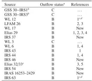
Table 2.Outflow status for the 16 sources in this sample.
Source Outflow statusa References
GSS 30−IRS1b C . . .
GSS 30−IRS3b C . . .
WL 12 B 1c,d
LFAM 26 B 2, 3
WL 17 B New
Elias 29 B 1, 2, 3, 4
IRS 37 B New
WL 3 C . . .
WL 6 B 1, 4
IRS 43 B 1
IRS 44 B 1, 4
IRS 46 B New
Elias 32/33e B 3, 5
IRS 54 B New
IRAS 16253–2429 B New
IRS 63 B 1c,d
Notes. (a) Outflow status: B for bipolar outflow and C for confu-sion because of the presence of nearby sources.(b)Outflow confusion with VLA 1623.(c) IRS 63 is named L1709B (name of the core) or 16285-2355 inBontemps et al.(1996).(d)IRS 63 and WL 12 were not recognized as bipolar inBontemps et al.(1996).(e) Due to the small separation of Elias 32 and 33, it is not clear to which source the outflow belongs. Elias 33 is assigned as the driving source in this study.
References.(1)Bontemps et al.(1996); (2) Bussmann et al.(2007); (3)Nakamura et al.(2011); (4)Sekimoto et al.(1997); (5)Kamazaki et al.(2003).
is defined as the velocity where the emission is still above the 1σrms level in 0.1 km s−1bins. The inner velocity limits,in,
in each map are defined as theout in an off-source12CO spec-trum (see Fig.2for the example of IRS 63). The blue wing in-tegration limits typically range from−6 km s−1 to+1 km s−1,
and for the red wing from 6 km s−1to 12 km s−1(see Fig.F.1).
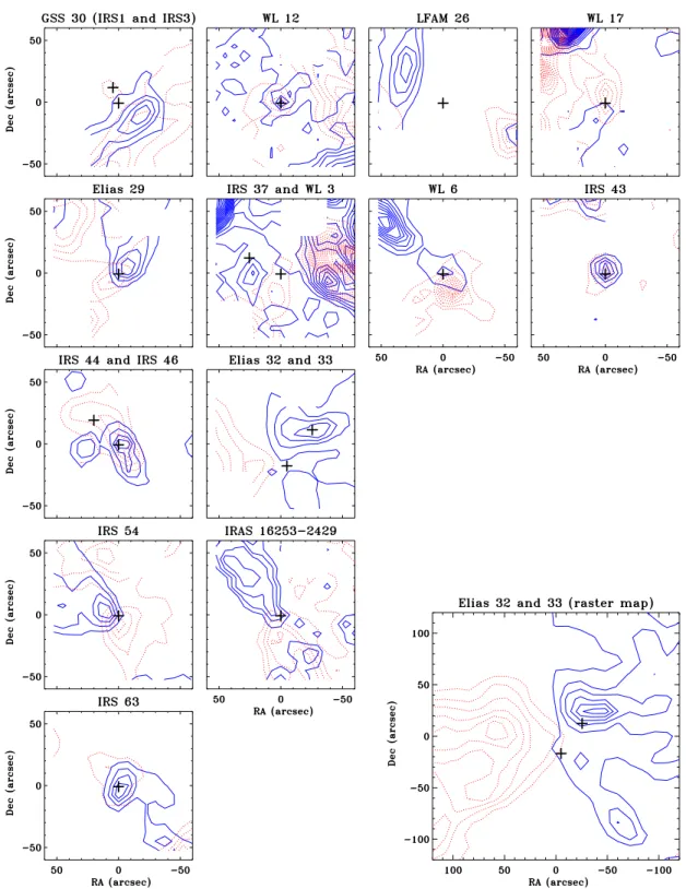
Contour maps of the integrated outflow emission are presented in Fig.3.
The maps show outflow activity in most of the sources. Infrared source positions are at (0, 0) or marked when there are multiple sources. Most outflows fit in the 2×2 region, except for Elias 32/33, Elias 29, LFAM 26 and IRAS 16253– 2429, although the outflow direction can still be recognized. Elias 32/33 is also observed in the raster mode in 4×4maps, covering a larger part of the outflow (see lower right panel in Fig.3).
Bipolar outflows are seen for 13 sources (see Table 2), al-though nearby outflows complicate the view in several cases. In the Elias 29 map, emission from the east lobe of LFAM 26 is seen in the upper right corner, while part of the blue lobe of Elias 29 falls in the LFAM 26 map and the red lobe in the WL 17 map. A full coverage of these two outflows can be found inBussmann et al.(2007) andNakamura et al.(2011). The red lobe of Elias 32/33 extends all the way to IRS 54 and the blue lobe is wide enough to show close to WL 6 (Nakamura et al. 2011). The lobes of IRS 44 extend into the IRS 43 map. In the map containing GSS 30, the outflow emission is completely dominated by the 15long outflow extending from VLA 1623, a Class 0 source at 16:26:26.26,−24:24:30.01 (Andre et al. 1993; Dent et al. 1995;Yu & Chernin 1997). A high-velocity bullet (Bachiller & Tafalla 1999) at 28 km s−1, not identified in
Fig. 3.Outflow maps of all sources. Contours are drawn based on the integrated intensities of the line wings. Contours are drawn at 20, 40, 60, 80 and 100% of the peak value of the integrated intensity of the target source. The source positions are marked by pluses. Two receivers were broken at the time of observation, resulting in lack of data in the southeast and north-northwest corner of each map. In maps with Elias 32 and 33, Elias 32 is northwest of Elias 33. In the GSS 30 map, GSS 30-IRS3 is north of GSS 30-IRS1. In the IRS 37 map, WL 3 is east of IRS 37. In the IRS 44 map, IRS 46 is northeast of IRS 44.
reveal this outflow. In the case of Elias 29 and Elias 32/33, the red and blue lobes overlap with the pixels from the broken re-ceivers, thus possibly underestimating the total outflow mass.
In the maps of Elias 32/33 and IRS 37/WL 3, only one set of outflow lobes was resolved: for this study they were assigned to Elias 33 and IRS 37, respectively. In the map of IRS 44, the Class II source IRS 46 is located 20northeast of IRS 44. Based on the sudden change of shape of the line wings, the spectral
map was cut in two, assigning one half to IRS 46 and one half to IRS 44, each with their own bipolar outflow. In the maps contain-ing IRS 37, IRS 44, IRS 63 and WL 12 new outflow structures were discovered which could not be assigned to an IR source. These structures were assigned U1, U2, etc. and are discussed further in AppendixA.
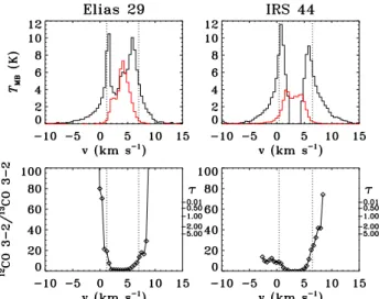
Fig. 4.12CO 3–2 and13CO 3–2 spectra of the central position of Elias 29 (left) and IRS 44 (right). The top figure shows the spectra, binned to 0.42 km s−1, thebottom figure shows theT
MB ratio of12CO 3–2/ 13CO 3–2 and the corresponding optical depthτon the right axis. The dotted lines show the integration limits, indicating the velocities in where the line wings start.
outflows were identified and nine were confirmed from previous observations.
3.3. Optical depth
The optical depth,τ, is obtained from the line ratio of12COJ=
3–2 and its isotopolog13COJ =3–2 for the central position of
the outflows with the strongest line wings, Elias 29 and IRS 44. In Fig.4, spectra of12CO J = 3–2 and13CO J = 3–2 at the central positions are shown, binned to 0.42 km s−1, together with
the ratio of12CO J = 3–2/13CO J = 3–2. The optical depth for the line wings is derived assuming that the two species have the same excitation temperature and that the13CO line wing is
optically thin, using (Goldsmith et al. 1984):
I(12CO)
I(13CO)=
1−e−τ12 1−e−τ13 ≈
1−e−τ12 τ12 ×
R (1)
withR =τ12/τ13the abundance ratio12CO/13CO (a ratio of 65
is assumed here, followingVladilo et al. 1993). The resulting optical depths of12CO as a function of velocity are shown on the right-hand axes of the lower panels of Fig.4. High optical depths>2 are found at velocities very close to the source veloc-itysourceimplying that the central velocities are optically thick and become optically thinner away from the line center where the outflow emission starts. The only exception is the blue wing of IRS 44, which remains optically thick for 3 km s−1beyondin.
Quantitatively, the optical depth implies that the mass of the blue lobe at this single position is underestimated by a factor of 6 if the wing emission is assumed to be optically thin. At the other positions with13CO measurements, the blue wing is still
opti-cally thin, so the total blue mass is not expected to increase more than a factor of 2 due to optical depth effects. Since the uncer-tainties on the outflow force are within a factor of a few, the im-pact of optical depth is negligible. Therefore outflow emission is assumed to be optically thin for all sources.
4. Outflow analysis
4.1. Outflow parameters
The main physical parameters of the outflow are the mass,M, the velocity,CO(defined as|out−source|, withoutthe outer veloc-ity of the outflow emission at a given location), and the projected size of the lobeRlobe, for both the blue and red lobe. The mass is
calculated from the integrated intensity of the12CO line
assum-ing an excitation temperature of 50 K (e.g.Yıldız et al. 2012) and the procedure explained in AppendixC. With these basic physical quantities the outflow force,FCO, can be derived as
FCO=
M2CO Rlobe ·
(2) The velocity,CO, often calledmax, is not a well-constrained pa-rameter: due to the inclination and the shape of the outflow, often following a bow shock including forward and transverse motion, the measured velocities along the line of sight are not necessarily representative of the real velocities driving the outflow (Cabrit & Bertout 1992). This is the main reason why various methods have been developed to derive the outflow force, where a correc-tion factor is often applied to compensate for these effects.
4.2. Analysis methods
Seven different methods for deriving the outflow force are an-alytically described in this section, with references to the pa-per where the method was originally presented. The constantK refers to Eq. (C.4). The following general recipe applies to each method for the blue and red lobe separately. The outflow parameters are calculated by adding up the absolute values for the blue and red lobe.
1. For each pixel, j, the outer velocityout,j is defined as the outer velocity where the emission is still above the 1σrms level.
2. The inner velocity,in, in each map is defined as the velocity in the average off-source12CO spectrum where the emission
is still above 5% of the peak emission Tpeak. in and out,j define the integration limits for each line wing, the samein is used for each pixel.
3. The source velocity, source, is determined using a high-density tracer such as HCO+or a minor isotopologue with a non-self-absorbed profile. =−sourceis defined as the relative velocity.
4. Only pixels that are contributing to the outflow of the target are included to avoid confusion with nearby outflows. 5. The inclination angle, i, is estimated from the morphology
of the contour map to be pole on (10◦), inclined (30◦or 50◦) or in the plane of the sky (70◦), using Fig. 1–4 inCabrit & Bertout(1990).
6. Rlobeis measured as the projected length of the outflow lobe.
7. The conversion from integrated intensity to mass is a multi-plication with constantKas defined in AppendixC.
4.2.1.vmaxmethod (M1)
Table 3.Correction factors.
i(◦) 10 30 50 70 Ref.
c1 0.28 0.45 0.45 1.1 1,2
c2 1.6 3.6 6.3 14 1
c3a 1.2 2.8 4.4 7.1 3
Notes.(a)The values are interpolated from the ratios in the third column of Table 6 ofDownes & Cabrit(2007), whereα=90−i.
References.(1)Cabrit & Bertout (1990), (2) CB92, (3) Downes & Cabrit(2007).
factorsc1(i) (see Table3) derived byCabrit & Bertout(1990,
1992) forCOto obtainFCO:
FCO=c1
K ⎛ ⎜⎜⎜⎜⎜ ⎜⎝ j
T()d
j
⎞ ⎟⎟⎟⎟⎟ ⎟⎠2
max
Rlobe ·
(3)
4.2.2.vspreadmethod (M2)
In M2,out,j is derived as a function of position (Yıldız et al. 2012). The local energyM2
CO,j is calculated for each position in the map with the local velocity. No correction factors are applied:
FCO=
K ⎛ ⎜⎜⎜⎜⎜ ⎜⎝ j 2 out,j×
T()d
j ⎞ ⎟⎟⎟⎟⎟ ⎟⎠ Rlobe · (4)
4.2.3.v method (M3)
M3 uses intensity-weighted velocities by includingin the in-tegral (Cabrit & Bertout 1990;Downes & Cabrit 2007). The de-rived outflow force is multiplied by the inclination correction factorsc2(i) (Table3) derived inCabrit & Bertout(1990) for
to obtainFCO:
FCO=c2×K ⎛ ⎜⎜⎜⎜⎜ ⎜⎜⎜⎜⎜ ⎜⎜⎜⎜⎜ ⎜⎜⎜⎜⎜ ⎜⎜⎜⎜⎝ ⎧⎪⎪ ⎪⎨ ⎪⎪⎪⎩j
T()d
j ⎫⎪⎪ ⎪⎬ ⎪⎪⎪⎭ 2 Rlobe j
T()d
j ⎞ ⎟⎟⎟⎟⎟ ⎟⎟⎟⎟⎟ ⎟⎟⎟⎟⎟ ⎟⎟⎟⎟⎟ ⎟⎟⎟⎟⎠ · (5)
4.2.4. Local method (M4)
Using the kinematic structure of the outflow lobe, the local out-flow force is calculated for each position by dividing the local energy M2
CO,j by the projected distancerj between the posi-tion and source posiposi-tion (Lada & Fich 1996;Downes & Cabrit 2007).Hatchell et al.(2007) use a combination of M4 and M2, using projected distances and local velocities. No correction fac-tors are applied:
FCO=K ⎛ ⎜⎜⎜⎜⎜ ⎜⎜⎜⎝j
T()2d j rj
⎞ ⎟⎟⎟⎟⎟
⎟⎟⎟⎠· (6)
4.2.5. Perpendicular method (M5)
Because a large amount of the outflow material is moving slowly and predominantly in transverse motion, DC07 developed a method to determine the dynamical age,td, of the outflow,
us-ing the half-width of the outflow lobe, Wlobe, rather than the
projected length. The factor 1
3 (see below) originates from the
asymptotic expansion of the bowshock wings,R ∝ t1/3 (DC07 and references therein). This method resulted in much more ac-curate estimates of the outflow force for the modeled outflows, but can only be applied in observations of spatially well-resolved outflows. In addition, since the models describe Class 0 sources, the results may not be applicable for outflows of Class I sources which are known to have large opening angles (e.g. Arce & Sargent 2006):
FCO=K ⎛ ⎜⎜⎜⎜⎜ ⎜⎜⎜⎜⎜ ⎜⎜⎜⎜⎜ ⎜⎜⎜⎜⎜ ⎜⎜⎜⎜⎝ ⎧⎪⎪ ⎪⎨ ⎪⎪⎪⎩j
T()d
j ⎫⎪⎪ ⎪⎬ ⎪⎪⎪⎭ 2 1 3Wlobe
j
T()d
j ⎞ ⎟⎟⎟⎟⎟ ⎟⎟⎟⎟⎟ ⎟⎟⎟⎟⎟ ⎟⎟⎟⎟⎟ ⎟⎟⎟⎟⎠ · (7)
4.2.6. Annulus method (M6)
In M6, the outflow force is calculated with a “slice” through the outflow (Bontemps et al. 1996). The momentum within an an-nulus or ring centered on the source position with thicknessΔr (equal to the beam size) and radiusris measured, and the dy-namical age is determined withΔr rather than Rlobe. The
de-rived outflow force Fobs is multiplied by a mean correction
factor f(i) = 2.9 with f(i) = sini/cos2i andi ≈ 57.3◦.
Bontemps et al. (1996) applied an additional mean correction for the optical depthτCO/(1−e−τCO) of 3.5 based on opacity
values found by CB92, but opacity effects are not part of this comparison, so this factor is not included:
FCO=f(i) ×
τCO
1−e−τCO × 1
Δr×K
⎛ ⎜⎜⎜⎜⎜
⎜⎝
j
T()2d
j
⎞ ⎟⎟⎟⎟⎟ ⎟⎠. (8)
4.2.7. Separation method (M7)
In M7, the momentum and dynamical age are considered as sep-arate parameters, with the dynamical age estimated using the maximum velocity, while the intensity-weighted velocity is a better measure for the momentum since it takes the kinematic structure into account (Downes & Cabrit 2007; Curtis et al. 2010). The dynamical age is corrected for inclination by using the ratios oftmax/True age in Table 6 ofDownes & Cabrit(2007). For these corrections, the geometrical mean for the mass density contrastη = 0.1 andη = 1.0 cases are taken for the first col-umn in this table, and interpolated to correspond to the derived inclination angles, wherei=90−α(see Table3):
FCO=c3×
K ⎛ ⎜⎜⎜⎜⎜ ⎜⎝ j
T()d
j ⎞ ⎟⎟⎟⎟⎟ ⎟⎠ max
Rlobe ·
(9)
4.2.8. Comparison of outflow force
Fig. 5.Outflow forces derived using different methods, normalized to themaxmethod (M1), for all Ophiuchus Class I outflows and HH 46 and IRAS4A. The sources are sorted by inclination angle.
IRAS4A. For IRAS4A, only the spectra within a 50 radius are integrated to exclude “bullet” emission (Yıldız et al. 2012), see also AppendixD.0.2. Figure5summarizes the results, nor-malized to themax method (M1). Since thetrueoutflow force remains unknown, all results are presented compared to this method. The sources are sorted by inclination angle, which is an important variable in determining an accurate outflow force (see Sect.4.2.8).
Figure 5 shows the large dispersion of the resulting out-flow force using different methods. All methods agree with each other within a factor of 6, with M5 and M7 giving sys-tematically higher values than M1 with a mean factor M/M1 of 3.0, while M2, M3, M4 and M6 have mean factors of∼1.5. M2 agrees very well with M1, implying that the correction fac-torc1 taken from CB92 mainly compensates for the spread in
velocity throughout the outflow lobe. The methods that do not involve correction factors (M2, M4, M5 and M6) result in lower values of the outflow force for the largest inclination angle with a factor of 2–3, but no other systematic effects related to incli-nation are found. IRAS4A shows the smallest spread between methods, illustrating that the variations become less important when higher outflow velocities and smaller opening angles are involved such as usually found for Class 0 sources.
The largest uncertainties in the derivation of the outflow force aremax and inclination. The velocitymax is difficult to measure precisely since the shape of the outflow wings is al-most exponential. The outflow force is less affected by the choice ofmaxfor M2, due to the localout,j, whereas the weighted
ve-locity methods are only affected if the outer velocity limit is un-derestimated: an overestimate ofmaxdoes not result in higher values since there is little emission at higher velocities. M1 has the largest uncertainty in this case since it depends quadratically onmax.
The inclination remains the biggest issue. Determining the inclination based on the morphology is fairly uncertain: gen-erally one can only distinguish between pole-on, plane of the sky or something in between. A reasonable assumption is
thati=10◦corresponds to i ∼0−30◦,i =30◦ toi ∼ 30−50◦, i =50◦toi ∼30−70◦andi = 70◦toi ∼50−70◦, introducing intrinsic errors in M1, M3, M6 and M7. In addition, the correc-tion factors that are based on models (M1, M3 and M7) are in themselves model-dependent, whereas outflow models are still relatively simple. M6 does not take individual inclinations into account and is therefore less accurate for the highest and low-est inclination. The correction factors from CB92 (M1, M3) are based on the spread in correction between a model of a high-velocity accelerated conical lobe surrounded by a slower enve-lope with three different velocity fields(r):(r)∝1/r,(r)∝r and(r) ∝ constant. The correction factors from DC07 (M7) are based on a more advanced model: a protostellar jet model in an molecular cloud in a long-duration numerical simulation predicts the resulting outflow and its observed properties. DC07 also compares the outcome of M1 (including the corrections from CB92) and M3 (but without corrections) and they find that M1 is still correct to within a factor of 2 even though it was based on a much simpler model. M3, on the other hand, significantly underestimates the outflow force, especially for larger inclina-tion angles, by at least a factor of 20 if no correcinclina-tion factor is ap-plied while the correction factors based on the model from CB92 are only 1.2–7.1 (see Table3) so these are clearly not sufficient. Surprisingly, the inclination dependence of M2 is weak, which would have been expected from the correction factors in M1.
Fig. 6.Example of an envelope-subtracted outflow12CO 3–2 profile to-ward Elias 29. From bottom to top: the average of four off-source spec-tra in the Elias 29 map, the spectrum of the censpec-tral position and the spectrum of the central position after subtraction of the averaged off -source spectra.
4.3. Outflow emission at ambient velocities
Another issue in outflow force analysis is the outflow material at ambient velocities, blending in with the low-velocity envelope material (DC07). In general, inner velocity limits are chosen at a few km s−1from the source velocity to exclude the bright and
usually optically thick envelope emission, but in doing so some outflow material at low velocities is excluded. DC07 show that ignoring low-velocity material leads to an underestimate of the derived outflow momentum of typically a factor of 2–3 depend-ing on the inner velocity limit and the maximum outer velocity. Some studies argue instead for subtraction of an off-source en-velope spectrum and integration of the full remaining profile to obtain the outflow mass (e.g.Bontemps et al. 1996). The ef-fect of subtraction of an envelope profile is investigated here (see Fig.6), making good use of our HARP maps. The enve-lope profile is determined by averaging a number of off-source spectra, which are selected by eye from each map. This is not trivial in some of the Ophiuchus maps, due to the confusion with nearby outflows and foreground cloud emission. Typically, very little emission is left at ambient velocities after subtraction, al-though this is not the case for HH 46 and IRAS4A. The remain-ing profile is integrated over all non-negative emission channels up toout,j.
Figure 7 shows the results of this comparison. Systematic differences between the methods are clearly visible: the ra-tio is not higher than 2 for all intensity-weighted methods (M3–M6), while the outflow force can be up to a factor of 4 higher for themax method (M1). This is an intrinsic effect of the unweighted methods: all material, including that at ambi-ent velocities, is multiplied with the high-velocity value, while the contribution of this material is less in the intensity-weighted methods. M7 follows a distribution between M1 and M3-M6 as
Fig. 7.Histogram of the ratio between the outflow force determination with subtraction of an envelope profile and without subtraction, for all sources in this study and for each method described in Sect.4.2.
it is only partly an intensity-weighted method. Still, including ambient material does not increase the outflow force by more than a factor of 5, which is lower than determined from the modeling results from DC07, who find factors up to 10–100. This can be understood as follows: by integrating the full profile (after subtraction), the total outflow mass is increased by the in-clusion of the ambient outflow emission. However, in the deriva-tion without subtracderiva-tion some envelope emission is still included in the integration. These two factors add a comparable amount and therefore an analysis without subtraction does not automat-ically underestimate the mass.
4.4. Other influences on the outflow force
Table 4.Outflow parameters from12CO observations for Ophiuchus sources.
Blue lobe Red lobe M1 M7
Name source max Rlobe M max Rlobe M tda FCOb FCOb
(km s−1) (km s−1) (AU) (M
) (km s−1) (AU) (M) (yr) (Mkm s−1yr−1) (Mkm s−1yr−1) yr−1)
WL 12 4.3 6.1 7110 6.3(−5) 6.8 5760 1.2(−4) 4.8(3) 1.2(−7) 2.5(−7)
LFAM 26 4.2 5.2 3200 2.9(−4) 12.8 6480 2.6(−3) 3.7(3) 2.0(−6) 5.5(−6)
WL 17 4.5 5.0 7380 2.0(−5) 5.3 4500 4.0(−4) 5.5(3) 2.5(−7) 1.3(−6)
EL 29 4.6 9.8 4590 6.1(−4) 8.8 4590 4.0(−4) 2.3(3) 1.9(−6) 0.8(−5)
IRS 37 4.2 6.2 5130 0.9(−4) 3.9 7830 4.4(−4) 6.7(3) 1.4(−7) 0.8(−6)
WL 6 4.0 7.3 7650 2.0(−4) 10.3 8550 6.2(−4) 4.5(3) 0.9(−6) 2.9(−6)
IRS 43 3.8 7.7 4950 1.4(−4) 7.3 5400 2.7(−4) 3.3(3) 2.6(−7) 5.5(−7)
IRS 44 3.8 9.0 7650 4.7(−4) 13.7 7740 1.2(−3) 3.4(3) 3.2(−6) 6.4(−6)
IRS 46 3.8 7.5 5130 2.3(−4) 10.3 4950 1.3(−3) 2.8(3) 2.8(−6) 1.1(−5)
EL 33 4.5 11.2 8550 4.4(−3) 5.8 6750 1.4(−3) 4.6(3) 1.3(−5) 3.7(−5)
IRS 54 4.1 11.2 10260 3.3(−4) 8.3 11520 2.5(−4) 5.5(3) 0.9(−6) 3.4(−6) IRAS 16253-2429 4.0 5.6 10170 1.4(−4) 5.8 8910 5.3(−4) 7.9(3) 5.7(−7) 1.4(−6)
IRS 63 2.7 10 5850 4.8(−4) 4.6 6750 3.1(−4) 4.9(3) 0.9(−6) 1.0(−6)
U1 2.7 4.9 5130 2(−4) 4.6 4500 1.7(−4) 4.8(3) 3.7(−7) 1.8(−7)
U2 2.7 . . . 3.3 1800 5.0(−5) 2.6(3) 6.5(−8) 4.4(−8)
U3 4.2 8.8 7740 4.9(−4) 4.8 7740 1.4(−3) 5.9(3) 1.9(−6) 0.9(−6)
U4 4.3 4.6 7110 0.8(−4) 4.7 12960 5.4(−4) 1.0(4) 2.4(−7) 1.4(−7)
U5 3.8 6.2 2700 0.9(−4) 6.0 2700 7.2(−5) 2.1(3) 4.7(−7) 4.4(−7)
U6 3.8 6.4 3600 5.5(−5) . . . 2.6(3) 1.8(−7) 1.4(−7)
Notes.Numbers in brackets indicate the exponent of the power of 10 of each value.(a)Average of the two lobes.(b)Sum of the two lobes.
assumptions and/or data quality, scatter up to a factor of 5 can be expected.
Measuring the sizeRlobe from the observed CO gas makes
the incorrect assumption that the gas has travelled at a constant speed from the protostar, whereas the observed CO is actually entrained from the environment and originates from the location where it has been accelerated. As long as acceleration occurs on<100 AU scales, the effect should be small. Modeling the ef-fect of the environment on the measured outflow force is beyond the scope of this work.
4.5. Application to Ophiuchus
The basic outflow parameters (mass, size and velocity limits) are derived for each source, for both the blue and red lobes, us-ing the main recipe described in Sect.4.2. The source velocities were derived using HCO+ J = 4–3 or C18O J = 3–2 spectra fromvan Kempen et al.(2009c). The12COJ=3–2 line wing is
assumed to be optically thin and no off-source spectra were sub-tracted. These basic parameters are not corrected for inclination. With themaxmethod (M1) and the separation method (M7) the dynamical age and outflow force of all Ophiuchus sources are derived, the outflow force is corrected for inclination using the correction factors from CB92 and DC07. Although M7 is recommended for future derivation of outflow forces, the results from M1 are presented as well, as they are combined with results from previous studies in evolutionary plots in Sect.5.2. The new outflow structures without IR source (U1, U2, etc.) are analyzed in a similar way, although the parameters have a high uncertainty due to the poor spatial coverage. For the same reason, the incli-nation could not be derived for these outflows. The parameters for all outflows in Ophiuchus are given in Table4. The outflow force for Elias 33 was derived for both the regular 2×2jiggle
map and the larger 4×4raster map. In Table4only the first is given; it is within a factor of 2 with the derived value from the 4×4raster map withFCO =8.3×10⁻⁶ M km s−1yr−1, so consistent with the outflow force being a conserved quantity along the radius.
5. Discussion
5.1. Outflow characterization
Outflow activity has been associated with most of the embed-ded sources in this study. The only exceptions are outflows that are confused by other nearby outflows. Automatic line wing de-tection routines are not sufficient within clustered star formation such as Ophiuchus, especially when the envelope line profiles change within the star forming region. Earlier results of the non-detection of outflows may have been caused by the use of au-tomatic line wing detection, low spatial resolution or low S/N. Since detailed inspection revealed bipolar outflows for every source in this study, it is likely that every embedded source has a bipolar outflow. This reinforces the protostellar nature of the newly detected outflow sources.
The sources for which no outflow could be identified due to confusion with another nearby source (Elias 32 and 33, IRS 37 and WL 3) are explored somewhat further. In this study, the driv-ing source is determined based on morphology. Both sources may have outflows which are blended or along the same direc-tion. In that case, the total outflow mass (and the outflow force) should be split up between the two sources.
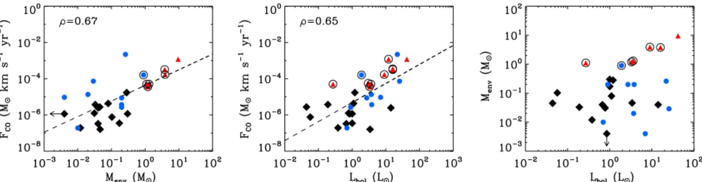
Fig. 8.Correlation plots for the outflow forceFCOusing M1, bolometric luminosityLboland the mass of the envelopeMenv. Black diamonds are from this study, red triangles from CB92, and blue circles fromHogerheijde et al.(1998), whereFCOwas calculated by the same method as in this study. The Class 0 sources are encircled. Upper limits are indicated with arrows. The dashed line indicates the best fits to the combined data set.
suggesting blending of outflow emission of two separate sources. For IRS 37 and WL 3, the outflow force is not strong, but the envelope mass for both is<10 times that of Elias 33, suggesting more evolved YSOs. The outflow is however confused due to the missing data in the southeast corner. Observations with full coverage will improve the possibility to assign this outflow to either one of the sources.
The bipolar outflow activity and outflow shape of all sources classified as “Stage 1” invan Kempen et al.(2009c) do not con-tradict their classification methods. Outflows from more evolved Stage 2 sources are in general less bipolar and more wide-angled (Arce & Sargent 2006) than Stage 1, but the opening angle can-not be derived from our CO maps due to insufficient spatial res-olution and low inclination. The difference between Stage 1 and Stage 2 can therefore not be confirmed by an outflow study, since Stage 2 sources may also show outflow activity, for example IRS 46 (in this study), IRS 48 and IRS 51 (Bontemps et al. 1996) and WL 10 (Sekimoto et al. 1997). No statistics are known for the occurrence of outflows with Stage 2 sources, but a nonde-tection would have been surprising for a Stage 1 source since all embedded protostars are expected to go through an outflow phase (Fukui et al. 1993;Arce & Sargent 2006).
When comparing the outflow forces derived in this paper with values in previous studies, significant differences are found, up to almost two orders of magnitude (see App.B). These dif-ferences can be explained to within a factor of a few by a de-tailed look into the methods and assumptions used previously. Since uncertainties in opacity and inclination potentially cause the largest variations in the outflow force, it is essential to derive these properties as accurately as possible.
Since the jet driving the outflow is assumed to originate from the spinning up of the magnetic field by the rotating disk, the outflow direction is perpendicular to the disk (Matsumoto & Tomisaka 2004). Therefore, the morphology of outflow and disk observations can be directly compared. In the last decade, very high spatial resolution observations revealing the disk structure of early phase YSOs have become available (Brinch et al. 2007; Lommen et al. 2008;Jørgensen et al. 2009) to which we compare the outflow results of this study.
The outflow of IRS 63 matches well with a disk inclination of 30◦ and north-south orientation as was found with interfer-ometric HCO+ J = 3–2 observations (Lommen et al. 2008; Jørgensen et al. 2009). The outflow of IRS 46, which is in the plane of the sky, is also consistent with an edge-on disk, as was determined by fitting a disk model to the SED (Lahuis et al. 2006). In contrast, the outflow of Elias 29 is inconsistent with the interpretation of the HCO+ velocity gradient of Lommen et al.(2008) andJørgensen et al.(2009), who argued that the
blue-shifted and red-shifted emission are indicative of a disk (i= 30◦) in the north-northwest, south-southeast direction (see Jørgensen et al. 2009, Fig. 5). As this direction is parallel to the outflow emission, it is more likely that HCO+ is instead trac-ing the dense swept-up outflow material, indicattrac-ing a small jet very close to the source. IRS 43 was interpreted as a nearly edge-on disk (i ∼90◦) in west-northwest, east-southeast direc-tion (Jørgensen et al. 2009), further supported by the elongated structure of continuum, HCO+and HCN emission, the direction of nearby Herbig Haro objects (Grosso et al. 2001) and the pro-posed radio thermal jet (Girart et al. 2000). However, this does not fit at all with the outflow result of a nearly pole-on outflow (i ∼ 10◦); the outflow with an edge-on disk would be highly inclined and therefore not even visible because the projected ve-locity is too low. As both the disk material and the swept-up outflow material are clearly observed, the configuration may be more complex. It is possible that the disk and surrounding en-velope are misaligned, similar to the L1489 IRS system (Brinch et al. 2007), as IRS 43 is a close near infrared binary with a sep-aration of 0.6 (Duchêne et al. 2007;Herczeg et al. 2011). In that case, the HCO+emission would trace the inner circumbi-nary envelope, but not the actual disk. The Herbig Haro objects that are associated with IRS 43 byGrosso et al.(2001) are also consistent with the outflow direction of IRS 44, to the north of IRS 43 (seeJørgensen et al. 2009, Fig. B1).
5.2. Trends and evolution
In order to gain a better understanding of the outflow driving mechanism, two main trends are explored: the outflow force versus the mass of the envelope and the outflow force versus the bolometric luminosity, using the outflow force results from the max (M1) method. The envelope mass is considered an evolutionary parameter, whereas the bolometric luminosity for Class 0/I YSOs is dominated by accretion luminosity (Bontemps et al. 1996).
The correlation plots are shown in Fig.8, where data from this study are combined with data from two other outflow stud-ies, which used the same method (M1) for deriving the out-flow force, i.e., CB92 (sample of mostly Class 0 sources) and Hogerheijde et al. (1998) (mostly Class I sources in Taurus). From the CB92 sample we have only included the low-mass sources. T Tau and L1551-IRS5 appear in both CB92 and Hogerheijde et al.(1998), we have chosen to include only the latter (the values forFCOare within a factor of 2 of each other).
These sources are marked accordingly in the plot.Hogerheijde et al.(1998) and CB92 measured the opacity of the line wings from13CO observations and corrected for this when determining
the outflow mass.
The well-known relationship between envelope mass and outflow force (Cabrit & Bertout 1992; Bontemps et al. 1996; Hogerheijde et al. 1998;Hatchell et al. 2007) is further extended with the results of this study. Envelope masses for our sample (see Table1) were taken fromKristensen et al. (2012) where available, otherwise fromvan Kempen et al.(2009c). The val-ues fromKristensen et al.(2012) are a better estimate due to full modeling of the SED using DUSTY, whereas the envelope masses fromvan Kempen et al.(2009c) were determined using a conversion with a single 850μm flux. Envelope masses and clas-sification for the CB92 and Hogerheijde sample were updated with more recent values, see TableE.1. The best fit through all data points is log (FCO)=(−4.4±0.2)+(0.86±0.19) log (Menv)
with Pearson’s correlation coefficientρFCO,Menv =0.67. The rela-tionship agrees within errors with the large range trend found by Bontemps et al.(1996). The data points from this study are offset from the other two studies, which may be due to the data used for deriving the envelope mass: the envelope masses in this study, except for Elias 29 and IRS 63, were derived from SCUBA 850μm emission (van Kempen et al. 2009c), whileHogerheijde et al.(1998) based their envelope mass on 1.3 mm emission. The correlation coefficient is the same as was found by Bontemps et al. (1996), who uses the annulus method (M6) and a con-stant inclination correction, confirming our previous statement that the choice of method introduces small scatter in the val-ues for the outflow force, but no significant changes over a large range. The decline of outflow force with envelope mass may re-flect a decrease of the outflow force with evolution (Bontemps et al. 1996;Saraceno et al. 1996), but since the current envelope mass reflects both age and initial core mass, the range of enve-lope masses in this sample could also represent different initial conditions (Hatchell et al. 2007), so the link with evolution is less obvious.
A second well-known relationship is between outflow force and bolometric luminosity, given in the middle panel of Fig.8. Bolometric luminosities for our sample (see Table1) were taken fromKristensen et al. (2012) where available, otherwise from van Kempen et al.(2009c). The values from Kristensen et al. are better constrained due to the inclusion ofHerschel PACS far-infrared data. The best fit through the combined data points is log (FCO)=(−5.3±0.2)+(1.1±0.2) log (Lbol) withρFCO,Lbol = 0.65. The correlation with luminosity is usually interpreted as evidence that the driving mechanism for molecular outflows is directly related to the accretion process, since the bolometric lu-minosity of low-mass YSOs is thought to be dominated by ac-cretion luminosity (Lada 1985;Yorke et al. 1995). It is widely thought that outflows are momentum-driven by a jet or wind originating from the inner disk or protostar (Bontemps et al. 1996;Downes & Cabrit 2007). The most plausible energy source for this jet or wind is the gravitational energy released by ac-cretion onto the protostar (Bontemps et al. 1996). Accordingly, the outflow force is directly related to the accretion rate ˙Macc.
Bontemps et al. (1996) found a decline of outflow force be-tween Class 0 and Class I, which has been taken as evidence that outflow force declines with age. In our combined sample the Class 0 sources are also offset from the Class I sources and fitting these two classes separately results in a significant change in offset (−5.6 vs.−4.2,±0.2 for Class I vs. 0). However, due to the selection of the older samples (the brightest outflow sources available) and the differences in data quality and derivation of
parameters, the combined sample is probably not representative of the general properties of Class 0 and Class I sources.
The envelope mass as function of bolometric luminosity has been considered as an evolutionary diagram (Saraceno et al. 1996) since the parameters are correlated, butBontemps et al. (1996) concluded that Class 0 sources do not follow the corre-lation and the diagram can only show the range of evolution-ary stages of the sample. For our sample these two parameters only have aρMenv,Lbol of 0.34 in combination with other studies (see right panel of Fig. 8) so their correlations with FCO are
independent. The similar correlation coefficients for these two relations have 3σconfidentiality levels considering the sample size (Marseille et al. 2010) so we consider the correlations to be strong.
In summary, the correlation plots agree well with previous studies of the outflow force, but a decline in evolution between Class 0 and I objects is neither confirmed or ruled out.
5.3. Outflow direction
For the L1688 part of Ophiuchus, we compare the outflow direc-tions for the different sources using Fig.1. Since these sources are clustered together, they may have experienced the same trig-ger from the same direction for the core or filament formation and the following star formation. For L1688, the orientation can be divided in three groups: IRAS 16253–2429, IRS 54, IRS 37, WL 6, IRS 44 and IRS 46 are all oriented in a northeast, south-west direction. We may even add U3 (near IRS 37) and U5 (near IRS 44) to this sample, which are well enough covered to derive their orientation. The second group contains the sources with a northwest, southeast direction: Elias 29, Elias 33, VLA 1623, WL 12 and WL 17. LFAM 26 and IRS 43 do not belong to either group. The direction of the first group agrees with the results of Anathpindika & Whitworth(2008), who concluded that the out-flow direction is perpendicular to the filament direction in 72% of cases. The implication is that angular momentum is delivered to a core forming in a filament, since the angular momentum will eventually drive the outflow. The Ophiuchus ridge in the south is indeed perpendicular to the outflow direction of the first group. A detailed study of filament velocities, such as performed for L1517 (Hacar & Tafalla 2011) suggesting core formation in two steps, could provide a better understanding of this phenomenon. The distribution of outflows over two groups with an approx-imately equal direction suggests that there have been two rate triggering events causing the star formation or two sepa-rate filaments. Considering the high values forLbolandMenvfor
the second, northern group compared to the first, southern group (mean of 3.9Land 0.36Mversus 0.6Land 0.044M) these two groups may have started star formation at different times, due to different events. This is consistent with the observation of Zhang & Wang(2009) that the star formation in Ophiuchus first took place in the denser northwestern L1689 region. It is further consistent with the suggestion that star formation in Ophiuchus was triggered by ionization fronts and winds from the Upper Scorpius OB association, located to the west of the Ophiuchus cloud (Blaauw 1991;Preibisch & Zinnecker 1999;Nutter et al. 2006).
6. Conclusions
maps and compared various analysis methods for the outflow force and assumptions that go into the calculation. The main re-sults of this study are the following:
1. All embedded sources classified as “Stage 1” byvan Kempen et al.(2009c) show bipolar outflow activity, except for those that are so close to another source that their outflows are fused. Five new outflows are detected. These results are con-sistent with the fact that every embedded source likely has a bipolar outflow. The methods used for determining inte-gration limits and deriving physical properties strongly in-fluence the results of outflow studies, but for large data sets over broad ranges ofLbol andMenvthe trends are still
simi-lar. For weak outflows and clustered star formation, detailed analysis and high-resolution observations are crucial. 2. Seven different analysis methods for deriving the outflow
force are analytically described and applied to all Ophiuchus sources in the sample, plus the well-studied sources HH 46 and NGC 1333 IRAS4A. All methods agree with each other within a factor 6. The methods that do not involve inclination correction factors give lower values for the outflow force for the largest inclination angle by a factor 2–3, but no other sys-tematic effects related to inclination exist. Although the true outflow force remains unknown, the separation method (sep-arate calculation of dynamical time and momentum) is least affected by the uncertain observational parameters.
3. The effect of subtraction of an off-source spectrum, repre-sentative of an envelope profile, is studied. After this sub-traction, the outflow material at ambient velocities, blended in with the envelope material can be measured. It is found that including ambient material does not increase the out-flow force by more than a factor of 5 and generally much less.
4. The outflow force remains constant as a function of radius, so the outflow force can be analyzed with partial coverage CO maps as long as it is centered on the source position. 5. Observational properties and choices in the analysis
proce-dure can individually affect the outflow force up to a factor of a few. The most important factor to consider is the S/N of the data: a strong dependence of the outflow force on the noise level means that the methods described cannot always be applied directly.
6. When combining the results from different studies, using dif-ferent methods, assumptions and/or data quality, scatter up to a factor of 5 can be expected. Discrepancies in derived outflow force between different studies are up to an order of magnitude and can be explained by comparing the analysis methods.
7. Comparing the outflow observations for three sources with recently obtained disk studies (Jørgensen et al. 2009) leads to revision of these disk structures. IRS 63 shows an excellent agreement for the disk orientation (perpendicular to the out-flow direction), but for Elias 29 the assumed disk emission most likely originates from the outflow material itself, close to the source, consistent with a nondetection in millimetre continuum at long baselines. IRS 43 is even more complex: the outflow direction was found to be pole-on, which is com-pletely inconsistent with the previously identified edge-on disk orientation.
8. The well-known correlations of outflow force with envelope mass and bolometric luminosity are extended with the re-sults of this study, confirming a direct correlation of outflow strength with both properties.
9. The outflows in the L1688 region can be divided into two groups, based on preferred outflow direction and signifi-cantly different evolutionary properties. This suggests a sce-nario with star formation in two separately triggered events, starting in the northwest, supporting conclusions from previ-ous work, e.g.Zhang & Wang(2009).
For further outflow studies, it is important to consider the choice of methods and assumptions that go into the calculations, espe-cially when comparing with previous results. For Ophiuchus, a complete map of the entire L1688 region in low-JCO lines, as recently performed for Perseus (Curtis et al. 2010), would pro-vide a more complete view of outflow activity, both for known as well as for new sources (such as the Us) and a more complete view of outflows from Stage 2 sources. Furthermore, the enve-lope surrounding IRS 43 should be explored in very high spatial resolution in order to understand the complex velocity structure. Limitations by single dish observations will be solved further using the Atacama Large Millimeter Array (ALMA).
Acknowledgements. The authors would like to thank Sylvie Cabrit and Mario Tafalla for useful discussions, Antonio Chrysostomou who carried out part of the12CO observations and Rowin Meijerink and Edo Loenen who carried out the 13CO observations. TheJames Clerk MaxwellTelescope is operated by the Joint Astronomy Centre on behalf of the Science and Technology Facilities Council of the United Kingdom, the Netherlands Organisation for Scientific Research, and the National Research Council of Canada. Astrochemistry in Leiden is supported by the Netherlands Research School for Astronomy (NOVA), by a Spinoza grant and grant 614.001.008 from the Netherlands Organisation for Scientific Research (NWO).
References
Anathpindika, S., & Whitworth, A. P. 2008, A&A, 487, 605 Andre, P., Ward-Thompson, D., & Barsony, M. 1993, ApJ, 406, 122 Arce, H. G., & Sargent, A. I. 2006, ApJ, 646, 1070
Bachiller, R. 1996, ARA&A, 34, 111
Bachiller, R., & Tafalla, M. 1999, in The Origin of Stars and Planetary Systems, eds. C. J. Lada, & N. D. Kylafis, NATO ASIC Proc., 540, 227
Blaauw, A. 1991, in NATO ASIC Proc. 342: The Physics of Star Formation and Early Stellar Evolution, eds. C. J. Lada, & N. D. Kylafis, 125
Bontemps, S., Andre, P., Terebey, S., & Cabrit, S. 1996, A&A, 311, 858 Bontemps, S., André, P., Könyves, V., et al. 2010, A&A, 518, L85
Boogert, A. C. A., Hogerheijde, M. R., Ceccarelli, C., et al. 2002, ApJ, 570, 708 Brinch, C., Crapsi, A., Jørgensen, J. K., Hogerheijde, M. R., & Hill, T. 2007,
A&A, 475, 915
Buckle, J. V., Hills, R. E., Smith, H., et al. 2009, MNRAS, 399, 1026
Bussmann, R. S., Wong, T. W., Hedden, A. S., Kulesa, C. A., & Walker, C. K. 2007, ApJ, 657, L33
Cabrit, S., & Bertout, C. 1990, ApJ, 348, 530 Cabrit, S., & Bertout, C. 1992, A&A, 261, 274 (CB92)
Ceccarelli, C., Boogert, A. C. A., Tielens, A. G. G. M., et al. 2002, A&A, 395, 863
Curtis, E. I., Richer, J. S., Swift, J. J., & Williams, J. P. 2010, MNRAS, 408, 1516
Dent, W. R. F., Matthews, H. E., & Walther, D. M. 1995, MNRAS, 277, 193 Di Francesco, J., Johnstone, D., Kirk, H., MacKenzie, T., & Ledwosinska, E.
2008, ApJS, 175, 277
Downes, T. P., & Cabrit, S. 2007, A&A, 471, 873 (DC07) Duchêne, G., Bontemps, S., Bouvier, J., et al. 2007, A&A, 476, 229 Evans, N. J., Dunham, M. M., Jørgensen, J. K., et al. 2009, ApJS, 181, 321 Frerking, M. A., Langer, W. D., & Wilson, R. W. 1982, ApJ, 262, 590 Fukui, Y., Iwata, T., Mizuno, A., Bally, J., & Lane, A. 1993, in Protostars and
Planets III, 603
Girart, J. M., Rodríguez, L. F., & Curiel, S. 2000, ApJ, 544, L153
Goldsmith, P. F., Snell, R. L., Hemeon-Heyer, M., & Langer, W. D. 1984, ApJ, 286, 599
Greene, T. P., Wilking, B. A., Andre, P., Young, E. T., & Lada, C. J. 1994, ApJ, 434, 614
Grosso, N., Alves, J., Neuhäuser, R., & Montmerle, T. 2001, A&A, 380, L1 Gurney, M., Plume, R., & Johnstone, D. 2008, PASP, 120, 1193
Hacar, A., & Tafalla, M. 2011, A&A, 533, A34
Herczeg, G. J., Brown, J. M., van Dishoeck, E. F., & Pontoppidan, K. M. 2011, A&A, 533, A112
Hogerheijde, M. R., van Dishoeck, E. F., Blake, G. A., & van Langevelde, H. J. 1998, ApJ, 502, 315
Johnstone, D., Wilson, C. D., Moriarty-Schieven, G., et al. 2000, ApJ, 545, 327 Jørgensen, J. K., Johnstone, D., Kirk, H., et al. 2008, ApJ, 683, 822
Jørgensen, J. K., van Dishoeck, E. F., Visser, R., et al. 2009, A&A, 507, 861 Kamazaki, T., Saito, M., Hirano, N., & Kawabe, R. 2001, ApJ, 548, 278 Kamazaki, T., Saito, M., Hirano, N., Umemoto, T., & Kawabe, R. 2003, ApJ,
584, 357
Kauffmann, J., Bertoldi, F., Bourke, T. L., Evans, II, N. J., & Lee, C. W. 2008, A&A, 487, 993
Kristensen, L. E., van Dishoeck, E. F., Bergin, E. A., et al. 2012, A&A, 542, A8 Lada, C. J. 1985, ARA&A, 23, 267
Lada, C. J., & Fich, M. 1996, ApJ, 459, 638 Lada, C. J., & Wilking, B. A. 1984, ApJ, 287, 610
Lahuis, F., van Dishoeck, E. F., Boogert, A. C. A., et al. 2006, ApJ, 636, L145 Loinard, L., Torres, R. M., Mioduszewski, A. J., & Rodríguez, L. F. 2008, ApJ,
675, L29
Lommen, D., Jørgensen, J. K., van Dishoeck, E. F., & Crapsi, A. 2008, A&A, 481, 141
Marseille, M. G., van der Tak, F. F. S., Herpin, F., & Jacq, T. 2010, A&A, 522, A40
Matsumoto, T., & Tomisaka, K. 2004, ApJ, 616, 266
Nakamura, F., Kamada, Y., Kamazaki, T., et al. 2011, ApJ, 726, 46 Nutter, D., Ward-Thompson, D., & André, P. 2006, MNRAS, 368, 1833 Preibisch, T., & Zinnecker, H. 1999, AJ, 117, 2381
Richer, J. S., Shepherd, D. S., Cabrit, S., Bachiller, R., & Churchwell, E. 2000, Protostars and Planets IV, 867
Saraceno, P., Andre, P., Ceccarelli, C., Griffin, M., & Molinari, S. 1996, A&A, 309, 827
Sekimoto, Y., Tatematsu, K., Umemoto, T., et al. 1997, ApJ, 489, L63 van Dishoeck, E. F., Kristensen, L. E., Benz, A. O., et al. 2011, PASP, 123, 138 van Kempen, T. A., van Dishoeck, E. F., Güsten, R., et al. 2009a, A&A, 501, 633 van Kempen, T. A., van Dishoeck, E. F., Hogerheijde, M. R., & Güsten, R.
2009b, A&A, 508, 259
van Kempen, T. A., van Dishoeck, E. F., Salter, D. M., et al. 2009c, A&A, 498, 167
Vladilo, G., Centurion, M., & Cassola, C. 1993, A&A, 273, 239
Wilking, B. A., Gagné, M., & Allen, L. E. 2008, Star Formation in theρOphiuchi Molecular Cloud, ed. B. Reipurth, 351
Yıldız, U. A., Kristensen, L. E., van Dishoeck, E. F., et al. 2012, A&A, 542, A86
Yorke, H. W., Bodenheimer, P., & Laughlin, G. 1995, ApJ, 443, 199 Yu, T., & Chernin, L. M. 1997, ApJ, 479, 63
Zhang, M., & Wang, H. 2009, AJ, 138, 1830
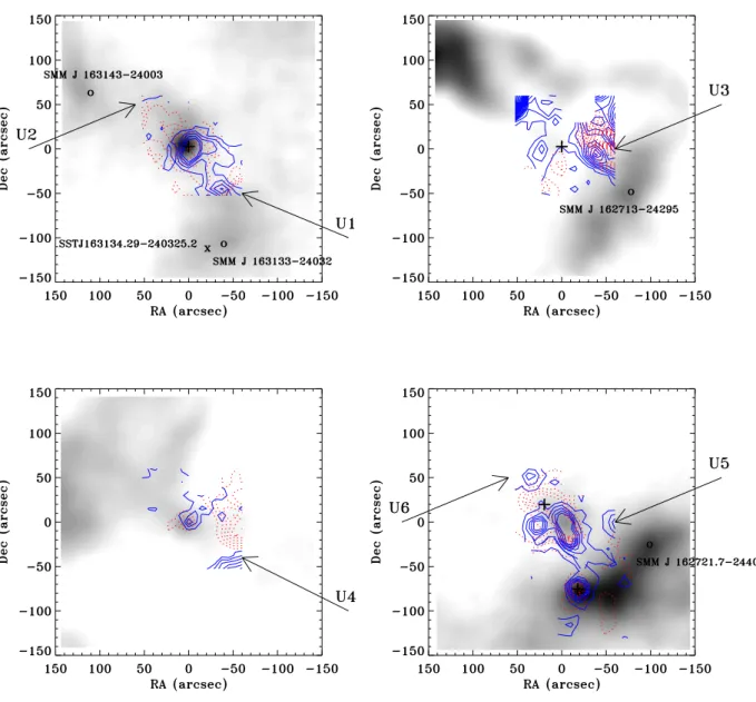
Fig. A.1.Regions around the new outflow structures (Us), showing the SCUBA 850μm emission in the background, the contour map of the integrated line wings, the sources from the sample in this study marked with pluses and the Us indicated with arrows. The nearby submillimeter cores are marked with circles and infrared sources with a cross. (Top left) The region around IRS 63. (Top right) The region around IRS 37. (Bottom left) The region around WL 12. (Bottom right) The region around IRS 44.
Appendix A: Newly discovered outflows
From detailed spectral analysis, new bipolar outflow structures were discovered in several CO maps, not belonging to any of the sources in the embedded source sample ofvan Kempen et al. (2009c). In this section we look for other suitable candidates of embedded sources. The partial coverage of these outflows ex-tends the field in which to look for a candidate.
– The outflow structure U1 southwest of IRS 63 may originate from the submillimeter core SMM J 163133–24032, which was matched byJørgensen et al.(2008) with theSpitzerYSO candidate SSTc2d J163134.29-240325.2 (Evans et al. 2009), located 24away, classified as a Class I source withLbol=
0.88LandTbol=870 K.
– For U2, selecting a candidate is somewhat difficult, as only a small piece of the red lobe is covered and therefore the direction of the originating source is unknown. The most likely candidate is the submillimeter core SMM J 163143– 24003 (Jørgensen et al. 2008) at 2.2northeast of IRS 63 (see
Fig.A.1) with a dust temperature of 15 K. No infrared source is known near this location.
– U3 is located to the west of IRS 37. The elongated struc-ture and direction of the outflow suggest that the power-ing source is located to the southwest. The large submil-limeter core SMM J162713–24295 (Jørgensen et al. 2008) is a likely candidate (see Fig.A.1) with a dust temperature of 18 K. The shape of this submillimeter core is consistent with the outflow direction, which is usually perpendicular to the ridge (Anathpindika & Whitworth 2008). Again, no in-frared source is known at this location.
– The outflow U4 is clearly visible in the WL 12 map (Fig.A.1). The center of origin is about 16:26:40,−24:35:27. There are no submillimeter cores or infrared sources nearby. Estimates of a SED orTbolare therefore not possible at this
time.