ASSESSING EXPOSURE TO CHLORINATED SOLVENTS FROM THE SUBSURFACE TO INDOOR AIR PATHWAY
Jill E. Johnston
A dissertation submitted to the faculty of the University of North Carolina at Chapel Hill in partial fulfillment of the requirements for the degree of Doctor of Philosophy in the
Department of Environmental Sciences and Engineering.
Chapel Hill 2013
Approved by:
Jacqueline MacDonald-Gibson Richard (Pete) Andrews Joachim Pleil
ABSTRACT
JILL E. JOHNSTON: Assessing Exposure Of Chlorinated Solvents from the Subsurface to Indoor Air Pathway
(Under the direction of Jacqueline MacDonald Gibson)
The migration of chlorinated volatile organic compounds from groundwater to indoor air—known as vapor intrusion—is an important exposure pathway at sites with contaminated groundwater. However, monitoring indoor air quality in the hundreds or thousands of at-risk homes at each site is logistically and financially infeasible. Screening methods are needed to prioritize homes for monitoring and remediation. Current
screening approaches do not adequately account for the substantial spatial and temporal variability in vapor intrusion risk, in part because the causes of this variability are not well understood. This work explores variability in vapor intrusion risk in a case-study community and then develops two different modeling approaches for screening at-risk homes.
We employed a community-based approach to collect indoor air samples and analyze vapor intrusion risk in 20 homes at a case-study site. Results demonstrate that indoor concentrations of tetrachloroethylene from vapor intrusion vary by an order of magnitude across space and time. We show that key factors affecting this variability include barometric pressure drop, humidity, wind speed, and season.
Using data collected from 370 homes in the National Database on Vapor
unmonitored homes. The resulting predictions decrease the rate of false negatives compared with the U.S. Environmental Protection Agency’s (EPA) current screening approach, which assumes that indoor air concentration will not exceed 1/1,000 times the soil gas concentration just above the groundwater.
Finally, we demonstrate a second approach for improving the accuracy of screening by using Bayesian statistical techniques to integrate observational data into a mechanistic model describing the physical and chemical processes driving vapor intrusion. The resulting calibrated model also decreases the rate of false negatives in screening homes for vapor intrusion risks when compared with the current EPA approach.
ACKNOWLEDGEMENTS
I am grateful to my advisor, Jackie MacDonald Gibson, for her guidance, advice, and mentorship.
To the membership of my committee, thank you for your support along the way and for providing useful insights and suggestions that enhanced this work.
I am forever grateful to the good people of the Southwest Workers Union and the Committee for Environmental Justice Action for your inspiration, leadership and courage.
I thank the National Science Foundation for its support through a graduate research fellowship. And to Harry O’Neill and the other individuals at Beacon Environmental Services, I appreciate your mentorship and help in data collection and analysis.
PREFACE
TABLE OF CONTENTS
LIST OF TABLES ...x
LIST OF FIGURES ... xi
LIST OF ABBREVIATIONS ... xiii
LIST OF SYMBOLS ... xv
CHAPTERS 1. Introduction ... 1
1.1. Overview of this Research ...1
1.2. Scope of Vapor Intrusion Problem and Potential Health Issues ...3
1.3. Vapor Intrusion Exposure Pathway: Monitoring Considerations ...5
1.4. Vapor Intrusion Exposure Pathway: Modeling Approaches ...6
1.5. Vapor Intrusion Regulations and Policy Approaches ...9
1.6. Study Site ...15
1.7. Motivation and Objectives ...17
2. Spatiotemporal Variability of Tetrachloroethylene in Residential Indoor Air Due to Vapor Intrusion: A Longitudinal, Community-Based Study ... 19
2.1. Introduction ...19
2.2. Materials and Methods ...25
2.3. Results ...33
2.4. Discussion ...39
3. Screening Houses for Vapor Intrusion Risks: A Multiple Regression
Analysis Approach ... 43
3.1. Introduction ...43
3.2. Methods...47
3.3. Results and Discussion ...52
3.4. Conclusions ...65
4. Updating Exposure Models of Indoor Air Pollution Due to Vapor Intrusion: Bayesian Calibration of the Johnson-Ettinger Model ... 66
4.1. Introduction ...66
4.2. Methods...70
4.3. Results and Discussion ...80
4.4. Conclusions ...92
5. Concluding Remarks ... 94
5.1. Overview of Policy Issues and Current Research Limitations ...94
5.2. Key Findings and Implications ...97
5.3. Future Research Needs ...104
5.4. Conclusions ...111
APPENDIX A. Spatiotemporal Variability of Tetrachloroethylene in Residential Indoor Air Due to Vapor Intrusion: A Longitudinal, Community-Based Study – Supplementary Material………..112
APPENDIX B. Screening Houses for Vapor Intrusion Risks: A Multiple Regression Analysis Approach – Supplementary Material……...……….114
APPENDIX C. Updating Exposure Models of Indoor Air Pollution Due to Vapor Intrusion: Bayesian Calibration of the Johnson-Ettinger Model – Supplementary Material………...…...………..118
LIST OF TABLES
Table 2.1. Characteristics of the 20 homes included in this study………34 Table 2.2. Summary statistics for the key continuous variables included in the
regression model..………35
Table 2.3. Average marginal effects for the within-home variability of natural
log PCE indoor air concentration (ln-µg/m3) due to vapor intrusion....……..37
Table 2.4. Population-averaged effects of model covariates on between-home
(spatial) variability of natural log PCE indoor air concentration (ln-µg/m3) due to vapor intrusion……….………...38
Table 3.1. Summary statistics for the key continuous variables included in
the regression model….………...54
Table 3.2. Effects of model covariates on variation in the log groundwater
vapor intrusion attenuation factor………..………..55
Table 3.3. Comparison of three methods for predicting groundwater attenuation
factors to measured factors.……….63
Table 4.1. Complete set of equation needed to implement the Johnson-Ettinger
model………...73
Table 4.2. Basic properties of houses and measured concentration of PCE
indoors……….…75
Table 4.3. Prior and MCMC posterior estimates of the mean values and standard
deviations of the model parameters……….83
Table 4.4. Comparing model performance of the deterministic approach, the
prior predictions and the two updated model predictions to the
measured indoor air concentrations……….87
Table A.1. Analysis of variance of covariates considered in the model……….113 Table B.1. Proportion of the variation of log vapor intrusion attenuation factor
for residential homes explained by environmental, household and
multilevel factors………..…...….….117
LIST OF FIGURES
Figure 1.1. Summary of the physical processes that influence the vapor intrusion
pathway………7
Figure 1.2. Conceptual framework of Johnson-Ettinger model……….….8 Figure 1.3. Schematic summary of EPA’s approach to vapor intrusion sites,
based on 2002 draft guidance……….11
Figure 1.4. Measured groundwater vapor attenuation factors compared to
the indoor air concentrations shown on a log scale for observations included in the EPA National Vapor Intrusion Database………...13
Figure 1.5. Map of Kelly Air Force Base and the adjacent contaminated
groundwater plume……….16
Figure 2.1. Summary of EPA’s previous subslab, crawl space, and indoor air
measurements for PCE………...24
Figure 2.2. Map showing the approximate location of the 20 homes sampled
and the PCE concentrations in the underlying groundwater plume………...25
Figure 2.3. Example data collection schedule per house………..28 Figure 2.4. Indoor air concentration of PCE by study home.………...35 Figure 2.5. Temporal variation in indoor PCE concentrations in homes
with at least one sample above the detection limit………....…….36
Figure 3.1. Schematic of nested multilevel model………51 Figure 3.2. Predicted (natural log) vapor intrusion attenuation factor based
on multilevel model for PCE, assuming mean groundwater region and site-level characteristics for various combinations of groundwater depth (m), soil type, foundation type, and season………58
Figure 3.3. Comparison of the log mean predictions (blue) and 95th percentile
predictions (orange) with the actual log of the attenuation
factor………..61
Figure 4.1. Sketch of model framework for the Bayesian calibration
methodology………..71
Figure 4.2. Comparison of the measured indoor air PCE concentrations due
to vapor intrusion and EPA-recommended deterministic
Figure 4.3. Box plots of the prior and posterior distributions (Model 1 and
Model 2) for each of the four household parameters and five soil parameters (for clay and SiC: silty clay soil) calibrated during the Bayesian updating……….84
Figure 4.4. Measured predictions versus updated model predictions. The
dotted gray horizontal line represents the PCE detection limit
(0.13 µg/m3)………86
Figure 4.5. Sensitivity analysis of uncertain variables. The soil parameters
displayed are for the silty clay (SiC) soil type………...90
Figure A.1. An example of the passive sampling set up used in residential
homes in this study………..….113
Figure B.1. Distribution of pooled vapor intrusion attenuation factors for all
observations included in statistical analysis………...………..114
Figure B.2. Distribution of measured natural logarithm of attenuation factors
for CVOCs across the sites and groundwater regions; black line tracks the mean attenuation factor at each site and region and shows site-to-site and region-to-region variability……….…………..115
Figure C.1. Estimated PCE groundwater concentrations (µg/L) in 2011………...……119
Figure C.2. Estimated groundwater levels (m below surface) in 2011…………...…..119 Figure C.3. Measured values (circle- mean with 90% confidence interval)
compared to the prior probability predictions (x-mean with 90% confidence interval)………..120
LIST OF ABBREVIATIONS AC air conditioning
AIC Akaike information criterion
AFB Air Force base
ANOVA analysis of variance
B basement
BME Bayesian maximum entropy
C clay soil
CEJA Committee for Environmental Justice Action
CL clay loam soil
CS crawl space foundation
CVOCs chlorinated volatile organic compounds
DCE dichloroethene
EPA U.S. Environmental Protection Agency
F fine-grained soil
GSD geometric standard deviation
HAPSITE Hazardous Air Pollutants on Site
HtA Houston Black clay
JEM Johnson-Ettinger model
LN lognormal
LvA Lewisville silty clay
MCMC Markov Chain Monte Carlo
OLS ordinary least squares
PCE tetrachloroethylene
RIOPA relationship of indoor, outdoor, and personal air
RMSE root mean squared error
S summer
SC sandy clay soil
SCL sandy clay loam soil
Sd standard deviation
SiC silty clay soil
TCA trichloroethane
TCE tricholorethylene
TD-GC/MS thermal desorption gas chromatograph/ mass spectrometer
USDA U.S. Department of Agriculture
VC very coarse-grained soil
VOCs volatile organic compounds
LIST OF SYMBOLS
A = building area, cm2
A
b = area of enclosed space below grade, cm 2α = alpha, vapor intrusion attenuation coefficient, unitless Cindoor = contaminant concentration in indoor air (mass/volume) Csource = contaminant source concentration (mass/volume)
D
air = chemical specific molecular diffusion coefficient in air, cm2/s DH2O = chemical specific molecular diffusion coefficient in water, cm 2/s Deff = effective diffusion coefficient, cm2/s
Dcrackeff = effective diffusion coefficient through cracks, cm2/s
Dc,zeff = effective diffusion coefficient across the capillary zone, cm2/s Dieff = effective diffusion coefficient across soil layer i, cm2/s
Dtotal eff
= total overall effective diffusion coefficient, cm2/s = indoor-outdoor pressure difference, g/cm-s2
E
b = air exchange rate (1/hr)g
= acceleration due to gravity, cm/s2 (constant)H
i = chemical specific Henry’s law constant, unitlessk
= soil permeability near foundation, cm2 /sK
i = soil intrinsic permeability, cm2KH ,i = chemical-specific Henry’s constant, unitless
K
s = soil saturated hydraulic conductivity, cm/sL
crack = enclosed space foundation or slab thickness, cmL
i = Thickness of soil layer i, cmL
t = source-building separation, cmM = van Genuchten shape parameter, unitless MH = building mixing height, cm
µ = viscosity of air, g/cm-s
µw = dynamic viscosity of water, g/cm-s (constant)
η = fraction of foundation surface area with cracks, unitless Qbuilding= building ventilation rate, cm3/s
Q
soil = volumetric flow rate of soil gas into the enclosed space, cm3/sR
crack = effective crack radius or width, cm ρw = density of water, g/cm3 (constant)S
te = effective total fluid saturation, unitless θm = volumetric moisture content, cm3/cm3 θr = residual soil water content, cm3/cm3 θT = total soil porosity, cm3/cm3V
b = building volume, cm3X
crack = total length of cracks through which soil gas vapors are flowing (i.e. perimeter),cm
CHAPTER 1
Introduction
1.1. Overview of this Research
Although a number of important pieces of environmental legislation have been enacted over the past 40 years, these regulations largely ignore the indoor sphere. No federal agency or law specifically regulates the quality of air in residential indoor environments, even though Americans spend 85-90% of their time indoors and the majority of exposure to air contaminants occurs there (Hodgson, Garbesi, Sextro, & Daisey, 1992; Klepeis et al., 2001; Spengler & Sexton, 1983). Compared to the
consumption of drinking water, humans inhale 10,000 times more liters of air per day, an involuntary exposure that is very difficult to replace (Schuver, 2007). Over the past decade, vapor intrusion has been recognized as a possible significant health hazard to residents living near toxic sites and polluting facilities (Johnson & Ettinger, 1991; U.S. Environmental Protection Agency, 1992). Despite this evidence and growing interest in this exposure pathway, there has not been a systematic approach to exposure assessment or the development of appropriate, evidence-based policy to indoor air pollution due to vapor intrusion.
soil) as well as private space (the interior of private buildings). At vapor intrusion sites, exposure is both inescapable and involuntary (Fitzgerald, 2009). Current regulatory guidance is limited in scope, and robust decision-making tools for managing vapor intrusion risks are lacking. The subsequent chapters of this dissertation evaluate the variability and uncertainty of the vapor intrusion pathway in order to inform the
regulatory framework around the collection of measurements and the use of quantitative screening and modeling tools in the evaluation of exposure. The research focuses on an understudied region in the United States—the South—to examine the mechanisms and forces at work in a southern climate. This study compares data from measurements and modeling efforts and quantifies the uncertainty of measuring and predicting indoor air concentrations. The knowledge gained may be useful in creating and refining models to better predict exposure due to vapor intrusion and to support the development of
quantitative decision-making tools useful in the assessment of contaminated sites. The research is structured around three objectives:
• Objective 1: Characterize spatial and temporal variability in the distribution of
tetrachloroethylene (PCE) in indoor air in residences in a case study community that overlies groundwater contaminated with these chemicals. This objective has two components: (a) determine the concentrations of PCE in the air attributable to vapor intrusion in 20 homes, and (b) evaluate the factors that influence both temporal and spatial variability in the indoor concentrations of PCE.
• Objective 2: Evaluate the current U.S. Environmental Protection Agency (EPA)
an alternative method based on a multivariate analysis of the vapor intrusion database.
• Objective 3: Demonstrate a novel approach to the integration of a mechanistic
model with stochastic techniques in order to improve characterization of exposure due to vapor intrusion in a contaminated community.
1.2. Scope of Vapor Intrusion Problem and Potential Health Issues
When a subsurface release of volatile chemicals (those that easily transform to gas phase) occurs near buildings, contaminants can migrate upwards and result in vapor-phase contaminant intrusion into the indoor air. A particular class of volatile chemicals, chlorinated volatile organic compounds (CVOCs), includes commonly used solvents such as tetrachloroethylene (also called perchloroethylene, or PCE). CVOCs are among the most frequently detected groundwater contaminants at hazardous waste sites in the United States (Agency for Toxic Substances and Disease Registry, 2007; McCarty, 2010). They persist in the environment and are difficult to remediate (Simpkin & Norris, 2010; Travis & Doty, 1990). A commonly accepted practice in the remediation of CVOC plumes is “monitored natural attenuation”—that is, allowing natural physical processes to dilute and biological processes to degrade the contaminants to allowable levels, an
Vapor intrusion exposures are real, direct, and chronic. The concentration of contaminants above recommended human health exposure levels in indoor air has been attributed to vapor intrusion from several sites (EerNisse, Steinmacher, Mehraban, Case, & Hanover, 2009; Folkes, Wertz, Kurtz, & Kuehster, 2009; McDonald & Wertz, 2007). Volatile organic compounds are reported at about half of known hazardous waste sites. Of these, approximately half may have conditions that favor intrusion of vapors into buildings, amounting to tens of thousands of sites nationwide (Schuver, 2007).
Levels of CVOCs in indoor air are typically five to 10 times those in ambient air (Steinemann, 2004; Wallace, 2001). Inhalation can lead to higher toxicities than
1.3. Vapor Intrusion Exposure Pathway: Monitoring Considerations
Determining when and where vapor intrusion is occurring—and subsequently remediating it—is challenging. Monitoring techniques must be able to measure minute concentrations of chemicals in air, in the realm of less than one part per billion (by volume), and chemicals of concern that volatilize from household products, including dry-cleaned clothes, must be identified and removed. Current practice requires the investigation assume a building-by-building analysis, and the evaluation techniques can be highly invasive, requiring entry by agency personnel and the placement of monitors inside private homes.
At the community scale, current knowledge of the vapor intrusion pathway derives from a few detailed case studies where indoor air concentrations were measured across space (Folkes et al., 2009; Kliest, 1989; McDonald & Wertz, 2007; Schreuder, 2006). The results have demonstrated significant spatial variability, and often the majority of the risk has been concentrated in a few homes. Further, recent research has demonstrated that concentrations attributed to vapor intrusion vary daily, weekly, and seasonally (Luo, Holton, Dahlen, & Johnson, 2011; McHugh, Nickles, & Brock, 2007; McHugh et al., 2012). Factors influencing temporal variability are a current area of investigation, with few published studies available.
In addition, indoor sampling is further complicated by the potential for
1.4. Vapor Intrusion Exposure Pathway: Modeling Approaches
Determining if and when an exposure pathway exists is further limited by
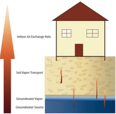
shortcomings in scientific understanding. The movement of vapors from the subsurface is dependent on multiple elements. The understanding of the transport mechanisms
Figure 1.1. Summary of the physical processes that influence the vapor intrusion
pathway.
There are two general categories of vapor intrusion models proposed: one dimensional (simplified) models and multidimensional numerical models. In general, one-dimensional models, like the Johnson-Ettinger model (JEM), are used in site evaluation to identify areas of potential highest risk and/or to determine whether further investigation of indoor air is warranted. The JEM (Figure 1.2) is widely used for
regulatory guidance on vapor intrusion in the United States and estimates the vapor attenuation ratio, α, a unitless parameter that relates the indoor air concentration to the concentration in the vapor phase at equilibrium with the contaminated groundwater:
where α is the vapor attenuation ratio, Cindoor is the contaminant concentration in indoor air (mass/volume), and Csource is the contaminant vapor-source concentration
(mass/volume).
Figure 1.2. Conceptual framework of Johnson-Ettinger model.
The JEM couples one-dimensional steady-state diffusion of volatile compounds through porous media with diffusion and advection through the building foundation in the following equation to estimate α (Johnson & Ettinger, 1991):
(2)
where Dtotaleff
enclosed space (cm3/s), Lcrack is the enclosed space foundation or slab thickness (cm), η is the fraction of foundation surface area with cracks (unitless), and Dcrack
eff
is the effective diffusion coefficient through the cracks (cm2/s). However, many of these parameters are difficult to characterize.
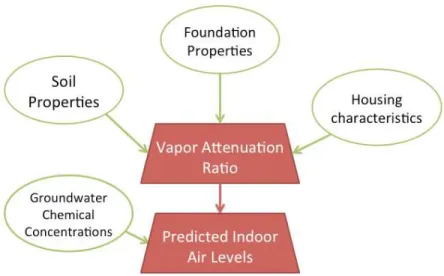
The output of the JEM is intended to serve as an estimate of the influence of groundwater contamination on indoor air and to identify areas for further testing.
Important parameters that influence vapor intrusion—and are included in the model—are soil characteristics (e.g., porosity, moisture content), building characteristics (air
exchange rate, foundation type, and volume), and pressure differentials between the indoor and subsurface environments. Comparisons between modeled and measured α values indicate that with reasonable input parameters the JEM can predict within one order of magnitude the expected actual indoor air concentrations (Hers & Zapf-Gilje, 2003).
1.5. Vapor Intrusion Regulations and Policy Approaches
In November 2002, the EPA issued draft guidance titled “OSWER Draft
Guidance for Evaluating the Vapor Intrusion to Indoor Air Pathway from Groundwater and Soils (Subsurface Vapor Intrusion Guidance),” which aimed to “provide a tool to help the ‘user’ conduct a screening evaluation as to whether or not the vapor intrusion exposure pathway is complete and, if so, whether it poses an unacceptable risk to human health” (U.S. EPA, 2002). The guidance proposes a risk-based approach for site
building-by-building) decisions at thousands of diverse sites (Daley, 2007; Sigman, 1998).
1.5.1. EPA Vapor Intrusion Assessment Tiers
Figure 1.3. Schematic summary of EPA’s approach to vapor intrusion sites, based on
2002 draft guidance.
Once a site passes the first tier, the second tier involves estimating the expected indoor air concentrations due to vapor intrusion. The 2002 guidance establishes
groundwater targets by applying a generic attenuation factor, α, to screen vapor intrusion sites for study; EPA suggests that their assumptions represent the “worst-case conditions” (U.S. EPA, 2002). The attenuation factor is the ratio between the vapor-phase
to use the indoor air concentration predictions to convert exposure into cancer risk estimates and recommend a course of action based on the risk calculation. There is no definitive action-level threshold; the EPA provides indoor air targets based on 10-4, 10-5 and 10-6 risk levels. In addition, most state-level guidance provides an action-level threshold; across the various states, these values can vary by three orders of magnitude for the various CVOCs of concern (Eklund, Beckley, Yates, & McHugh, 2012).
Once sites have been selected for further screening, the next step is to take measurements of concentrations in indoor air. The collection of indoor air samples is suggested only if a home (or site) screens into the final stage based on previous modeling. The favored EPA method is a 24-hour active sample using a summa canister. This
technique actively pumps air through the canister to capture a specified volume. This single sample is considered to be a representative concentration upon which to base an action decision.
1.5.2. Limitations of Current Regulatory Approach
found to produce the least conservative predictions (Provoost et al., 2009). The use of the JEM as a screening tool has been cautioned against because of the potential for false negatives and the frequency of underpredictions (Provoost et al., 2010). Complex three-dimensional models have been proposed and may be more accurate for an individual home, but these approaches are not scalable to a community level and require numerous detailed inputs (Bozkurt, Pennell, & Suuberg, 2009; Pennell, Bozkurt, & Suuberg, 2009; Yao, Shen, Pennell, & Suuberg, 2011; Yao & Suuberg, 2013). Few studies have
compared modeling results to data, but in most cases the various models are unable to adequately explain the observations (Yao, Shen, Pennell, & Suuberg, 2013).
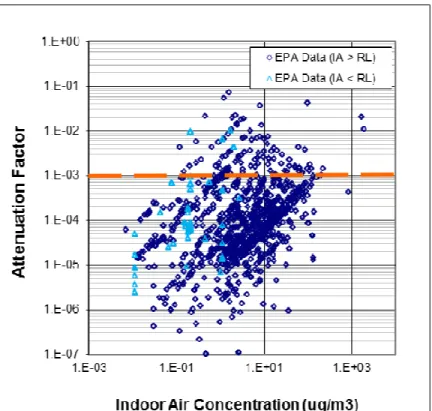
Figure 1.4. Measured groundwater vapor attenuation factors compared to the indoor air
Finally, the method of only sampling from a single point in space and time is unlikely to reflect community-scale exposure. Due to the temporal variability of the process (as well as the potential for confounding indoor sources), a single sampling event is insufficient to provide definitive information about vapor intrusion risks (McHugh et al., 2012). Residents have expressed reservations about allowing monitoring using collection devices known as summa canisters, which are invasive and costly, prone to measurement error, and require batteries or electricity (Siegel, 2009; Wang & Austin, 2006). As a result of uncertainties, an accurate analysis requires robust data sets, which carry substantial costs.
1.5.3. Status of Current Federal Guidance
Since issuing the draft guidance, the EPA has yet not finalized the document. Separately, 29 states, stakeholder groups, and other federal agencies (including the Department of Defense, Department of Energy, and Department of Housing and Urban Development) have issued vapor intrusion guidance or other related technical documents, which vary widely in approach and scope (Fitzgerald, 2009; McAlary & Johnson, 2009; Simon, 2011). The Office of the Inspector General issued a report critical of the EPA’s inadequate response and the incomplete scope of the 2002 guidance (U.S. EPA, 2009). The EPA has blamed the lack of progress toward finalizing guidance or developing regulations on both administrative and scientific barriers (U.S. EPA, 2009). The EPA was scheduled to release a final draft of the 2002 guidance in December 2012, but the
this research focuses on the tools proposed (or used) by environmental agencies to
determine whether vapor intrusion is occurring and if a site requires monitoring or further remedial action.
1.6. Study Site
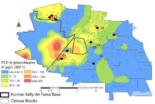
For much of this research, I used a case study site of a low-income neighborhood adjacent to the former Kelly Air Force Base (Figure 1.5), which operated in the southwest side of San Antonio, Texas, for nearly 85 years, serving as a logistic headquarters for the U.S. Air Force. Over that time period, the activities and practices at the base
Figure 1.5. Map of Kelly Air Force Base and the adjacent contaminated groundwater
plume.
1.7. Motivation and Objectives
In summary, a key unresolved debate is what constitutes sufficient evidence of a complete vapor intrusion pathway and how to identify whether vapor intrusion exposure may be occurring in individual houses (U.S. EPA, 2009). Ultimately, the vapor intrusion pathway is house-specific and prone to temporal fluctuations. However, in most cases hundreds or even thousands of buildings are potentially impacted. While it is impractical to monitor every home, it is also problematic to use over-simplistic decision-making models to determine whether additional investigation is needed. Due to the known limitations of the proposed modeling-based tools, alternative approaches should be considered in order to improve exposure estimates and provide a better estimate of health risks and remediation needs. So far, neither an adequate tool to identify high-risk areas nor the ability to assess the exposure at a community-wide level exists.
The overarching aim of this dissertation is to investigate tools for predicting household indoor air contamination due to the migration of CVOCs from the subsurface and to assess decision-making tools used to make policy choices regarding vapor
characterize the uncertainty and variability in the risks, and inform an alternative site-specific decision-making tool.
The remainder of this dissertation is organized into four chapters. Chapter 2 describes a method to quantify spatial and temporal variability in indoor concentrations of PCE in San Antonio, as well as integrate community participation. Chapter 3 examines the limitations of the current generic screening approach based on observations from the EPA vapor intrusion database and proposes a regression-based approach for screening potential vapor intrusion sites. Chapter 4 considers stochastic techniques to improve site-level exposure estimates based on the JEM when some site-specific data has been
CHAPTER 2
Spatiotemporal Variability of Tetrachloroethylene in Residential Indoor Air Due to Vapor Intrusion:
A Longitudinal, Community-Based Study1
2.1. Introduction
Volatile organic compounds (VOCs) are often found at higher concentration indoors compared to the outdoor environment (Adgate et al., 2004; Dodson, Levy, Houseman, Spengler, & Bennett, 2009). VOCs are capable of migrating from
contaminated groundwater through overlying soil and building foundations, resulting in vapor-phase contaminant intrusion into indoor air (Environmental Quality Management, 2004; Johnson & Ettinger, 1991). Tetrachloroethylene (PCE) is among the most
frequently detected groundwater contaminants at hazardous waste sites in the United States (Agency for Toxic Substances and Disease Registry, 2007; McCarty, 2010). The inhalation of vapors inside homes is an understudied field, but prior research suggests it may be an important pathway by which communities at hazardous waste sites are exposed to chlorinated VOCs (CVOCs) in groundwater (Ferguson, Krylov, & McGrath, 1995; Fischer et al., 1996; Little, Daisey, & Nazaroff, 1992; Provoost et al., 2008). Long-term exposure to CVOCs has been linked to cancer, kidney and liver disease, and
reproductive problems such as pregnancy loss, developmental abnormalities, and
1 Johnston, J. E., & MacDonald Gibson, J. 2013, in press. Spatiotemporal variability of
birth weights (Aschengrau et al., 2009; Agency for Toxic Substances and Disease
Registry, 1997; Beliles, 2002; Doyle, Roman, Beral, & Brookes, 1997). Elevated rates of cancers, low birth weights, fetal growth restrictions, and cardiac defects have been reported at sites with CVOC vapor intrusion, although causality has not been established (Agency for Toxic Substances and Disease Registry, 2006; Colorado Department of Public Health and Environment, 2002; Forand, Lewis-Michl, & Gomez, 2011). Due to these potential health risks and the frequency of PCE detection in contaminated groundwater, the potential for PCE exposure via vapor intrusion is an important consideration when making decisions regarding groundwater remediation.
Spatial and temporal variability has been observed in subslab and indoor air concentrations of CVOCs above contaminated groundwater plumes (see, for example, Folkes, Wertz, Kurtz, & Kuehster, 2009; Luo, Holton, Dahlen, & Johnson, 2011; McDonald & Wertz, 2007; McHugh, Nickles, & Brock, 2007; Schreuder, 2006).
Variability across space and time has also been observed in indoor radon concentrations, which also result from vapor intrusion (albeit from natural geologic sources rather than anthropogenic contamination) (Davies & Forward, 1970; Groves-Kirkby, Denman, Phillips, Crockett, & Sinclair, 2010; Steck, Capistrant, Dumm, & Patton, 2004). Hence, an indoor air sample from a single point in space and time is unlikely to reflect
community-scale exposure to vapor intrusion risks. Furthermore, previous work suggests that groundwater concentrations are not adequate surrogates for measuring vapor
(Fitzpatrick & Fitzgerald, 2002; Folkes et al., 2009). In site assessments, often only a single 24-hour indoor air sample is taken from a small number of homes in an affected community, although U.S. Environmental Protection Agency (EPA) and state guidance often recommend that multiple samples be collected from a single home following a multi-tiered approach to vapor intrusion investigations (Eklund, Beckley, Yates, & McHugh, 2012; U.S. EPA, 2002). For example, in the EPA’s National Vapor Intrusion Database, the sampling frequency is as follows: a single-point-in-time sample in 84% of buildings, two samples collected in 10% of buildings, three to five samples in 5% of buildings, and more than five samples in 1% of cases. Collecting one or two samples, as is the current common practice, will not account for the potential spatial and temporal variability and may under- or overestimate the true exposure risk. An inaccurate characterization of exposure may result in inaccurate human health risk assessments.
Previous work has helped describe the mechanisms governing vapor intrusion and potential causes of variability. Pressure-driven flow is an important mechanism for gas entry into homes (Fitzpatrick & Fitzgerald, 2002; Nazaroff et al., 1985). Building underpressurization, changes in barometric pressure, wind, and diurnal fluctuations in temperature all can influence indoor-outdoor pressure differentials and hence vapor flow into homes (Adomait & Fugler, 1997; Garbesi & Sextro, 1989; McHugh et al., 2012). When these processes lead to negative building pressure (i.e., outdoor pressure greater than indoor pressure), the rate of vapor intrusion increases. However, the relationships among these factors are complex and the net effects on vapor intrusion difficult to
indoor radon concentrations has been observed (Luo, 2009; Nazaroff & Doyle, 1985; Nazaroff et al., 1985; Turk, Prill, Grimsrud, Moed, & Sextro, 1990).
Further understanding of the spatiotemporal drivers of vapor intrusion is needed in order to inform decisions about the extent of indoor air monitoring necessary to adequately estimate exposure risks in communities overlying contaminated groundwater. Yet, indoor air monitoring is intrusive, and residents can be resistant to allowing
researchers or government personnel into their homes (Siegel, 2009). Due in part to this challenge, other studies of temporal variability have focused on a single home rather than multiple homes, and studies of spatial variability have been able to collect only one or two 24-hour samples in each home.
This study addresses the need for community-wide assessment of spatiotemporal variability in vapor intrusion risks. The study, the first of its kind in the southern United States, integrated longitudinal and cross-sectional data collection at a contaminated site adjacent to the former Kelly Air Force Base in southwest San Antonio, Texas. We examined the effects of household characteristics and meteorological conditions on observed fluctuations in indoor air PCE concentrations to determine whether changes in (a) meteorological conditions, (b) soil type, (c) groundwater concentration, and (d) household characteristics significantly explain spatiotemporal variability in indoor PCE concentrations attributable to vapor intrusion. A better understanding of the drivers of temporal and spatial variability in vapor intrusion can inform decisions regarding monitoring and exposure assessment in affected communities.
extended five miles to the southeast of the base and underlie approximately 30,000 homes. The shallow groundwater lies 1 to 12 m below the homes. PCE concentrations in the groundwater range from 1 µg/L to 200 µg/L in the residential areas. Off-base
groundwater remediation began in 2004 and is ongoing.
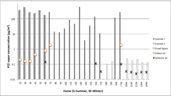
The EPA evaluated a cohort of 24 houses for vapor intrusion in May 2008 and February 2009. During the 2008 sampling, the EPA collected one or two samples beneath each home’s foundation, outdoor air samples in selected locations, and a single indoor sample in a subset of homes. The sampling protocol followed EPA method TO-15, in which 6-liter collection devices known as summa canisters (in this case with a PCE detection limit of 0.14 µg/m3) are deployed to capture an air sample later analyzed in a laboratory (U.S. EPA, 1999a). For homes in which indoor air was tested, the EPA
Figure 2.1. Summary of EPA’s previous subslab, crawl space, and indoor air
measurements for PCE.
2.2. Materials and Methods
We sampled indoor air for PCE in 20 homes over a 12-day period during summer (July-August) 2011 (Figure 2.2). We resampled nine of the homes over another 12-day period in winter (February-March) of 2012. For the winter period, we divided the homes into those with evidence of vapor intrusion (at least one detection above 0.25 µg/m3) and those without. We randomly selected six homes from those that showed evidence of vapor intrusion and an additional three from the homes with no detectable PCE.
Figure 2.2. Map showing the approximate location of the 20 homes sampled (ovals,
black ovals for homes sampled in winter) and the PCE concentrations in the underlying groundwater plume.
2.2.1. Indoor Air Sources Identification
additional PCE sources during the mid-study resampling. In 18 of the homes, residents had a detached storage shed or garage, while two homes had no garage. These detached structures were neither evaluated nor included in the analysis.
2.2.2. Indoor Air Sampling
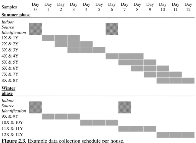
During the summer sampling event, we collected a total of eight duplicate samples (16 total samples) over a period of 12 days in each of the 20 study homes. For the second sampling period, four sample pairs per home were collected sequentially over a 12-day period in February and March. A total of 392 samples were collected (186 paired measurements). Passive monitoring devices were shipped to the field site, and duplicate field blanks were included in each sampling season. In each case, samplers were left in place for three days in order to ensure sufficient detection sensitivity. Duplicate samples were taken to help assure the quality of the collected data and avoid losing information if a device was mishandled. Figure 2.3 shows an example sampling schedule.
Samples Day 0 Day 1 Day 2 Day 3 Day 4 Day 5 Day 6 Day 7 Day 8 Day 9 Day 10 Day 11 Day 12 Summer phase Indoor Source Identification 1X & 1Y 2X & 2Y 3X & 3Y 4X & 4Y 5X & 5Y 6X & 6Y 7X & 7Y 8X & 8Y Winter phase
Indoor Source Identification 9X & 9Y 10X & 10Y 11X & 11Y 12X & 12Y
Figure 2.3. Example data collection schedule per house.
guidelines for sorbent samplers, Beacon Environmental analyzed the resulting samples with a Markes International thermal desorption system coupled with an Agilent 7890 gas chromatograph/ 5975 mass spectrometer (TD-GC/MS) (Woolfenden & McClenny, 1999). The concentration was calculated from the measured mass, exposure duration, and sorbent tube uptake rate for PCE (0.46 ml/min). The Beacon Environmental laboratory’s reporting limit is 0.25 ng per sampling tube, yielding a detection limit of 0.13 µg/m3. All field sample measurements were below the analytical system’s upper calibration limit of 5.0 ng; therefore, no sample dilutions were required. The continuing calibration
verification values for the system check compounds were all within ±20% of the true values. Laboratory method blanks were run with each sample batch to identify contamination present in the laboratory. In addition, laboratory control samples were included with each of the analytical batch samples and included the PCE compound. The average recovery rate of PCE for these samples was 95%.
In total, 392 total samplers were collected, with two lost due to leaks and sample handling errors. Five additional samplers were not used because the second internal standard was outside of the control limit, resulting in 385 observations. In these cases, we used only a single measurement to assign concentration. For all other cases, we averaged the two duplicate samples to estimate the measured concentration for a total of 186 distinct observations. On average, the relative percentage difference was 8.1% among duplicate samples that exceeded the detection limit.
2.2.3 Model Covariates
for temperature, wind speed, and humidity were averaged for the appropriate time period (based on the start and stop time for each sampler). Barometric pressure generally follows a diurnal cycle. The daily pressure drop was calculated as the difference between the crest and subsequent trough of the curve for each cycle (determined from hourly pressure measurements), with the first cycle commencing at the time of sampler deployment. These daily pressure drops were then averaged over the three-day exposure time for each sample tube. Information on chemical groundwater concentrations was acquired for April 2011 through the Kelly Air Force Base Semi-Annual Compliance Plans (1998-2011) from the Air Force Real Property Agency. Concentrations were interpolated from 900 monitoring wells using a Bayesian maximum entropy approach (see Christakos, Bogaert, & Serre, 2001; Johnston & MacDonald Gibson, 2011). All homes were located within 480 m of a monitoring well, with the majority of homes within 100 m of a well. While groundwater concentrations exhibit temporal changes, for this analysis the value was assumed to be constant for the study period. Groundwater depth was not included because the temporal resolution of the data was insufficient to allow such an analysis. The soil type beneath each home was determined from the Bexar County Soil Survey. For all homes, the identified soil type was either Houston Black clay or Lewisville silty clay (Taylor, Hailey, & Richmond, 1966).
dryer inside the home (others used dryers located in detached structures), so this variable was not considered in the model. Information on the age and square footage of each home was acquired from the Bexar County Appraisal District.
2.2.4. Community-Based Design
In partnership with a local community organization, the Committee for Environmental Justice Action (CEJA), we designed the research question, chose
appropriate methods, recruited participants, and collected data. In this study, community cooperation was especially important because the sampling protocol necessitated access to participating homes on a daily basis over the sampling period and that participants adhere to the removal of products that could confound the results. To recruit participants, CEJA representatives circulated flyers describing the study. If a community member responded, CEJA arranged a meeting with a member of our study team, who then offered additional information about the data collection process. One participant in each
household helped collect information on heating, cooling, and mechanical ventilation type for each home and completed an activity diary for each day of the study. The
activity diary asked about use of products that might affect indoor air PCE concentrations and/or transport of vapors from the subsurface into the home (e.g., use of cleaning
products, mechanical cooling devices, windows, and clothes dryers).
2.2.5. Statistical Analysis
for the detection limit (0.13 µg/m3) of the sampling device as well as the longitudinal nature of the data collection. Typical techniques, such as exclusion of data, the assignment of half the detection limit to nondetects, or the substitution of a value randomly selected from an appropriate distribution, have been shown to bias parameter estimates and, in the case of the latter approach, bias the variance (Helsel, 1990; Lubin et al., 2004). To avoid such biases, we used the Tobit model, an extension of the probit analysis developed by Tobin (1958), which has been proven to provide an unbiased maximum likelihood approach for analyzing measurement data with detection limits (Slymen, de Peyster, & Donohoe, 1994; Tobin, 1958). Since the distribution of observed concentrations was right-skewed, we used a log-transformed dependent variable.
In this analysis, we employed clustered robust estimates of standard errors. In order to account for repeat and overlapping observations in each home and for the relatively small sample size, to estimate the standard error on each β coefficient we employed a method that is robust to serial autocorrelation and with good performance across a variety sample sizes (see Arellano, 1987; Hansen, 2007; Kezdi, 2003). Stata IC (Version 12) was used for statistical analyses, with an a priori significance level of 0.05.
To analyze the influence of changes in meteorological conditions on the within-home variation over time, a distinct intercept was modeled for each within-home in the
2.3.Results
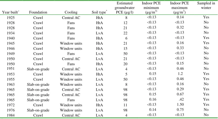
Table 2.1 shows the characteristics and minimum and maximum PCE concentrations measured in the 20 homes (all of which completed the study in its
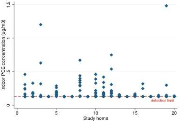
entirety). Figure 2.4 shows the detailed results for each house. PCE was detected in 12 of the 20 homes. The average PCE concentration across all samples above the detection limit was 0.28 µg/m3 (Table 2.2); however, concentrations fluctuated as much as one order of magnitude (Figure 2.5).
In general, the measured concentrations were low, although about half exceeded the EPA Region 6 risk-based screening level for resident air of 0.33 µ g/m3 that was in place at the time of sampling. In April 2012, the EPA revised its PCE screening level to 9.4 µg/m3, higher than all of the concentrations observed in this study. Nonetheless, the previous EPA analyses showing elevated subslab PCE concentrations and extremely low ambient concentrations (Figure 2.1) suggests that vapor intrusion may be an important source of the PCE observed in these homes, particularly because we removed indoor sources prior to sampling. (As an additional check on potential indoor sources, we also examined the correlations between measured PCE concentrations and self-reported days when cleaning products were used, but none of these correlations was significant.) Neither field blanks nor laboratory method blank samples had any measurable
Table 2.1. Characteristics of the 20 homes included in this study.
Year built+ Foundation Cooling Soil type*
Estimated groundwater
PCE (µg/l)
Indoor PCE minimum
(µg/m3)
Indoor PCE maximum
(µg/m3)
Sampled in winter
1925 Crawl Central AC HtA 8 <0.13 0.14 Yes
1928 Crawl Fans HtA 12 <0.13 <0.13 No
1928 Crawl Fans HtA 21 <0.13 0.32 No
1934 Crawl Fans LvA 22 <0.13 <0.13 No
1940 Crawl Fans HtA 6 <0.13 <0.13 Yes
1945 Crawl Window units HtA 21 <0.13 0.16 Yes
1946 Crawl Window units HtA 15 <0.13 0.33 No
1949 Crawl Fans LvA 50 <0.13 <0.13 No
1950 Crawl Central AC LvA 21 <0.13 <0.13 No
1950 Crawl Fans HtA 20 <0.13 0.15 No
1951 Slab-on-grade Central AC LvA 4 <0.13 0.46 No
1953 Crawl Window units HtA 5 0.15 1.2 Yes
1955 Crawl Window units LvA 50 <0.13 0.46 Yes
1963 Slab-on-grade Window units LvA 8 <0.13 0.16 No
1965 Slab-on-grade Central AC LvA 98 <0.13 0.29 Yes
1965 Slab-on-grade Central AC LvA 98 0.15 0.67 Yes
1965 Slab-on-grade Fans LvA 98 0.16 .42 Yes
1972 Crawl Window units HtA 11 <0.13 1.50 Yes
1976 Slab-on-grade Window units LvA 98 0.14 0.75 No
1984 Crawl Central AC LvA 4 <0.13 <0.13 No
Figure 2.4. Indoor air concentration of PCE by study home.
Table 2.2. Summary statistics for the key continuous variables included in the regression
model.
Time-variant variables Above detection samples (ns=90)
Below detection samples (ns=106)
PCE concentration
Indoor air (µg/m3) 0.28 (0.22)+
≤0.13 -- Weather characteristics
Barometric pressure drop (mm Hg) Average wind speed (m/s)
Relative humidity (%)
6.05 (2.53) 4.03 (0.89) 62.64 (14.53) 5.91 (2.63) 4.32 (0.86) 58.2 (11.98) Time Invariant Variables Houses with any sample above
the detection limit (nh=12)
Houses with no samples above the detection limit (nh=8)
PCE in the groundwater
Groundwater concentration (µg/L) 43.6 (40.2)
32.8 (29.1) Household characteristics
House area (m2) House age (years)
Figure 2.5. Temporal variation in indoor PCE concentrations in homes with at least one
sample above the detection limit.
2.3.1. Within-Home Temporal Variability
effects of rainfall, such as groundwater rise. During rain events, humidity levels exceed 90%, while the average during the study period was 62%. In summary, for this
community based on the regression analysis, it is expected that PCE concentrations in homes that are prone to vapor intrusion PCE concentrations will be higher during summer, during low-wind events, or when large barometric pressure drops occur.
Table 2.3. Average marginal effects for the within-home variability of natural log PCE
indoor air concentration (ln-µg/m3) due to vapor intrusion.
Covariate Coefficient+
Weather characteristics
Barometric pressure drop (mm Hg) Average wind speed (m/s)
Relative humidity (%) Relative humidity squared (%) Winter season 0.11* (0.051) -0.26** (0.093) 0.29** (0.017) -0.0017 (0.00051) -2.50** (0.71)
Constant -12.42**
(2.48)
Note: There were 120 observations from 13 homes. Standard errors (in parentheses) were computed using clustered robust standard errors.
+McFadden’s pseudo R2: 0.2887. F-statistic: 3.98 (p<0.0001) * Statistically significant at the 5% level.
** Statistically significant at the 1% level.
2.3.2. Spatial (Between-Home) Variability
as a quadratic term, p=0.04). On the other hand, concentrations decrease in the absence of an air conditioning unit (presumably because windows are opened, p=0.015) and with wind speed (p=0.004). Although not statistically significant, larger homes tended to have higher indoor PCE concentrations, while lower PCE concentrations were measured in older (and presumably leakier) homes. Together, all of these included covariates are highly significant (p<0.001).
Table 2.4. Population-averaged effects of model covariates on between-home (spatial)
variability of natural log PCE indoor air concentration (ln-µg/m3) due to vapor intrusion.
Variable Coefficient+
PCE concentration
Log of groundwater concentration (log-µg/L)
0.16* (0.07) Household characteristics
Slab-on-grade foundation No air conditioning units House area (m2)
Age of home (years)
0.83* (0.37) -0.51* (0.20) 0.0017 (0.0019) -0.0060 (0.0057) Environmental characteristics
Houston Black clay soil -0.46*
(0.23) Weather characteristics
Barometric pressure drop (mm Hg) Average wind speed (m/s)
Humidity (%)
Relative humidity squared (%) Winter season 0.15* (0.07) -0.36** (0.12) 0.051* (0.02) -0.002** (0.0006) -2.84** (1.01)
Constant -4.45**
(1.13)
Note: There were 182 observations from 20 homes. Clustered robust standard errors in parenthesis. +McFadden’s pseudo R2: 0.3389. F-statistic: 7.96 (p<0.0001)
2.4. Discussion
The indoor air concentrations observed in this study were similar to the results previously found in the EPA investigation (see Figure 2.1). The highest concentration measured by the EPA summa canister (1.83 µ g/m3) was on par with the highest
observations in this study (1.50 µg/m3). We do, however, observe a short-term temporal variability in indoor air concentrations that cannot be captured with a single-point-in-time sampling event. The relationship between meteorological conditions and indoor PCE observed here could help indicate the potential range of concentrations when only a single measurement is possible.
Several previous studies have found relationships between meteorological variables and vapor intrusion similar to those observed here. Radon studies have shown that atmospheric pressure drops contribute to the total radon entry rate into a building and can increase indoor concentrations by a factor of two over a daily time scale (Holford, Schery, Wilson, & Phillips, 1993; Robinson, Sextro, & Riley, 1997). Although
advective mass transfer of hydrocarbons into the indoor air (Patterson & Davis, 2009). Our analysis also suggests that an ambient pressure drop may increase the mass of PCE flowing into the home.
The results of this study are limited by the small sample size and few homes studied compared with the size of the potentially affected population. Measurements were not taken during a rainstorm or during freezing conditions. The relationships identified here may not be generalizable to other sites, especially those with a different climate, hydrogeology, and housing stock. The homes included in the study were a convenience sample, not a random sample. Therefore, selection bias among the households that chose to participate in the study may have influenced the results of the analysis. The passive sampling devices showed relatively good precision, although in some cases the difference in the duplicates was high and the use of the average of the measurements may have biased the results. We did not collect summa canister samples (to compare the accuracy of the passive sampling devices), nor were ambient air samples collected. The sampling of the EPA and previous sampling by the local health department gave no indication of elevated ambient levels of PCE, but possible intrusion from outdoor sources may have affected our measurements.
Also worth noting are the potential advantages of the community-based research design used in this study. The study required daily access to each home and the
2.5. Conclusions
CHAPTER 3
Screening Houses for Vapor Intrusion Risks: A Multiple Regression Analysis Approach2
3.1. Introduction
When groundwater or soil contamination occurs near buildings, volatile
contaminants can migrate upwards and result in vapor-phase contaminant intrusion into the indoor air, a phenomenon called vapor intrusion. Chlorinated volatile organic compounds (CVOCs), which are among the most frequently detected groundwater
contaminants at hazardous waste sites in the United States, persist in the environment, are difficult to remediate, and hence may pose long-term exposure risks (Agency for Toxic Substances and Disease Registration, 2007; Fischer et al., 1996; McCarty, 2010; Simpkin & Norris, 2010; Travis & Doty, 1990).
Policy debates concerning how to evaluate and minimize vapor intrusion risks are ongoing. Key questions include (Schuver, 2007; U.S. Environmental Protection Agency, 2009):
1) What constitutes sufficient evidence of a complete vapor intrusion pathway? 2) How can those responsible for contaminated sites identify which homes are at
the highest risk for vapor intrusion?
2
Johnston, J.E., & MacDonald Gibson, J. 2013, in press. Screening houses for vapor
3) In which homes should vapor barriers, exhaust systems, or other measures be put in place in order to prevent exposure to vapors from subsurface
contaminants?
At many contaminated sites, hundreds or even thousands of buildings may be affected by vapor intrusion. Due to political, technical, and financial constraints, monitoring indoor air directly in every potentially affected home is typically infeasible. Hence, decision-makers employ screening tools to categorize buildings according to the level of potential vapor intrusion risk. The current draft U.S. Environmental Protection Agency (EPA) guidance document on vapor intrusion, released in 2002, proposes a sequential order of assessment steps to “screen in” sites for further, and increasingly more site-specific, investigation (U.S. EPA, 2002). The suggested protocol begins with an examination of the source of vapors (contaminated groundwater or unsaturated soils), proceeds to monitoring soil gas in the unsaturated zone above the source, and, if there is evidence of vapor intrusion, continues upward to collect samples at the exposure point (e.g., indoor air or sub-foundation vapor). Buildings may be designated as not requiring further investigation at any of these steps.
contaminant vapor migrates upward from the groundwater table, through the overlying soil, and into buildings; it is defined as (Johnson & Ettinger, 1991):
α=Cindoor
Csource (1)
where
C
indoor is the contaminant concentration in indoor air (mass/volume) andC
sourceis the contaminant concentration in the soil gas just above the water table (mass/volume). Currently, the EPA recommends employing a generic attenuation factor of 1/1,000 to every building where the groundwater table is at least 5 feet from the ground surface, implying a contaminant concentration decrease of at least three orders of magnitude as the contaminant migrates upward into the building.Previous reviews of empirical data at vapor intrusion sites have identified
measured attenuation factors that range over several orders of magnitude. A comparison of attenuation factors found values as high as 0.1, with site averages ranging from 10-6 to 10-2 for chlorinated solvents (Johnston & MacDonald Gibson, 2011). Such results suggest that a factor of 1/1,000 could underpredict vapor intrusion risks (i.e., not be sufficiently conservative) in some cases. Others have suggested that the EPA generic attenuation factor is overly conservative—that, in practice, observed attenuation factors usually are significantly lower than 1/1,000 (Folkes, Kurtz, & Wannamaker, 2007; Johnson, Ettinger, Kurtz, Bryan, & Kester, 2009).
substantial spatiotemporal variability observed empirically(Bozkurt, Pennell, & Suuberg, 2009; Hers, Zapf-Gilje, Evans, & Li, 2002; Hers & Zapf-Gilje, 2003; Johnson, 2005; McDonald & Wertz, 2007; Pennell, Bozkurt, & Suuberg, 2009; Tillman & Weaver, 2006).
In order to provide a data source for further studying factors that influence vapor intrusion, the EPA compiled the National Vapor Intrusion Database. This database represents the largest collection of vapor intrusion data in the United States (Dawson, 2008b; U.S. EPA, 2012), containing as of 2012 almost 2,400 indoor air observations collected during 1990-2007 in 913 buildings at 41 sites in 15 states. EPA personnel reviewed and quality-assured the data prior to inclusion in the database (U.S. EPA, 2012). The data represent a cross-sectional collection of vapor intrusion observations; most sites do not include multiple measurements in multiple buildings over time. A detailed description of the database, data sources, and included parameters is available from U.S. EPA’s (2012) vapor intrusion database report.
This paper provides the results of the first systematic multivariate analysis of the EPA’s vapor intrusion database. We employ a multivariate regression approach to evaluate the effects of contaminant properties, geologic conditions, groundwater depth, soil type, building foundation type, and season on the observed vapor attenuation factors. Our analysis focuses on chlorinated solvents, which are among the most common
3.2. Methods
3.2.1. Dependent Variable
The dependent variable in this analysis is the attenuation factor (Equation 1). Hence, only observations for which paired data on groundwater and indoor air contamination were available were eligible for inclusion (~35% of the data). Using average groundwater temperature and adjusted chemical-specific Henry’s constants, the measured groundwater concentrations were converted into groundwater-source vapor concentrations (µg/m3), and then calculated the groundwater vapor intrusion attenuation factor as follows:
αi = Ci,indoor Ci,gw×KH ,i×1000L
m3
(2)
where
α
i is the vapor attenuation factor for chemical i, Ci,indoor is the concentration of the chemical i indoors due to vapor intrusion (µg/m3), Cgw is the concentration of thecontaminant in the groundwater (µg/L), and KH,i is the chemical-specific Henry’s constant for the average temperature of the groundwater (unitless). As Johnson et al. (2009) recommend, in order to avoid biasing the results we excluded samples with groundwater or indoor air concentrations below the detection limit.
CVOCs are often detected in indoor air even in areas not affected by
of indoor sources) (Dawson & McAlary, 2009; Johnson et al., 2009; U.S. EPA, 2012). Our analysis excluded these observations.
3.2.2. Explanatory Covariates
Covariates in this analysis included geological, environmental, household, and chemical characteristics. We grouped contaminated sites into six geological groundwater regions, reflecting similarities in the composition, arrangement, and structure of
subsurface formations as well as in broad water storage and transmission characteristics (Heath, 1984). Other environmental covariates were the depth to groundwater (m) and soil type. Soil type was classified as fine-grained (predominantly clay or silts), coarse (sandy soils), or very coarse (sand plus pebbles or rocks) generally based on the coarsest soil described in the vadose zone at the site.
Four types of foundations typified buildings in the database and hence also were considered as covariates: basement, slab-on-grade, crawl space, or partial basement. Buildings were further divided into residential, mixed-use, or commercial/institutional. In the final model, 96% of the observations were categorized as residential, so we restricted the analysis to residential buildings.
Seven CVOCs were included in the final analysis: dichloroethane, 1,1-dichloroethylene (DCE), 1,1,1-trichloroethane, cis-1,2-1,1-dichloroethylene,
tetrachloroethylene (PCE), trichloroethylene (TCE), and vinyl chloride. Since the chemical properties are important parameters in fate and transport models, we
3.2.3. Statistical Analysis
Since the attenuation factors were right skewed, the regression analysis employed the logarithm of the observed attenuation factor as the dependent variable (see Appendix B, Figure B.1). The associations between the vapor intrusion attenuation factor and environmental parameters, household characteristics, and chemical properties were then explored using multivariate statistical techniques, as described in the following sections.
Multivariate Regression Model
Our first regression analysis fitted the following model to the pooled data:
log yi=αααα+Bxi+εεεεi (4)
where yi is the vapor intrusion attenuation factor for observation i,
x
i is the vector of model covariates, Β is the vector regression coefficient, andε
i is the residual vector. The data exhibit positive spatial autocorrelation (the tendency for measurements in close spatial proximity to share similar attributes). Classical regression techniques applied to such mixed-level data often exaggerate levels of statistical significance of coefficient estimates (Moulton, 1990; Wooldridge, 2003). Our first multivariate pooled regression approach controlled for such site-level clustering by adjusting the standard error,Multilevel Regression Model
Second, we implemented a multilevel linear regression model that views the data as arising from a hierarchical process in which individual buildings are nested within sites that share common characteristics and sites are, in turn, nested in regions with geologic similarities (Figure 3.1). Multilevel statistical techniques provide a technically robust analytical framework when the causal processes that affect the outcome are hypothesized to operate in such a nested fashion (Gelman & Hill, 2006; Subramanian, Jones, & Duncan, 2003). Exploratory analysis of the attenuation factor data suggests that a hierarchical framework may be appropriate (see Appendix B, Figure B.2). For
hierarchical data, a pooled regression estimator of the effect of an observation-level predictor may be biased when using a flat regression approach such as in our first model (Steenbergen & Jones, 2002). The multilevel approach allowed us to examine the
Figure 3.1. Schematic of nested multilevel model.
The multilevel approach models the intercept of each level as random, assuming that building i is nested within site j, which in turn is nested within geological region k:
log yijk =ππππ0 jk+ ππππpjk p=1
P
∑
xpjk+εεεεijk(5) where π0jk is the intercept, πpjk is the vector of regression coefficients and xpijk is the vector of explanatory variables at the observation level. Assuming there are Q level-2 predictors and allowing zqjk to be the qth predictor in site j influencing attenuation, then the model is further specified as:
π0 jk =β00k + β0qk
q=1
Q
∑
zqjk +δ0 jk(6)