ADVANCED BAYESIAN MODELS FOR HIGH-DIMENSIONAL BIOMEDICAL DATA
Eunjee Lee
A dissertation submitted to the faculty of the University of North Carolina at Chapel Hill in partial fulfillment of the requirements for the degree of Doctor of Philosophy in the
Department of Statistics and Operations Research.
Chapel Hill 2016
c 2016 Eunjee Lee
ABSTRACT
EUNJEE LEE: ADVANCED BAYESIAN MODELS FOR HIGH-DIMENSIONAL BIOMEDICAL DATA
(Under the direction of Joseph G. Ibrahim and Hongtu Zhu)
Alzheimer’s Disease (AD) is a neurodegenerative and firmly incurable disease, and the total number of AD patients is predicted to be 13.8 million by 2050 [68]. Our motivation comes from needs to unravel a missing link between AD and biomedical information for a better understanding of AD. With the advent of data acquisition techniques, we could obtain more biomedical data with a massive and complex structure. Classical statistical models, however, often fail to address the unique structures, which hinders rigorous analysis.
ACKNOWLEDGEMENTS
My Ph.D. journey could not be completed without my advisors Professor Hongtu Zhu and Professor Joseph Ibrahim. Professor Ibrahim introduced Bayesian statistics and survival analysis with his motivation, immense knowledge, and patience. He guides me from very small details to main idea on my dissertation. Professor Zhu was always there whenever I was in trouble. I was inspired by his expertise in (say everything but in particular) statistical methods for neuroimaging and genetic data. He cared and encouraged what I did, and it helped me to finish my dissertation.
I would like to thank my committee members, Professor Jan Hannig, Professor Yufeng Liu, and Professor Sonia Davis for their insightful comments and encouragement. Professor Hannig’s insights helped me to think further on Bayesian methods. Professor Liu’s comments were very helpful to understand high-dimensional and functional data. Professor Davis’s (written and verbal) comments improved my dissertation a lot. Her expertise in Alzheimer’s disease helped me to find a better direction in the data analysis.
Thank you Professor Ja-Yong Koo for encouraging me. You helped me to start and finish my Master’s and Doctoral degrees and I learnt how to do research from you.
Thank you my husband Kibok for encouraging me all the time. I could not overcome hard times without your support. Thanks for being a very good listener when I practiced presentations.
Thank you my parents for being my parents. My life is full of love because you have always cheered me up. I hope that this achievement will be a small gift to you.
I met good friends during the five years in Chapel Hill.
• Thanks to Sunyoung for everything. You were the first person that I could contact when I was in trouble (well, except for my husband).
• Thanks to Hana, for being my friend. I laughed a lot when I talked with you. Also, your advise for my interviews was excellent!
• Jung In, you were friendly to me. I was so happy when we went to the Duke garden this Spring. Hope that we could meet in another lovely place.
• Thanks to Sieun, for having all the nice times with me: I remember a small concert in Carrboro. I will miss you so much.
• Hyosun, I enjoyed talking with you. I will miss our happy times in Spanky’s. We came to UNC in 2011 and made it finally! I am so proud of you.
• Mihye, I could smoothly start my research in the lab because you helped me a lot. We have had nice times in many cities and we will do more.
• Eunhwa, you were such a good friend. Our weekly routine to study is unforgettable. Thanks for being on my side all the time.
• Thanks to Hanseul for cheering me up. You have supported me and now I will do it for you. I miss our memory in NC.
• Soyoung, thanks for always cheering me up when I had hard times.
• Hyo Young and Duyeol, thanks for having good times with me in Chapel Hill. For my defense, Duyeol helped me to set-up the snacks and it was just perfect.
• Thanks to Wan Suk for helping me a lot. I was so thankful when you brought a cable before my defense. I got very relieved because I had what I needed!
• Hojin, thanks for your help when we were in the lab.
PREFACE
TABLE OF CONTENTS
LIST OF TABLES... xi
LIST OF FIGURES...xiv
1 INTRODUCTION... 1
1.1 Bayesian Functional Cox Regression Model... 2
1.2 Bayesian Bi-level Variable Selection with Censored Outcomes ... 4
1.3 Bayesian Hierarchical Group Spectral Clustering ... 5
2 LITERATURE REVIEWS... 8
2.1 Survival Analysis... 8
2.2 Proportional Hazards Model ... 9
2.3 Accelerated Failure Time Model ... 10
2.4 Functional Linear Regression ... 11
2.4.1 Functional Data and Smoothing... 11
2.4.2 Model Setup ... 12
2.4.3 Estimation of Functional Coefficients ... 12
3 BAYESIAN FUNCTIONAL LINEAR COX REGRESSION MODELS ... 15
3.1 Introduction ... 15
3.2 Bayesian Functional Linear Cox Regression Models ... 18
3.2.1 Setup ... 18
3.2.2 Model Formulation ... 20
3.2.3 Priors ... 21
3.3 Alzheimer’s Disease Neuroimaging Initiative Data Analysis... 24
3.3.1 Alzheimer’s Disease Neuroimaging Initiative... 24
3.3.2 Data Description ... 25
3.3.3 Hippocampus Image Preprocessing ... 27
3.3.4 Data Analysis ... 28
3.3.5 Sensitivity Analysis ... 33
3.4 Simulation Studies ... 34
3.4.1 Setup ... 34
3.4.2 Simulation Results... 35
3.5 Discussion ... 38
3.6 Supplementary: Posterior Estimation Results for the Reduced Models... 42
4 BAYESIAN BI-LEVEL VARIABLE SELECTION IN SURVIVAL MODEL 52 4.1 Introduction ... 52
4.2 Accelerated Failure Time Model ... 54
4.3 Bayesian Bi-level Variable Selection in Accelerated Failure Time Model ... 55
4.3.1 The First Step: Groupwise Variable Selection... 57
4.3.2 The Second Step: Element-wise Variable Selection ... 60
4.4 Simulation Study ... 63
4.4.1 Setup ... 63
4.4.2 Simulation Results... 64
4.5 ADNI-1 Data Analysis ... 67
4.5.1 Sensitivity Analysis ... 72
4.6 Discussion ... 72
5 BAYESIAN HIERARCHICAL GROUP SPECTRAL CLUSTERING... 76
5.1 Introduction ... 76
5.2.1 Model Formulation ... 78
5.2.2 Bayesian Approach ... 80
5.3 Simulation study ... 84
5.3.1 Simulation 1 ... 84
5.3.2 Simulation 2 ... 87
5.4 Application to Alzheimer’s Disease... 88
5.4.1 Data Acquisition and Pre-processing... 89
5.4.2 Data Analysis Results ... 90
5.5 Discussion ... 98
LIST OF TABLES
3.1 ADNI data analysis results for the full BFLCRM model: the posterior quanti-ties of 19 regression coefficientsβks, that correspond toxi =(Gender,
Handed-ness, Widowed, Divorced, Never married, Length of Education, Retirement, Age, APOE-4 carrier, ADAS-cog Score, posterior limb of internal capsule, Right hippocampal formation, Left hippocampal formation, Left thalamus, Left amygdala, Right amygdala, and Right thalamus). Mean denotes ‘poste-rior mean’, SD denotes ‘poste‘poste-rior standard deviation’, and lower and upper, respectively, represent the ‘lower and upper limits’ of a 95% highest posterior density interval. . . 29 3.2 ADNI data analysis results under the four models: DICs and the empirical
means of iAUC values and their corresponding standard errors in the paren-thesis calculated from the Monte Carlo cross-validation (MCCV). . . 32 3.3 ADNI data analysis results for Model 1: the posterior quantities of 12
regres-sion coefficientsβks, that correspond to xi =(Gender, Handedness, Widowed,
Divorced, Never married, Length of Education, Retirement, Age, APOE-4 carrier, and ADAS-cog Score). Mean denotes ‘posterior mean’, SD denotes ‘posterior standard deviation’, and lower and upper, respectively, represent the ‘lower and upper limits’ of a 95% highest posterior density interval. . . 32 3.4 Simulation results corresponding to h01(·) under different censoring rates and
sample sizes: the deviance information criterion (DIC), the mean squared errors (MSE) of ˆβ and ˆγ and the estimated integrated area under the curve (iAUCs) and their standard errors in parentheses calculated from the 100 simulated data sets. The Gibbs sampler was run for 20,000 iterations with 5,000 burn-in iterations for each simulated data set. . . 36 3.5 Simulation results corresponding to h01(·): the mean iAUC and the
corre-sponding standard error in the parenthesis calculated from the 100 simulated data sets for each scenario. The Gibbs sampler was run for 20,000 iterations with 5,000 burn-in iterations for each simulated data set. . . 36 3.6 Simulation results corresponding to h02(·) under different censoring rates and
3.7 Simulation results corresponding to h02(·): the mean iAUC and the corre-sponding standard error in the parenthesis calculated from the 100 simulated data sets for each scenario. The Gibbs sampler was run for 20,000 iterations with 5,000 burn-in iterations for each simulated data set. . . 38 3.8 ADNI data analysis results for Model 1: the posterior quantities of 10
regres-sion coefficientsβks, that correspond to xi =(Gender, Handedness, Widowed,
Divorced, Never married, Length of Education, Retirement, Age, APOE-4 carrier, and ADAS-cog Score). Mean denotes ‘posterior mean’, SD denotes ‘posterior standard deviation’, and lower and upper, respectively, represent the ‘lower and upper limits’ of a 95% highest posterior density interval. . . 43 3.9 ADNI data analysis results for Model 2: the posterior quantities of 17
regres-sion coefficientsβks, that correspond to xi =(Gender, Handedness, Widowed,
Divorced, Never married, Length of Education, Retirement, Age, APOE-4 carrier, ADAS-cog Score, posterior limb of internal capsule, Right hippocam-pal formation, Left hippocamhippocam-pal formation, Left thalamus, Left amygdala, Right amygdala, and Right thalamus). Mean denotes ‘posterior mean’, SD denotes ‘posterior standard deviation’, and lower and upper, respectively, rep-resent the ‘lower and upper limits’ of a 95% highest posterior density interval. 45 3.10 ADNI data analysis results for Model 3: the posterior quantities of 10
regres-sion coefficientsβks, that correspond to xi =(Gender, Handedness, Widowed,
Divorced, Never married, Length of Education, Retirement, Age, APOE-4 carrier, and ADAS-cog Score). Mean denotes ‘posterior mean’, SD denotes ‘posterior standard deviation’, and lower and upper, respectively, represent the ‘lower and upper limits’ of a 95% highest posterior density interval. . . 46 3.11 Sensitivity analysis of (β,γ) for ADNI-1 data with different values of
hyper-parameters in the Normal priors on the regression coefficients. . . 48 3.12 Sensitivity analysis of (β,γ) for ADNI-1 data with different values of
hyper-parameters in the Gamma priors on the piecewise constant baseline hazard function. . . 49 3.13 Sensitivity analysis of λ for ADNI-1 data with different values of
hyperpa-rameters in the Normal priors on the regression coefficients. . . 50 3.14 Sensitivity analysis ofλfor ADNI-1 data with different values of
hyperparam-eters in the Gamma priors on the piecewise constant baseline hazard function. 51
4.1 When the group-level variable selection performs perfectly, TP=10, FP=0, TPR=TNR=PPV=NPV=1. . . 65 4.2 When the element-wise variable selection performs perfectly, TPR=TNR=
4.3 Group-level selection results. When the group-level variable selection performs perfectly, TP=10, FP=0, TPR=TNR=PPV=NPV=1. . . 66 4.4 Element-wise selection results.When the element-wise variable selection
per-forms perfectly, TPR=TNR=PPV=NPV=1. . . 66 4.5 Bilevel selection results on ADNI-1 data: It shows the list of selected SNP-sets
associated with time to conversion from MCI to AD. For each selected group, the corresponding bp ranges, the number of SNPs, and gene names are shown. 70 4.6 Sensitivity analysis ofλfor ADNI-1 data with different values of
hyperparam-eters in the IM/IMR priors within the group-level selection. . . 73 4.7 Sensitivity analysis of c0 for ADNI-1 data with different values of
hyperpa-rameters in the IM/IMR priors within the group-level selection. . . 74
5.1 In order to select the number of common factors, we used BIC. TP and FP denote the number of true positive and the number of false positive, respectively. 85 5.2 In order to select the number of common factors, we used BIC. TP and FP
denote the number of true positive and the number of false positive, respectively. 86 5.3 Estimation error for Γ0 and Γ1 in the two different cases. They are mean
LIST OF FIGURES
3.1 ADNI data: panel (a) is hippocampal subfields mapped onto a repre-sentative hippocampal surface [5], and panels (b) and (c), respectively, show the top and bottom views of the first subject’s hippocampal sur-face data where the corresponding radial distances are color-coded by
the colorbar in panel (d). . . 19 3.2 ADNI data analysis results for the full BFLCRM model: panels (a)
and (b), respectively, show the top and bottom views of the esti-mated coefficient function associated with the hippocampal surface
data color-coded by the colorbar in panel (c). . . 30 3.3 ADNI data analysis results: the estimated survival curves of
4 carriers and non-carriers under the full BFLCRM model. Other continuous or categorical covariates are fixed at the mean values or reference levels. The dotted lines show the 95% HPD intervals of the
estimated survival functions. . . 31 3.4 Simulation results corresponding toh01(·): panels (a) and (b)
respec-tively show the first 10 estimated baseline hazard functions with 0.3 and 0.5 censoring rates based on the size 500 samples. The solid line
is the true baseline hazard function,h01(·). . . 37 3.5 Simulation results corresponding toh02(·): panels (a) and (b)
respec-tively show the first 10 estimated baseline hazard functions with 0.3 and 0.5 censoring rates based on the size 500 samples. The solid line
is the true baseline hazard function,h02(·). . . 39 3.6 ADNI data analysis results: the estimated survival curves of
4 carriers and non-carriers under the full and reduced BFLCRM models. Other continuous or categorical covariates are fixed at the mean values or reference levels. The dotted lines are the 95% HPD
intervals of the estimated survival functions. . . 44 3.7 ADNI data analysis results for Model 1: panels (a) and (b),
respec-tively, show the top and bottom views of the estimated coefficient function associated with the hippocampal surface data color-coded
by the colorbar in panel (c). . . 45 3.8 ADNI data analysis results: the first 12 largest estimated
4.1 Posterior inclusion probabilities of 16,106 SNP-sets. Our proposed method identified 19 important SNP-sets after Bayesian FDR
correc-tion. The solid line shows the FDR criteria, 0.941 in this data. . . 68 4.2 Estimated coefficient values for 795 SNPs included in the 19
SNP-sets. We highlighted 106 selected SNPs in the elementwise-selection
step. . . 69 4.3 Trace and ACF plots of the regression coefficients of the first selected
SNP-set θ1,1, θ1,2, and θ1,3 are respectively plotted in panels (a), (b), and (c) for 5000 iterations of the MCMC algorithm. The trace plots show fast convergence of the algorithm, indicating its good mixing
properties. . . 69 4.4 A manhattan plot with -log 10(p-value) for the simple GWAS. The
solid line shows the 5×10⁻⁸ significance level. . . . 71
5.1 Figure (a) shows the first raw data matrix L1 in the first simula-tion data set, while figure (b) shows the approximated matrix by the
proposed method. . . 85 5.2 Figure (a) shows the first raw data matrix Li in the first
simula-tion data set, while figure (b) shows the approximated matrix by the
proposed method. . . 86 5.3 It shows process to estimate functional connectivity from resting-state
fMRI data. . . 89 5.4 It shows BIC values for the different number of underlying factors.
The optimal number can be selected as 15. . . 91 5.5 Figure (a) shows the estimated B matrix with standardized scale,
while figure (b) shows the standardized B matrix after thresholding
the absolute values at 2.1. . . 91 5.6 It shows how the raw correlation matrix of the first subject can be
decomposed by the BGSC. . . 92 5.7 It shows which connectivity is different between MCI and AD groups.
The red line represents the estimated coefficient value γ4−γ3 > 0, which implies that AD patients have a stronger positive connection than MCI subjects between the corresponding two ROIs. The blue line represents the estimated coefficient value γ4 − γ3 < 0 indicat-ing that AD patients have a weaker positive connection than MCI
5.8 It shows which connectivity is different between MCI and AD groups. The red line represents the estimated coefficient value γ4−γ3 < 0, which implies that AD patients have a stronger negative connection than MCI subjects between the corresponding two ROIs. The blue line represents the estimated coefficient value γ4 − γ3 > 0 indicat-ing that AD patients have a weaker negative connection than MCI
subjects between the corresponding two ROIs. . . 95 5.9 Trace and ACF plots of Λ1(1,1), Λ1(1,2), and Λ1(1,3) are respectively
plotted in panels (a), (b), and (c) for 5000 iterations of the MCMC algorithm. The trace plots show fast convergence of the algorithm,
indicating its good mixing properties. . . 96 5.10 Trace and ACF plots of Γ3(1,1) and Γ4(1,1) are respectively plotted
in panels (a) and (b) for 5000 iterations of the MCMC algorithm. The trace plots show fast convergence of the algorithm, indicating its
good mixing properties. . . 96 5.11 Trace and ACF plots of σ2, σ2
0, and σγ2 are respectively plotted in
panels (a), (b), and (c) for 5000 iterations of the MCMC algorithm. The trace plots show fast convergence of the algorithm about 200
iterations, indicating its good mixing properties. . . 98 5.12 It shows which connectivity is different between NC and MCI groups.
The red line represents the estimated coefficient value γ3 >0, which implies that MCI patients have a stronger positive connection than NC subjects between the corresponding two ROIs. The blue line represents the estimated coefficient valueγ3 <0 indicating that MCI patients have a weaker positive connection than NC subjects between
the corresponding two ROIs. . . 99 5.13 It shows which connectivity is different between NC and MCI groups.
The red line represents the estimated coefficient value γ3 <0, which implies that MCI patients have a stronger negative connection than NC subjects between the corresponding two ROIs. The blue line represents the estimated coefficient valueγ3 >0 indicating that MCI patients have a weaker negative connection than NC subjects between
the corresponding two ROIs. . . 100 5.14 It shows which connectivity is different between NC and AD groups.
The red line represents the estimated coefficient value γ4 >0, which implies that AD patients have a stronger positive connection than NC subjects between the corresponding two ROIs. The blue line represents the estimated coefficient value γ4 <0 indicating that AD patients have a weaker positive connection than NC subjects between
5.15 It shows which connectivity is different between NC and AD groups. The red line represents the estimated coefficient value γ4 <0, which implies that AD patients have a stronger negative connection than NC subjects between the corresponding two ROIs. The blue line represents the estimated coefficient value γ4 >0 indicating that AD patients have a weaker negative connection than NC subjects between
CHAPTER 1
INTRODUCTION
Alzheimer’s Disease (AD) is a neurodegenerative and firmly incurable disease, and the total number of AD patients is predicted to be 13.8 million by 2050 [68]. Our motivation comes from needs to unravel a missing link between AD and biomedical information for a better understanding of AD. With the advent of data acquisition techniques, we could obtain more biomedical data with a massive and complex structure. Classical statistical models, however, often fail to address the unique structures, which hinders rigorous analysis
A fundamental question this dissertation is asking is how to use the data in a better way. Bayesian methods for high-dimensional data have been successfully employed by using novel priors, MCMC algorithms, and hierarchical modeling. This dissertation proposes novel Bayesian approaches to address statistical challenges arising in biomedical data including brain imaging and genetic data.
progression to AD. While hippocampus and genetic variants are important risk factors, many classical survival models are not theoretically and computationally suitable because they take the forms of functional and high dimensional data. Motivated by the limitations of classical survival models, this dissertation proposes survival models with functional or high dimensional covariates by taking a Bayesian approach. In order to make use of functional data as covariates to predict the time to event, a Bayesian functional linear Cox regression model is proposed in Chapter 3. In Chapter 4, we propose Bayesian bi-level variable selection to enable variable selection in both group and element levels for high-dimensional predictors. In the following sections, we discuss brief motivation and description of the two modern survival models.
The second part discusses a Bayesian matrix decomposition method applicable to brain functional connectivity. Functional connectivity is the connectivity between different brain areas sharing information and functions [153]. It can be estimated by pairwise temporal cor-relation between two spatially remote BOLD signals in rsfMRI. It is an important biomarker in psychiatric disorders because its abnormality has been observed in subjects with brain disorders including AD, schizophrenia, and ADHD [58]. One specific question will be“is there any relationship between altered functional connectivity and neurological disorders?”. In Chapter 5, we propose a Bayesian hierarchical group spectral clustering model to analyze brain connectivity. It facilitates estimation of clinical covariates, which enables to examine if functional connectivity had group difference among normal, MCI, and AD subjects. 1.1 Bayesian Functional Cox Regression Model
global measure. It is the distance from medial core of the hippocampus to its surface, which takes the form of 2-dimensional curve quantifying the thickness of hippocampus relative to its centerline. By comparing the radial distance of different individuals, the relative atrophy against each other can be measured. Apostolova et al. [6] have shown that MCI patients who progress to AD have smaller hippocampi around CA1 region than MCI patients who does not develop AD. Also AD patients tend to have a higher annual atrophy rate on few regions of CA1 than MCI patients [51].
Since the hippocampal radial distance is a 2-dimensional curve, which can be considered as functional data, classical regression models should be adapted to incorporate functional covariates. In order to describe the nature of functional data as covariates in linear models, functional linear regression has been proposed and discussed in many literatures including Cardot et al. [19], Ramsay and Silverman [131], M¨uller and Stadtm¨uller [114]. Functional covariates can be estimated by employing functional principal component analysis (fPCA) on a continuous covariance function of the functional covariates [19, 114, 18]. In the generalized linear model framework, M¨uller and Stadtm¨uller [114] apply a Karhunen-Loeve expansion on the functional predictor, which enables dimension reduction to a finite number of components of the expansion. More reviews regarding functional regression models will be discussed in section 2.2.
1.2 Bayesian Bi-level Variable Selection with Censored Outcomes
Since AD is highly heritable, genome-wide association studies (GWASs) have been con-ducted for the purpose of identifying genetic variants contributing to AD. Typically, it is of interest to elucidate the association between the traits and single-nucleotide polymorphisms (SNPs), a DNA sequence variation occurring commonly within a population. A genome-wide association study (GWAS) focuses on identifying important SNPs to relate to clinical outcomes in this context. Since the SNP data is ultra high-dimensional (half a million or more), the simple (and popular) GWASs conduct a number of marginal tests: examination of the effect of each SNP one by one. It makes GWAS to be theoretically and computationally feasible in the classical regression setup, p <n, where p is the number of covariates and n is the number of observations. But the simple GWASs face two main challenges: dealing with multiple testing issue and accounting for the dependency structure among SNPs.
and slab priors. Bayesian variable selection approach [138] and Bayesian LASSO [92] are considered in the AFT model. But these methods do not take into account any grouping information among predictors.
In order to tackle the limitations that the existing variable selection methods have in the context of GWAS, we propose a Bayesian bi-level variable selection (BBVS) method in the accelerated failure time model in Chapter 4. Our main goal is (1) identification of SNPs associated with time to conversion from MCI to AD (2) by considering all the SNPs simultaneously and (3) incorporating the grouping information of the SNP data. Our method has two hierarchical levels of variable selection: the first one is group-wise and the second level is element-wise variable selection. In the first step, we identify important groups of variables and update the censored event time from its predictive posterior distribution by data augmentation [150, 138]. The dimension of the whole SNP data can be significantly reduced by eliminating irrelevant groups to time to event. Since this step also provides a posterior sample of censored time to event, the posterior mean will be used as imputed censored event time in the second level of variable selection. It converts the AFT model in the second level into a usual log-normal regression model. In the second level, we only include variables in the selected groups as covariates in the AFT model with the imputed event time as an outcome. To conduct element-wise variable selection, shrinkage priors are employed on regression parameters. In particular, we extend Dirichlet-Laplace shrinkage priors proposed by [9] to incorporate the grouping information.
1.3 Bayesian Hierarchical Group Spectral Clustering
Functional connectivity is the connectivity between different brain areas sharing informa-tion and funcinforma-tions [153]. Unraveling a missing link between neurological disorder and brain network is an ongoing quest in various fields including statistics, epidemiology, and neuro-science. One specific question will be “is there any relationship between altered functional connectivity and neurological disorders?”. There are two main standard methods to tackle the question: univariate approaches to see if each correlation (node) has group difference using Fisher’s z-transformation, and graph theoretical approaches based on some summary statistic for a network structure (i.e., girth, diameter, modularity, small-worldness). The first method easily faces high-dimensional multiple testing problem. If there is a small group dif-ference in each correlation, the univariate approach is likely to miss the signal, which results in low power. Also, it discards a spatial structure among close or related brain regions (vox-els). The second methods often fail to detect local differences among subject groups, because the connectivity structures are too simplified by the summary statistics. Thus, alternative connectivity analysis methods are critically needed.
taken into account to have meaningful signals.
We propose a Bayesian hierarchical group spectral clustering model to take a global ap-proach to analyze brain connectivity. We decompose a correlation matrix (possibly it can be any symmetric matrix) with underlying common factors across subjects and the subject-specific coefficient matrix (Λi). TheΛi matrix preserves an individual network structure in
the low-dimensional space spanned by the common factors. One more intriguing part is a hi-erarchical structure within a prior ofΛi in order to estimate effects of clinical/demographic
CHAPTER 2
LITERATURE REVIEWS
2.1 Survival Analysis
In survival analysis, the outcome of interest is the survival times of subjects. The sur-vival times are denoted by T, a continuous nonnegative random variable, with cumulative distribution functionF(t) on the interval [0,∞). The probability that an individual survives till specified time point t is given by the survival function,
S(t) = 1−F(t) =P(T > t).
The survival functionS(t) is a monotone decreasing function withS(0) = 1 and limt→∞S(t) =
0. The hazard function h(t) is defined as the ratio of the probability density function f(t) to the survival function S(t), which is instantaneous rate of occurrence of the event. It can be written as
h(t) = lim
t→∞
P(t≤T < t+dt|T ≥t)
dt =
f(t)
S(t) (2.1.1)
Note thatf(t) = −d
dtS(t). Thus, (2.1.1) implies that h(t) = −d
dt logS(t). (2.1.2)
Integrating both sides of (2.1.2) and exponentiating give the following:
S(t) = exp
−
Z t
0
h(u)du
= exp(−H(t)),
where H(t) is is the cumulative hazard. From (2.1.2), it is derived that
f(t) =h(t) exp
−
Z t
0
h(u)du
2.2 Proportional Hazards Model
Survival models consist of two ingredients: the baseline hazard function, denoted h0(t) and the effect covariates. The baseline hazard function h0(t) quantifies how the risk of event per time unit varies over time when levels of covariates are fixed at baseline. The proportional hazards condition (Cox 1972) is that effect of a unit increase in a covariate is multiplicatively related to the hazard rate. Under the proportional hazards assumption, the effect of covariates can be estimated without taking into account the hazard function. The Proportional hazards model takes this approach on survival data. The hazard function of a subject at time t can be specified as
h(t|x) =h0(t) exp{x0β}, (2.2.1)
wherex= (x1,· · · , xp) is apcovariates vector andβ = (β1,· · · , βp) is a vector ofpregression
coefficients, and h0(t) is called the baseline hazard function. The model (2.2.1) implies that the ratio of hazards between two subjects is time-invariant and actually depends on the difference between their linear predictors,η=x0β. In biomedical research regarding survival data, some individuals are still alive or normal at the end of the study so death or occurrence of a disease has not happened. Therefore we have right censored data, that is, some of the survival times exceed a certain value. The certain time point is called a censoring time. The survival times tis are assumed to be independent and identically distributed with density f(t) and survival function S(t). Then survival time ti for the i-th subject will be observed only when ti ≤ ci, where ci is a fixed censoring time. The data D with a size n random
sample consists of (yi, νi, xi)ni=1, where yi = min(ti, ci), xi is the p×1 vector of covariates
function for (β, h0(·)) is given by
L(β, h0(t)|D) ∝
n
Y
i=1
[h0(yi) exp(x0iβ)] νi
S0(yi)exp(x
0 iβ) = n Y i=1
[h0(yi) exp(x0iβ)] νiexp
( n
X
i=1
exp(x0iβ)H0(yi)
)
,
where S0(t) is the baseline survivor function such that S0(t) = exp
−Rt
0 h0(u)du
= exp(H0(t)).
One of the most popular semiparametric survival models is a piecewise constant hazard model. On the time axis, we set a finite partition as 0 < s1 < · · · < sJ with sJ > yi for all i = 1,· · · , n, where s0 = 0. In the j-th interval, we assume a constant baseline hazard
h0(y) = λi for sj1 < y ≤sj. Then the likelihood function can be written as
L(β,λ|D) =
n Y i=1 J Y j=1
[λjexp(x0iβ)] uijνi
× n Y i=1 J Y j=1 exp "
−uij
(
λj(yi−sj−1)
j−1
X
g=1
λg(sg −sg−1)
)
exp(xi0β)
#
,
where uij = 1 if thei-th subject is right censored in the j-th interval and 0 otherwise.
2.3 Accelerated Failure Time Model
An accelerated failure time model (AFT model) is an alternative to the proportional hazards model. Since the proportional hazards model assumes a multiplicative effect on the hazard function, it is hard to interpret the estimates of regression parameters. The AFT model assumes a multiplicative effect on the time to event. For the i-th subject, its probability model is given by
Yi = exp(−x0iβ)νi, i= 1,· · · , n,
which becomes the linear model in log scale
where Y1, Y2,· · · , Yn are failure times,xi = (xi1, xi2,· · · , xip)0 is a vector of known
explana-tory variables for the i-th individual, β is a vector of p unknown regression coefficients, and i = logνi is the error term. Usually the error term is assumed to follow a parametric
distribution, such as the Normal distribution.
2.4 Functional Linear Regression
2.4.1 Functional Data and Smoothing
With the development of new technologies, data objects of interest are measured in a continuous time fashion. Functional data includes daily temperature data [131], Spectro-metric curves data, log-periodograms data [47], and many other objects in various fields. Since those data objects are curves, functional methods should be taken to analyze their global behavior. In practice, functional data is measured at (fine) discrete grid points. For a random function X(s), s ∈ S, we measure a discretized observation {W(sl)}Ll=1 at grid points {sl}Ll=1 ∈ S with measurement errors (sl). Assume that we have a random sample
{Xi(·)}ni=1, where the random functionsXi(·)s are independently and identically distributed
with the same distribution asXi(·). For the i-th observation,
Wi(sl) = Xi(sl) +i(sl) = µ(sl) + ¯Xi(sl) +i(sl),
whereXi(s) characterizes individual functional variations fromµ(s). Thei(s)s are
measure-ment errors with mean zero and variance σ2
(s) at each s and independent of each other for s 6=s0. Moreover, µ(s) can be consistently estimated by ¯µ(s) = Pn
i=1Wi(s)/n. To proceed
with functional data analysis, one needs to obtain a continuous smooth functional data by smoothing the discretized observations. We apply a cubic smoothing spline, which finds a minimizer f(x) of the following penalized residual sum of squares
n
X
i=1
L
X
l=1
(wil−fi(sl))0(wil−fi(sl)) +λ
Z
The second penalty term is the integrated squared second derivative and penalizes curvature in the function. Then a unique minimizer is a natural cubic spline with knots at the unique values of sl. In practice, we use the smoothed observations in the functional data analysis.
2.4.2 Model Setup
It is of interest to explain variation in a (scalar) response variable by relating with a functional covariate. We consider a linear regression setting, where the response variable
Y is a real-valued continuous random variable and the covariate X(s), s ∈ S, is a square integrable random function observed on S such that E(X(s)) = µ(s). The “functional” linear regression model can be expressed as
Y =β0+
Z
S
β(s)X(s)dt+,
where is are iid with E(|X(s), t ∈ S) = 0, Var(|X(s), t ∈ S) = σ2. A constant intercept
β0 is given byE(Y)−
R
Sβ(s)µ(s)ds. Without loss of generality, we assume that the variables
X(·) and Y are centered so that we have a simplified regression model
Y =
Z
S
β(s)X(s)dt+.
The coefficient function β(·) quantifies how much X(s) has an effect on Y across S, which is a major parameter in the functional linear model.
2.4.3 Estimation of Functional Coefficients
squared norm of a derivative given the order of the functional coefficient in the estimation step. The other widely used method is employing functional principal component analysis (fPCA) on a continuous covariance function of X(s) [19, 114, 18]. In the generalized linear model framework, M¨uller and Stadtm¨uller [114] apply a Karhunen-Loeve expansion on the functional predictor, which enables dimension reduction to a finite number of components of the expansion.
We review the fPCA approach in the functional linear regression setting. It is assumed that Xi(s) and i(s) are independent of each other and the covariance function of {Xi(s) : s∈ S}, denoted byK(s, s0) =E{X(s)X(s0)}, is continuous onS × S. According to Mercer’s theorem, K(s, s0) also admits a spectral decomposition
K(s, s0) =
∞
X
j=1
ψjφj(s)φj(s0),
where (ψj, φj(s))’s are the eigenvalue-eigenfunction pairs of K(s, s0) such that {ψj : j ≥
1} are the eigenvalues in decreasing order with P∞
j=1ψ 2
j < ∞. Thus, Xi(s) admits the
Karhunen-Loeve expansion as
Xi(s) =
∞
X
j=1
ξijφj(s),
where the ξij are referred to functional principal component (fPC) scores and the ξij =
R
SX(s)φj(s)dsare uncorrelated random variables with mean zero and variance ψj =E(ξij2).
To estimate ξij based on the observed covariate functions Wi(s), we first employ the cubic smoothing spline [65] to estimate the underlying signalXi(s). We then use the sample mean
and covariance functions of the estimatedXi(s) to estimateµ(s) andK(s, s0). Subsequently,
we estimate ψj(s) and ξij for all i, j ≤ n. Since the eigenfunctions ψj(·) form a complete
orthonormal system on the space of square-integrable functions onS, the covariate function
γ(s) can be expanded as
β(s) =
∞
X
j=1
φj(s)βj with
∞
X
j=1
Therefore, we have
Z
S
Xi(s)β(s)ds=
∞
X
i=1
ξijβj (2.4.2)
and with truncated linear predictors
Yi =
∞
X
i=1
ξijβj+i ≈ qn X
i=1
ξijβj +i, (2.4.3)
where qn is a sufficiently large integer that may depend on n. One can control smoothness of the functional coefficient by truncating the infinite summation in the equation (2.4.2) at the first qn summation. Since the approximation error of the truncated model is bounded
by the variance of the truncated part and is controlled by a sequence of eigenvalues, ψj,
the truncation step would allow nice approximation for the infinite summation. Practically, it is common to choose qn such that the percentage of variance explained by the first qn
CHAPTER 3
BAYESIAN FUNCTIONAL LINEAR COX REGRESSION MODELS
3.1 Introduction
Alzheimer’s Disease (AD) is a firmly incurable and progressive disease [36]. In the pathol-ogy of AD, mild cognitive impairment (MCI) is a clinical syndrome characterized by insidious onset and gradual progression, and commonly arising as a result of underlying neurodegener-ative pathology [53]. Since MCI is considered as a risk state for AD, a major research focus in recent years has been to delineate a set of biomarkers that provide evidence of such a neurodegenerative pathology in living individuals, with the goal of specifying the likelihood that the pathophysiological process is due to Alzheimer’s disease (MCI due to AD; MCI-AD) and will lead to dementia within a few years [1]. Accordingly, increasing attention has been devoted to investigate the utility of various imaging, genetic, clinical, behavioral, and fluid data to predict the conversion from MCI to AD.
Recently, most researchers have turned to the analysis of longitudinal data to assess the dynamic changes of various biomarkers associated with the MCI-to-AD transition across time. To begin, a prominent neural correlate of MCI-AD is volume loss within the MTL, especially within the hippocampus and entorhinal cortex [42], with increasing atrophy in these structures from normal aging to MCI to AD [123]. Longitudinal studies of individuals with MCI-AD have also highlighted the importance of assessing MTL changes in tracking the progression of MCI to AD. For example, several studies have documented diminished baseline hippocampal and entorhinal volumes that are associated with an increased likelihood of progressing to clinical dementia [85, 59]. Additionally, several modalities of disease indicators have been studied to assess progression to AD, including neuroimaging biomarkers [154, 166, 133], biomedical markers [139], and neuropsychological assessments [124]. Finally, a number of structural MRI studies, covering region of interest (ROI), volume of interest, voxel-based morphometry, and shape analysis have reported that the degree of atrophy in several brain regions, such as the hippocampus and entorhinal cortex, is not only sensitive to disease progression, but also predicts MCI conversion [28, 108, 40].
atrophy and ADAS-Cog offers good predictive power of conversion from MCI to AD, whereas APOE genotype did not significantly improve prediction. To the best of our knowledge, no prior study has examined the role of functional covariates including hippocampus surface morphology in predicting time to conversion from MCI to AD with/without adjusting for low-dimensional behavioral and clinical measures.
In Section 2, we will introduce BFLCRM and its associated Bayesian estimation proce-dure. In Section 3, we will introduce the NIH Alzheimer’s Disease Neuroimaging Initiative (ADNI) dataset and illustrate the use of BFLCRM in the prediction of time to conversion from MCI to AD by using both functional and scalar covariates. In Section 4, we conduct simulation studies to examine the finite sample performance of BFLCRM. In Section 5, we interpret the findings obtained from the analysis of ADNI dataset.
3.2 Bayesian Functional Linear Cox Regression Models
3.2.1 Setup
Consider imaging, genetic, and clinical data from n = 346 independent MCI patients in ADNI-1. For the i-th MCI patient, we observe a possibly right censored time to conversion to AD, denoted by yi. Specifically, yi = Ti ∧Ci is the minimum of the censoring time Ci and the transition time Ti and νi = 1(yi = Ti), where 1(·) is an indicator function.
Moreover, we observe a p×1 vector of scalar covariates, denoted by xi = (xi1,· · · , xip)T,
and a functional covariate, denoted by Zi(·), on a compact set S. In this paper, we focus
on the noninformative censoring setting such that Ti and Ci are conditionally independent given all covariates of interest. The scalar covariates of interest include age at baseline, length of education, gender, handedness, marital status, retirement, and the well-known Apolipoprotein E (APOE) SNPs. The APOE has three major forms, 2, 3, and 4, where
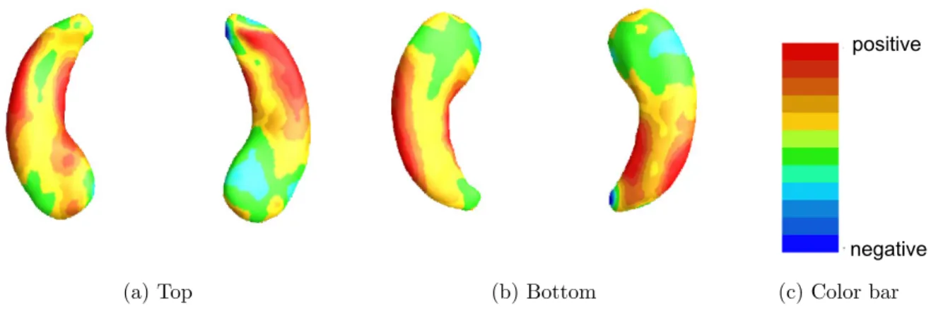
3 is the most common form. The functional covariate of interest is the hippocampus surface morphology. Figure 3.1 on page 19 shows the example hippocampus surface morphology data in ADNI-1 data.
CA1
CA2
CA3
Sub Sub
CA1
CA2
CA3
Sub Sub
Sub
CA1 CA1
Sub
(a) Hippocampal subfields
(b) Top (c) Bottom (d) Color bar
Figure 3.1: ADNI data: panel (a) is hippocampal subfields mapped onto a representative hippocampal surface [5], and panels (b) and (c), respectively, show the top and bottom views of the first subject’s hippocampal surface data where the corresponding radial distances are color-coded by the colorbar in panel (d).
sole presence of xi, it is common to consider Cox’s proportional hazards model [29], which
assumes that the conditional hazard function of yi given xi is given by
h(y|xi) = h0(y) exp(xTi β) = h0(y) exp
p
X
k=1
xikβk
!
, (3.2.1)
3.2.2 Model Formulation
We propose a Bayesian functional linear Cox regression model with three main ingredients for handling both functional and scalar covariates as a natural extension of (3.2.1). Based on this formulation, we take a Bayesian approach to estimate the parameters of interest.
In the first component of BFLCRM, it is assumed that the hazard function of yi given (xi, Zi(·)) is given by
h(y|xi, Zi(·)) =h0(y) exp
p
X
k=1
xikβk+
Z
S
γ(s)(Zi(s)−µ(s))ds
!
, (3.2.2)
whereµ(s) is the mean function ofZi(s) andγ(·) is an unknown coefficient function, a square integrable function on S.
The second component of BFLCRM is the functional principal component analysis (fPCA) model of the Zi(·)’s. It is assumed that the Zi(s)’s are square integrable random functions
and Wi(s) is measured at a set of grid points in S with measurement errors such that
Wi(s) = Zi(s) +i(s) = µ(s) + ¯Zi(s) +i(s), (3.2.3)
where ¯Zi(s) characterizes individual functional variations from µ(s). The i(s)’s are
mea-surement errors with mean zero and varianceσ2(s) at each s and independent of each other for s6=s0. Moreover, µ(s) can be consistently estimated by ˆµ(s) = Pn
i=1Wi(s)/n.
It is assumed that Zi(s) and i(s) are independent of each other and the covariance
function of {Z¯i(s) : s ∈ S}, denoted by K(s, s0) = E{Z¯(s) ¯Z(s0)}, is continuous on S × S.
According to Mercer’s theorem, K(s, s0) also admits a spectral decomposition K(s, s0) =
P∞
j=1ψjφj(s)φj(s0),where (ψj, φj(s))’s are the eigenvalue-eigenfunction pairs ofK(s, s0) such
that {ψj : j ≥ 1} are the eigenvalues in decreasing order with
P∞
j=1ψ 2
j < ∞. Thus, ¯Zi(s)
admits the Karhunen-Loeve expansion as ¯Zi(s) =P∞
j=1ξijφj(s), where theξij are referred to functional principal component (fPC) scores and the ξij =
R
random variables with mean zero and variance ψj = E(ξij2). To estimate ξij based on
the observed covariate functions Wi(s) , we first employ the cubic smoothing spline [65] to
estimate the underlying signalZi(s). We then use the sample mean and covariance functions
of the estimated Zi(s) to estimate µ(s) and K(s, s0). Subsequently, we estimate φj(s) and ξij for all i, j ≤n.
The third component of the BFLCRM is an approximation of RSγ(s) ¯Z(s)ds. Since the eigenfunctions ψj(·) form a complete orthonormal system on the space of square-integrable functions on S, the covariate function γ(s) can be expanded as
γ(s) =
∞
X
j=1
φj(s)γj with
∞
X
j=1
γj2 <∞. (3.2.4)
Therefore, we have
Z
S
¯
Zi(s)γ(s)ds=
∞
X
j=1
ξijγj (3.2.5)
and approximate h(y|xi, Zi(·)) as
h0(y) exp
p
X
k=1
xikβk+
∞
X
j=1
ξijγj
!
≈h0(y) exp
p
X
k=1
xikβk+ qn X
j=1
ξijγj
!
, (3.2.6)
where qn is a sufficiently large integer that may depend on n. As shown in the literature, such an approximation is accurate under some conditions on the decay rate of the γj’s.
Practically, it is common to chooseqn such that the percentage of variance explained by the
first qn fPCA components is 70%, 85%, or 95%. Alternatively, we may formulate it as a
model selection procedure and choose it by using some model selection criterion, such as the deviance information criterion (DIC) [146, 76].
3.2.3 Priors
multivariate Normal distribution with a (p+qn)×1 mean vectorµ0 and a (p+qn)×(p+qn)
covariance matrix Σ0.
We may specify different prior distributions for h0(y). The most convenient and popular distribution forh0(y) is the piecewise constant hazard model. Specifically, we first construct a finite partition of the time axis, 0< s1 < s2 < . . . < sJ, withsJ > yi for alli, which leads to J intervals (0, s1],. . ., (sJ−1, sJ]. In thej-th interval, we seth0(y) =λj fory∈Ij = (sj−1, sj].
A common prior of the baseline hazard λ = (λ1,· · · , λJ)T is the independent gamma prior
λj ∼ G(α0j, α1j) for j = 1, . . . , J, where α0j and α1j are prior hyperparameters. Another
approach is to build prior correlation among the λj’s using a prior ψ ∼ N(ψ0,ΣJ), where ψj = log(λj) for j = 1, . . . , J and ψj = (ψ1,· · · , ψJ). For notational simplicity, we focus on
the piecewise constant hazard model with the independent gamma prior from here on.
We consider the strategy of choosing the hyperparameters Σ0,α0j and α1j as follows. We
can tune the eigenvalues of Σ0 in order to control the prior information for the regression coefficients. If the smallest eigenvalue λmin(Σ0) converges to ∞, then N(µ0,Σ0) tends to be an improper prior. In contrast, if the largest eigenvalue λmax(Σ0) is very small, then
N(µ0,Σ0) tends to be a strongly informative prior. In order to use a noninformative prior for the λj’s, the shape and scale parameters of the gamma distributions are set to beα0j =
0.2 and α1j = 0.4 for all j = 1,· · · , J [143]. Also setting either (α0j, α1j) = (0.5,1) or
3.2.4 Posterior Computation
The log-posterior distribution of (β,γ,λ) (unnormalized) is given by
n
X
i=1
J
X
j=1
[uijνi(logλj +zTi θ)−uij{λj(yi−sj−1) +
j−1
X
g=1
λg(sg −sg−1)}exp (zTi θ)
−{log|Σ0|+ (θ−µ0)
TΣ−1
0 (θ−µ0)}/2 +
J
X
j=1
{(α0j−1) logλj−λjα1j+α0jlog(α1j)−log Γ(α0j)}, (3.2.7)
where θ = (βT,γT)T, z
i = (xTi , ξi1,· · · , ξiqn)
T, and s
0 = 0. Moreover, uij = 1 if the i-th
subject fails or is right censored in the j-th interval and 0 otherwise. We propose a Gibbs sampler for posterior computation after truncating the sum of the infinite series to have
qn <∞ terms. The Gibbs sampler is computationally efficient and mixes rapidly. We first
specify the hyperparameters µ0,Σ0, α0j and α1j for all j at appropriate values to represent
prior opinion. Starting from the initiation step, the Gibbs sampler for model (3.2.6) with the truncated term qn proceeds as follows:
1. Update (β,γ) according to their full conditional distribution in (3.2.7). Specifically, we employ the random walk Metropolis-Hastings (M-H) [66, 106] algorithm and choose a multivariate Normal proposal density yielding an average acceptance rate of 23.4% [54]. The mean of the proposal density is the posterior sample (βt−1,γt−1) from the previous iteration. The covariance matrix is the inverse of the Fisher information matrix of the posterior distribution evaluated at (βt−1,γt−1).
2. Update λj from its full conditional distribution p(λj|λ
(−j)
0 ,−)∼Gamma(α0j+ n
X
i=1
where λ(0−j) is the vectorλ0 without the j-th element and ˜α1j is given by
˜
α1j =
α1j +Pni=1{uij(yi−sj−1) + (sj −sj−1)PJk=j+1uik}exp (zTi θ),
if j ≤J−1;
α1J +Pni=1{uiJ(yi−sJ−1) exp (zTiθ)},
if j =J .
3.3 Alzheimer’s Disease Neuroimaging Initiative Data Analysis
3.3.1 Alzheimer’s Disease Neuroimaging Initiative
1.0, and meets NINCDS/ADRDA criteria for probable AD. The NINCDS/ADRDA criteria, the most used ones for the diagnosis of AD, were developed by the National Institute of Neurological and Communicative Disorders and Stroke and the Alzheimers Association.
Determination of sensitive and specific markers of very early AD progression is intended to aid researchers and clinicians to develop new treatments and monitor their effectiveness, as well as lessen the time and cost of clinical trials. The Principal Investigator of this initiative is Michael W. Weiner, M.D., VA Medical Center and University of California -San Francisco. ADNI is the result of efforts of many co-investigators from a broad range of academic institutions and private corporations, and subjects have been recruited from over 50 sites across the U.S. and Canada. The initial goal of ADNI was to recruit 800 adults, ages 55 to 90, to participate in the research approximately 200 cognitively normal older individuals to be followed for 3 years, 400 people with aMCI to be followed for 3 years, and 200 people with early AD to be followed for 2 years. For up-to-date information see www.adni-info.org.”
3.3.2 Data Description
The aim of this ADNI data analysis is to examine the predictability of clinical, genetic, and imaging data for the time to conversion to AD in MCI patients. Conversion is established if the diagnosis has been changed from MCI at the baseline to AD at some visit. We focused on 346 MCI patients at baseline of the ADNI-1 database. Among the 346 MCI patients, 151 of them are converters and 195 are non-converters at 48 months.
Assessment Scale-Cognition (ADAS-Cog) score. Marriage status is coded using 3 dummy variables: “Widowed”, “Divorced”, “Never married”. The ADAS-Cog test has been widely used to assess the severity of dysfunction in adults [134], where the larger the ADAS-Cog score, the greater the dysfunction.
The genetic variables include the APOE genetic covariates, since it is well known that mutations in APOE raise the risk of progression from amnestic MCI to AD [126]. The Apolipoprotein E (APOE) SNPs, rs429358 and rs7412 were, separately, genotyped in ADNI-1. These two SNPs together define a 3 allele haplotype, namely the 2, 3, and 4 variants and the presence of each of these variants was available in the ADNI database for all the individuals. Among these variants, APOE-3 is known to be most common allele, while APOE-4 has been turned out to be a risk factor for early onset of AD [119]. In this model, we consider the presence of APOE-4 as a covariate to incorporate its effect on the time to conversion from MCI to AD. In addition, we selected 7 regions of interest (ROIs) that may significantly influence MCI progression among the 93 ROI volume data [14, 80, 46]. These 7 ROIs are bilateral hippocampal formation, bilateral amygdala, posterior limb of internal capsule, bilateral thalamus. In total, we have 17 scalar covariates. The imaging data include the hippocampal radial distances of 30,000 surface points on the left and right hippocampal surfaces. The hippocampal radial distance is a distance from its medial core to the hippocampal surface and measures hippocampal thickness.
on the first allele of APOE, 25 subjects had genotype 2, 277 subjects had genotype 3, and 44 subjects had genotype 4. For the second allele, 156 subjects had genotype 3, while 190 subjects had genotype 4. The average ADAS-cog score was 11.5, with standard deviation of 4.4. The lowest score was 2 and the highest score was 27.67.
3.3.3 Hippocampus Image Preprocessing
3.3.4 Data Analysis
We focused on 346 MCI patients in the ADNI-1 data in order to examine the predictability of clinical, genetic, and imaging covariates for the time to conversion to AD from MCI. The patients consist of 151 converters and 195 non-converters. We fit BFLCRM with time to conversion to AD as the response yi, the clinical, genetic, and ROI volume data as scalar covariates in xi, and the hippocampus surface data based on radial distance as functional
covariates in Zi(·) for thei-th subject. In all posterior computations, we centered the scalar
covariates xi using their mean. We chose the first 14 eigenfunctions of hippocampal surface
data, which explain about 73.48% of the variance in the hippocampus surface data. The first 14 largest eigenfunctions projected on the hippocampal surfaces were presented in Figure 3.8 in the supplementary section. For the piecewise constant hazards model of h0(·), we chose
J = 70 intervals so that each interval contains at least one failure or censored observation. The full BFLCRM model (3.2.6) contains 19 scalar covariates and the first 14 fPC scores.
Due to the lack of prior information, all hyperparameters were chosen to reflect nearly noninformative priors. For regression coefficients, the hyperparameters of the multivariate Normal priors were set as µ0 = (0,· · · ,0) and Σ0 = diag(5,· · · ,5). For the λj’s, the shape
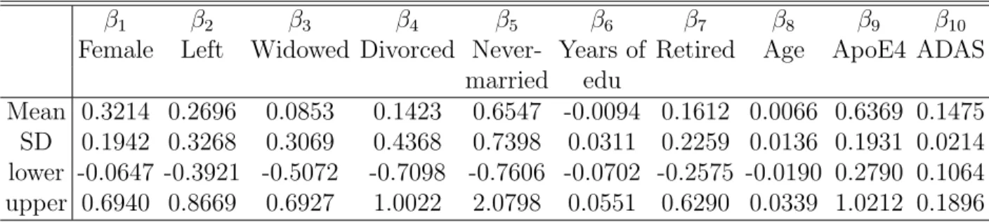
Table 3.1: ADNI data analysis results for the full BFLCRM model: the posterior quantities of 19 regression coefficients βks, that correspond to xi =(Gender, Handedness, Widowed,
Divorced, Never married, Length of Education, Retirement, Age, APOE-4 carrier, ADAS-cog Score, posterior limb of internal capsule, Right hippocampal formation, Left hippocampal formation, Left thalamus, Left amygdala, Right amygdala, and Right thalamus). Mean denotes ‘posterior mean’, SD denotes ‘posterior standard deviation’, and lower and upper, respectively, represent the ‘lower and upper limits’ of a 95% highest posterior density interval.
β1 β2 β3 β4 β5 β6 β7 β8
Female Left Widowed Divorced Never- Years of Retired Age married education in years Mean 0.4344 0.2255 0.3119 0.2729 0.7203 -0.0874 0.3455 -0.0519 SD 0.2513 0.3647 0.3827 0.4663 0.7867 0.0367 0.2482 0.0178 lower -0.0495 -0.5248 -0.4632 -0.6789 -0.9383 -0.1691 -0.0919 -0.0873 upper 0.9478 0.8628 1.0138 1.1195 2.2009 -0.0244 0.8608 -0.0188
β9 β10 β11 β12 β13 β14 β15 β16 β17
ApoE4 ADAS PLIC RHF LHF LT LA RA RT
Mean 0.5550 0.1568 0.0008 0.0006 -0.0011 -0.0004 0.0018 -0.0012 0.0003 SD 0.2341 0.0265 0.0005 0.0004 0.0004 0.0004 0.0009 0.0005 0.0004 lower 0.1258 0.1030 -0.0002 -0.0002 -0.0019 -0.0012 0.0000 -0.0023 -0.0004 upper 1.0258 0.2075 0.0019 0.0014 -0.0004 0.0003 0.0036 -0.0002 0.0010
(a) Top (b) Bottom
positive
negative
(c) Color bar
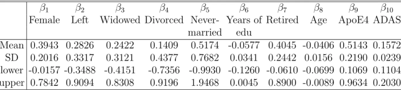
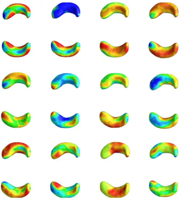
Figure 3.2: ADNI data analysis results for the full BFLCRM model: panels (a) and (b), respectively, show the top and bottom views of the estimated coefficient function associated with the hippocampal surface data color-coded by the colorbar in panel (c).
We estimated the coefficient function γ(·) by using ˆγ(s) = P14
j=1φˆj(s)ˆγj, where ˆγj is the posterior mean of γj for each j. Figure 3.2 shows the estimated coefficient function ˆγ(·)
associated with the hippocampal surface data. When hippocampal atrophy in a red region is greater, a risk of progressing from MCI to AD is expected to be increased. A blue region suggests that the thicker the area is on the hippocampus, the shorter the time to conversion to AD is. Inspecting Figure 3.2 reveals that the subfields of CA1 and subiculum on the hippocampi have positive effects on the hazard function, indicating that the thinner these areas on the hippocampus are, the shorter the time is to conversion to AD.
Figure 3.3 on page 31 shows the estimated survival functions of the APOE-4 carriers and non-carriers, when the values of the continuous covariates are set at their mean values and the categorical variables are set at their reference levels. The dotted lines show the 95% HPD intervals of survival functions. The APOE-4 carriers are expected to convert from MCI to AD faster than non-carriers. These results are consistent with several prior studies suggesting that the presence of the APOE-4 allele increases the risk of developing AD [148, 135, 27].
500 1000 1500
0.0
0.2
0.4
0.6
0.8
1.0
Time (days)
Su
rvi
va
l f
un
ct
io
n
95% HPD intervals for
Carriers
Non-carriers
Carriers
Non-carriers
Figure 3.3: ADNI data analysis results: the estimated survival curves of APOE-4 carriers and non-carriers under the full BFLCRM model. Other continuous or categorical covariates are fixed at the mean values or reference levels. The dotted lines show the 95% HPD intervals of the estimated survival functions.
predictive performance. For Model 1, we excluded the ROI volume covariates from the full BFLCRM model. For Model 2, we only included all the scalar covariates. For Model 3, we only included the clinical covariates, APOE-4 status, and the ADAS-cog score. For all three reduced models, we set J = 70 intervals so that each interval contains at least one failure or censored observation. For the regression coefficients, the hyperparameters of the multivariate Normal priors were set as µ0 = (0,· · · ,0) and Σ0 = diag(5,· · · ,5). We set
α0j = 0.2 and α1j = 0.4 for j = 1,· · ·,70. We ran the Gibbs sampler for 25,000 iterations
Table 3.2: ADNI data analysis results under the four models: DICs and the empirical means of iAUC values and their corresponding standard errors in the parenthesis calculated from the Monte Carlo cross-validation (MCCV).
the full BFLCRM model Model 1 Model 2 Model 3
DIC 427.19 413.08 417.04 438.22
iAUC 0.840 (0.003) 0.836 (0.003) 0.809 (0.003) 0.751 (0.004)
Table 3.3: ADNI data analysis results for Model 1: the posterior quantities of 12 regression coefficients βks, that correspond to xi =(Gender, Handedness, Widowed, Divorced, Never
married, Length of Education, Retirement, Age, APOE-4 carrier, and ADAS-cog Score). Mean denotes ‘posterior mean’, SD denotes ‘posterior standard deviation’, and lower and upper, respectively, represent the ‘lower and upper limits’ of a 95% highest posterior density interval.
β1 β2 β3 β4 β5 β6 β7 β8 β9 β10
Female Left Widowed Divorced Never- Years of Retired Age ApoE4 ADAS married edu
Mean 0.3943 0.2826 0.2422 0.1409 0.5174 -0.0577 0.4045 -0.0406 0.5143 0.1572 SD 0.2016 0.3317 0.3121 0.4377 0.7682 0.0341 0.2442 0.0156 0.2190 0.0239 lower -0.0157 -0.3488 -0.4151 -0.7356 -0.9930 -0.1260 -0.0610 -0.0699 0.1069 0.1104 upper 0.7842 0.9094 0.8308 0.9196 1.9468 0.0045 0.8900 -0.0089 0.9634 0.2030
found in [146, 76].
200 subjects and a test set with 146 subjects. For each such split, we fitted each model to the training set and then calculated iAUC based on the test set. This random split was repeated 100 times yielding the estimated iAUC values for all models.
3.3.5 Sensitivity Analysis
We examine the effects of varying hyperparameters on the posterior estimation. In our main paper, we first set p(β,γ,λ) = p(β,γ)p(λ) and assume (β,γ) ∼ N(µ0,Σ0), where
N(µ0,Σ0) is the multivariate normal distribution with a (p+qn)×1 mean vector µ0 and a (p+qn)×(p+qn) covariance matrix Σ0. For the piecewise constant baseline hazard function, λ = (λ1,· · · , λJ)T follows the independent gamma prior such that the λj are independent
and λj ∼ G(α0j, α1j) for j = 1, . . . , J, where α0j and α1j are prior hyperparameters. We
consider different choices of Σ0 and (α0j, α1j) and evaluate their effects on the estimation of
(β,γ,λ).
First, we varied the hyperparameter Σ0, while fixing (α0j, α1j) at (0.2, 0.4) for all j = 1,· · · ,70 . The mean vector µ0 was set as (0,· · · ,0) in order to reflect an in-sufficient prior information. For the covariance matrix Σ0, we considered three scenar-ios including diag(5,· · · ,5), diag(25,· · · ,25), and diag(100,· · · ,100). Particularly, Σ0 = diag(100,· · · ,100) represents an approximately non-informative prior. Tables 3.11 and 3.13 show that all posterior estimates are quite stable as Σ0 is varied.
Second, we varied the hyperparameters of the gamma priors on the piecewise constant baseline hazard function, when µ0 and Σ0 were, respectively, set to be (0,· · · ,0) and diag(100,· · · ,100). We considered three scenarios. To use non-informative priors forλj’s, we
set the shape and scale parameters of the gamma distributions to beα0j = 0.2 andα1j = 0.4
for all j = 1,· · · ,70 [143]. We then set either (α0j, α1j) = (0.2,1) or (α0j, α1j) = (0.5,1) in
50 estimated λj’s. Tables 3.12 and 3.14 show that all posterior estimates are quite stable as
the hyper parameters (α0j, α1j) vary. Therefore, we may conclude that the proposed priors
for a large range of hyper-parameters can yield stable posterior estimates.
3.4 Simulation Studies
We conduct Monte Carlo simulations to evaluate the proposed BFLCRM across differ-ent censoring rates and sample sizes. Moreover, we will evaluate the predictability of our BFLCRM compared to proportional hazards models without the use of functional covariates.
3.4.1 Setup
We generated all simulated data sets according to model (3.2.1). The xi is a 4×1 vector
and its corresponding elements were independently generated from N(0,0.5). We set the true value ofβto be (0.7,0.2,−0.5,−1)T. The functional covariateZi(s) was generated from
model (3.2.3), where its underlying function follows the standard Gaussian process with the covariance functionK(s, t) = exp(−3(s−t)2). The observed functional covariate dataW
i(s)
consists of noisy observations evaluated at 100 equally spaced grids in the interval [-4,4] with some measurement errors. Specifically, the measurement errors i(s) were independently
generated from a N(0,0.5) across s. The functional coefficientγ(s) was generated from the standard Gaussian process with covariance function Kγ(s, t) = exp(−2(s−t)2). To generate
the survival time, we considered two different baseline hazard functions h01(·) and h02(·) as follows.
h01(t) = 1 if t >0, (3.4.1)
h02(t) =
κω if 0< t≤2;
κω(t−1)ω−1 if 2< t≤3;
κω2ω−1 if t >3.
The first baseline hazard functionh01(·) assumes that it is constant over time. As a more general form of hazard function, we consider a mixed form of baseline hazard functions for the exponential and Weibull distributions. The hazard function h02(·) depends on κ and
ω. In this simulation study, we set κ = 1/3 and ω = 2. Finally, the censoring times were independently generated from a uniform distribution with parameter chosen to achieve a desired censoring rate of 30% or 50%. We considered sample sizes of n = 200 and n = 500 for each censoring rate and simulated 100 data sets for each case.
3.4.2 Simulation Results
We used the piecewise constant hazard model forh0(s), in which we setJ = 5 and subin-tervals (sj−1, sj] so that each interval contains at least one failure or censored observation.
We set (α0j, α1j) = (0.2,0.4) for all j, Σ0 = diag(5,· · · ,5), and µ0 = (0,· · · ,0)T. We cal-culated the first 12 fPC scores explaining 95% of the variation of the functional covariates, and then compared the estimation results using the first 12 PC scores in order to investigate the efficacy of using fPCA. For each simulated data set, we ran the Gibbs sampler for 20,000 iterations with 5,000 burn-in iterations.
To examine the estimation and prediction performance of BFLCRM, we calculated mean squared errors (MSEs) and time-dependent integrated area under the curve (iAUC) [74] based on 100 simulated data sets for each scenario. The computational time (in C/C++ using an 8-cores 2.80 GHz Intel processor) was 50.3 seconds for BFLCRM with sample size 200 for one repetition. We let ˆβ denote the posterior mean of β. The MSE of ˆβ is defined by MSEβˆ =
Pp
j=1( ˆβj −β)
2, whereas the MSE for γ(·) is defined by MSE ˆ
γ =
R4
−4{ˆγ(s)−γ(s)}
2ds, where ˆ
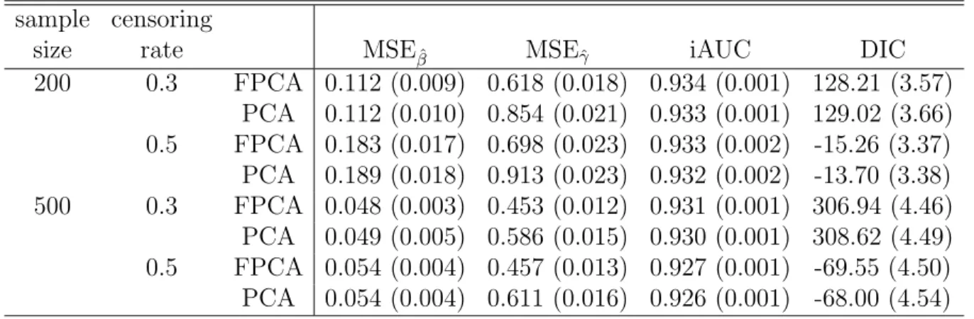
Table 3.4: Simulation results corresponding to h01(·) under different censoring rates and sample sizes: the deviance information criterion (DIC), the mean squared errors (MSE) of ˆβ and ˆγ and the estimated integrated area under the curve (iAUCs) and their standard errors in parentheses calculated from the 100 simulated data sets. The Gibbs sampler was run for 20,000 iterations with 5,000 burn-in iterations for each simulated data set.
sample censoring
size rate MSEβˆ MSEˆγ iAUC DIC
200 0.3 FPCA 0.109 (0.009) 0.614 (0.016) 0.935 (0.001) 42.99 (3.46) PCA 0.113 (0.010) 0.847 (0.020) 0.934 (0.001) 44.66 (3.58) 0.5 FPCA 0.181 (0.014) 0.696 (0.021) 0.933 (0.002) -93.80 (3.44)
PCA 0.186 (0.014) 0.913 (0.025) 0.932 (0.002) -92.21 (3.46) 500 0.3 FPCA 0.045 (0.003) 0.445 (0.012) 0.932 (0.001) 83.52 (4.52)
PCA 0.047 (0.003) 0.581 (0.015) 0.930 (0.001) 85.50 (4.57) 0.5 FPCA 0.052 (0.004) 0.454 (0.013) 0.928 (0.001) -260.93 (4.58)
PCA 0.052 (0.004) 0.600 (0.015) 0.927 (0.001) -259.37 (4.63) Table 3.5: Simulation results corresponding to h01(·): the mean iAUC and the correspond-ing standard error in the parenthesis calculated from the 100 simulated data sets for each scenario. The Gibbs sampler was run for 20,000 iterations with 5,000 burn-in iterations for each simulated data set.
n 200 500
Censoring rate 0.3 0.5 0.3 0.5
reduced 0.675 (0.004) 0.612 (0.006) 0.668 (0.002) 0.666 (0.002) full 0.935 (0.001) 0.933 (0.002) 0.932 (0.001) 0.928 (0.001)
and a full BFLCRM model with both Wi(·) and xi.
0 2 4 6 8 10 0.0 0.5 1.0 1.5 2.0
Time to event
Ba se lin e ha za rd fu nct io n True Estimated
(a) Censoring rate=0.3
0 2 4 6 8 10
0.0
0.5
1.0
1.5
2.0
Time to event
Ba se lin e ha za rd fu nct io n True Estimated
(b) Censoring rate=0.5
Figure 3.4: Simulation results corresponding to h01(·): panels (a) and (b) respectively show the first 10 estimated baseline hazard functions with 0.3 and 0.5 censoring rates based on the size 500 samples. The solid line is the true baseline hazard function, h01(·).
BFLCRM model is generally larger than that of the reduced model in all scenarios. This may indicate that the use of functional covariates can improve predictability of the hazard function. Figure 3.4 shows the baseline hazard functions estimated by the full BFLCRM from the first 10 data sets in the sample size 500 cases. The dotted lines show the estimated baseline hazard functions, and the true baseline hazard function h01(·) is plotted as a solid line on each plot. When the true baseline hazard function is constant, our model estimates the true function well in low to moderate censoring cases.