Labor Contracts, Equal Treatment and
Wage-Unemployment Dynamics
Abstract
This paper analyses a model in which …rms cannot pay discriminate based on year of entry to a …rm, and develops an equilibrium model of wage dynamics and unem-ployment. The model is developed under the assumption of worker mobility, so that workers can costlessly quit jobs at any time. Firms on the other hand are committed to contracts. Thus the model is related to Beaudry and DiNardo (1991). We solve for the dynamics of wages and unemployment, and show that real wages do not neces-sarily clear the labor market. Using sectoral productivity data from the post-war US economy, we assess the ability of the model to match actual unemployment and wage series. We also show that equal treatment follows in our model from the assumption of at-will employment contracting.
1
Introduction
This paper develops a model in which …rms cannot pay discriminate based on year of entry to a …rm— there are no “cohort e¤ects”— and develops an equilibrium model of wage dynamics and unemployment. The model is developed under the assumption of worker risk aversion, and also mobility, so that workers can costlessly quit jobs at any time. Firms on the other hand are risk neutral and are committed to contracts. Firms have to trade-o¤ the desire to insure their risk-averse workers against the need to respond to market conditions to not only prevent their workers from quitting but, because of equal treatment of workers, also to take advantage of states of the world where labor is cheap. We solve for the dynamics of wages and unemployment when the only exogenous variable is productivity shocks, and show that real wages exhibit a downward stickiness, due to the desire to insure incumbent workers. The equal treatment assumption prevents …rms from cutting wages for new entrants, so that in periods with adverse shocks the wage may not fall su¢ ciently to clear the labor market. We argue that even our rudimentary model, when fed sectoral productivity shocks from the post-war U.S. economy, gives a reasonably good account of unemployment and wage movements.
The idea that internal equity considerations can play a part in wage rigidity is by no means novel. Truman Bewley has argued recently that it is a key feature constraining wage cuts for new hires in recessions. In his story, because wage cuts for incumbents will have such a negative impact on morale, …rms avoid them under all but extreme circumstance; at the same time while new hires may be willing to work at a lower wage than that paid to incumbents, paying them less would disrupt internal equity and so their wages will be set at the same level as incumbents’(controlling for experience, etc.):
New employees, in contrast, feel it is inequitable to be paid according to a scale lower than the one that applied to colleagues that were hired earlier. For this reason, downward pay rigidity for new hires exists only because the pay
of existing employees is rigid. (Bewley (1999a))
Bringing in workers at higher pay than incumbents is even more problematic; thus while— in contrast to the primary sector— he found evidence that new hires are sometimes paid a lower rate than incumbents in the secondary sector, even there, paying new hires
more than incumbents is deemed to be very disruptive (Bewley (1999b, p. 320)).
Bewley’s account mainly concentrates on the question of why …rms do not cut wages in recession. But it raises the important question, which we attempt to answer, of how forward looking …rms take into account the fact that such constraints may arise in the future: for example, a …rm, anticipating this downward wage rigidity, may temper wage increases in better times. Or in more generality, and supposing that …rms can o¤er long-term contracts, the …rm must take into account these equal treatment constraints which will prevent it bringing in new hires at a low wage in downturns, and also prevent the …rm hiring at a higher wage than that o¤ered to incumbents when the labor market is tight. To our knowledge, the dynamic implications of equal treatment have not been analyzed elsewhere.1
The linking of the pay of new hires to that of incumbents means that wage rigidity also has real allocational implications. Obviously wage rigidity for incumbents need not imply deviations from Arrow-Debreu outcomes so long as hiring is at the e¢ cient level (in our model workers only separate for exogenous reasons). We show however that (under certain conditions) …rms hire up to the point where the real wage equals the marginal product of labor; to the extent then that wages do not correspond to market-clearing levels hiring will be ine¢ cient; in fact we show that this occurs only in the direction of wages being too high leading to ine¢ ciently low employment and an excess supply of labor.
1Our model di¤ers from Bewley’s account in that the motive to temper incumbent wage cuts arises
from to the desire to insure workers, rather than directly from worker morale considerations. We do not view this contracting perspective to be necessarily inconsistent with his account however. The morale e¤ects due to wage cuts that he documents might be considered to be the response by the workforce to a perception that the …rm has violated an implicit insurance contract: low worker morale might be regarded as a punishment mechanism used to sustain the implicit contract.
The paper builds on the seminal contribution of Beaudry and DiNardo (1991) (here-after BD). They develop a model of labor contracting where a risk-neutral …rm o¤ers insurance to risk-averse employees but, following Holmstrom (1983), there is no worker commitment (perfect mobility). Wages follow a ratchet-like process, rising when produc-tivity is higher than previously, but staying constant otherwise; they show that the current wage is determined by the tightest labor market during a worker’s tenure. In testing, this perfect mobility model does better than two alternatives: a spot market model in which current unemployment determines wages, and a full commitment model in which unem-ployment at the time of hiring is the determining factor. Subsequent research (McDonald and Worswick 1999, Grant 2003, Shin and Shin 2003, Devereux and Hart 2005) has largely con…rmed these results over di¤erent periods and using di¤erent datasets, although both Grant, and Devereux and Hart, …nd more of a role for the current unemployment rate than did BD. Although the economic environments are distinct, in essence our theoretical model deviates from theirs only in the imposition of equal treatment.
In BD, without the equal treatment assumption, each worker is treated independently, and the partial equilibrium analysis then boils down to a two-player game in which com-petition forces pro…ts to zero (given their constant returns to scale technology). It follows that the labor market must always clear, since at the point of hiring there are no restric-tions on wages. The downward wage rigidity in their perfect mobility model provides insurance to the worker but does not directly a¤ect employment decisions. Here, by con-trast, we do not allow …rms to treat each worker separately, but each new cohort of hires must …t into an existing wage structure. Even though we …nd that the characterization of optimal contracts is in a number of respects similar to that in BD, the implications for employment are very di¤erent, as there will be episodes of involuntary unemployment. We also show that although very robust, the estimated business cycle e¤ect on wages (i.e., through the minimum unemployment rate) in their estimations cannot explain very much of the movement of wages over the sample we look at (an extension of the one they
examine). On the other hand, wage movements predicted by our model can explain much of this.
The idea that equal treatment can lead to wage rigidity has been argued in a union context by Carruth and Oswald (1987) and Gottfries (1992). In these papers, outsiders have reservation wages below any wage that insiders might receive even in “good” states of the world. Wages are kept constant in the face of rising demand to prevent too much surplus leaking to outsiders. More closely related, Thomas (2005) considers an essentially static model with risk neutral workers and unveri…able states; in combination with equal treatment this can lead to wage-stickinessacross states in a given period (but not as here, over time).
There is little direct empirical evidence on the issue of equal treatment. The principal exception is a study of pay discrimination by Baker, Gibbs and Holmstrom (1994), who examined the pay of managerial employees in a single …rm over time. They found that incumbents’ pay tends to move together, but the pay of entrants is signi…cantly more variable, suggesting that the pay of new hires may be more subject to outside conditions than that of incumbents. However, as discussed above, survey evidence in Bewley (1999b) suggests that violations of equal treatment are unusual, particularly in the primary sector. Similar …ndings exist for other countries: “Managers responded that hiring underbidders would violate their internal wage policy” (Agell and Lundborg (1999, p.7), based on a Swedish survey); in a British survey, Kaufman (1984) reported that almost all managers viewed bringing in similarly quali…ed workers at lower wage rates as “infeasible.” Akerlof and Yellen (1990) argue that personnel management texts treat the need for equitable pay as virtually self-evident.
It is possible to derive some version of equal treatment from primitive hypotheses. For example, Moore (1983) shows that if it is necessary to retain at least one worker to train the new employees, then there is a unique von Neumann-Morgernstern stable
set consisting of con…gurations in which all workers receive the same wage. We adopt a similar approach using the idea that pay di¤erences may be exploited by employers to replace more expensive workers by cheaper ones, and that it is di¢ cult to distinguish between voluntary quits and …res, or alternatively, labor law requires contracts to be “at will”, so either party can dissolve the relationship without penalty (but, crucially, not vary the wage).
An outline of the paper is as follows. The model is presented and solved in Section 2. In 2.3 we show that equal treatment arises in equilibrium if labor contracts are “at will.” Empirical evidence is considered in Section 3: in 3.1 we outline our strategy for using sectoral TFP data from the postwar US economy to simulate the model and generate predictions of unemployment movements; in 3.2 we argue that a simulated wage from our model gives a reasonable account for macroeconomic wage movements, and although we con…rm BD’s …ndings over a longer sample than they study, their approach cannot account for aggregate wage ‡uctuations. Finally Section 4 contains concluding comments.
2
The model
The model is as follows. There is a horizon T,t= 1;2;3: : : T, whereT 2 may be …nite or in…nite, and a single consumption good each period. All workers are assumed to be identical, apart from the date of entry into the economy (we abstract from any tenure or experience e¤ects on productivity). Workers are risk averse with per period twice di¤erentiable utility function u(w); u0 > 0; u00 < 0; where w is the income/consumption received within the period; it is assumed that they cannot make credit market transactions. There is no disutility of work, but hours are …xed so that workers are either employed or unemployed. Assume that if workers are not employed in a period, they receive some low consumption levelc 0:There is a large (but …xed) number of identical risk-neutral …rms. The …rm has a diminishing returns technology where output is f(N; st) with @f =@N > 0; @2f =@N2 <0;whereN is labor input andstis the current productivity shock (the sole
source of ‡uctuations). It is assumed that a …rm must always employ some (minimum measure of) workers each period.2 Workers and …rms discount the future with respective factors w; f 2(0;1):There is an exogenous separation probability of(1 ), 2(0;1); each period, and separated workers must seek work elsewhere. Separation occurs at the end of a period so that separated workers who …nd a job in the following period do not su¤er unemployment. Moreover, there are a large number of workers relative to the number of …rms, and we normalize the ratio of workers to …rms to be one each period.3 We assume that the “spot wage”solution is always greater than the unemployment consumption level: @F=@N(1; st)> c all t:
The state of nature (productivity) st follows a Markov process, with initial value
s1; and countable state space S, but assume that from any state s only a …nite number
of states r 2 S are reachable next period with transition probabilities: sr > 0.4 Let
ht (s1; s2; : : : ; st) be the history att. While the …rm is committed to contracts, workers
are not (although we relax this later). The labor market o¤ers a worker currently looking for work (at the start oft) a utility (discounted tot) of t= (ht). We assume symmetry
between the situation of a worker who is currently employed and one who is searching for work, by assuming that a worker who either is separated from, or quits, their current employer attgets (ht). Thus a …rm must o¤er at least (ht)to prevent its workers from
quitting, and this is also the minimum utility that must be o¤ered to hire: We assume that the …rm can hire any number of workers by o¤ering at least t (and cannot hire otherwise). So the labor market is modelled as being competitive.
Our strategy will be to construct an equilibrium under the working hypothesis that …rms hire each period (so they replace at least some of those who are separated), and then
2
This can be motivated by an assumption that …rms cannot produce after a period of zero production.
3
Thus we take the fraction of a …rm’s workforce leaving to be exactly (1 ). IfN was …nite, then the fraction leaving a …rm would be random, and it can be shown that the contract could be improved by conditioning on this. (An alternative assumption to N large would be to simply rule out contracts that condition on this fraction on the grounds that veri…cation may be impossible.)
4
We use a Markov process to …x ideas, although the arguments go through for more general stochastic processes.
later we will …nd a restriction on parameters under which hiring does indeed always occur. This working hypothesis will also imply that we can ignore layo¤s, but formally we will state the optimization problemimposing no layo¤s, to avoid complicating the statement of the problem. Then we shall construct the hiring equilibrium as a solution to this problem. Finally it will follow that the hiring equilibrium is also a solution to a problem in which layo¤s are permitted.5
We work with a representative …rm, and we shall use a superscript to denote equi-librium values. At the start of date 1; after s1 is observed, …rms commit to contracts
(wt(ht))Tt=1 = (w1(h1); w2(h2); w3(h3); : : :),wt(ht) 0, which we assume are not binding
on workers. We assume equal treatment: a worker joining subsequently, at after history h , is o¤ered a continuation of this same contract: (w (h ); w +1(h ; s +1);w +2(h ; s +1;
s +2); : : :). (This is to be contrasted with the case where discrimination is permitted: in
that case a worker joining at is o¤ered a contract which in principle may be unrelated to that o¤ered to previous cohorts.) Let Vt(ht) denote the continuation utility from t
onwards from the contract:
Vt(ht) = u(wt(ht)) + (1) E " T X t0=t+1 ( w)t0 th t0 tu(wt0(ht0)) + t 0 t 1 (1 ) t0 i jht # ;
whereEdenotes expectation, and the term involving t0 re‡ects the utility after exogenous
separation. Each …rm also has a planned employment path(Nt(ht))Tt=1, whereNt(ht) 0:
The problem faced by the …rm is:
max (wt(ht))Tt=1;(Nt(ht))Tt=1 E " T X t=1 ( f)t 1(f(Nt(ht)) Nt(ht)wt(ht)) # (Problem A) subject to Vt(ht) (ht) (2) 5
Thus given that the rate of separation is exogenous, movements in unemployment occur through changes in hiring. This is consistent with the evidence reviewed in Hall (2005) that shows that the separation rate is roughly constant. Although job losses rise during recessions, the increase is usually very small in relation to the normal levels of separations.
for all positive probabilityht; T t 1, and
Nt(ht 1; s) Nt 1(ht 1) (3)
for all positive probability ht 1; all s 2 S with st 1s > 0; T t 2. (2) is the
participation constraint that says that at any point in the future the contract must o¤er at least what a worker can get by quitting, while (3) imposes that the …rm may not layo¤ workers.6
The outside option is determined by the following in a symmetric equilibrium:
t=Nt(ht)Vt (ht) + (1 Nt(ht))Ut(ht) (4)
where Ut(ht) is the discounted utility of a worker who is unemployed at t, so Ut(ht) =
u(c) + wE t+1 jht ;i.e., the utility from the reservation wage plus future utility from
not having a job at the beginning of t+ 1.7 There are two cases: if the labor market at timetclears,Nt(ht) = 1, then from (4) it must o¤er the utility o¤ered by other …rms. In
symmetric equilibrium, other …rms are o¤ering an identical contract, and so it is the utility associated with this,Vt (ht);which must be o¤ered. If, on the other hand, there is excess
supply of labor,8 Nt(ht) < 1, the outside opportunity will depend on the probability of
getting a job, Nt(ht). (Recall that quitters, those exogenously separated at the end of
the previous period, and the unemployed from the previous period, are all in the same position.)
Necessary conditions for an optimal contract can be characterized with the help of a simple variational argument. This is the central idea explaining why there is a lower bound on the fall of real wages; even if the labor market is slack at t+ 1, the …rm will not want
6
More precisely, (3) implies layo¤s are notneeded. However the de…nition ofVt(ht)in (1) implies that a worker remains with the …rm unless exogenously separated, so together these two assumptions rule out layo¤s. We show in the Appendix that our solution is robust to allowing layo¤s.
7Clearly
t Ut(ht), since remaining unemployed is an option for workers (i.e., if Vt (ht) < Ut(ht) then no workers would accept jobs andNt(ht) = 0). So ifVt(ht) t;unemployed workers are not better o¤ refusing a job.
8
Intuitively, the case of excess demand for labour cannot arise in equilibrium, as an in…nitessimally small increase in the wage would cure the individual …rm’s supply problem. In contrast, because of equal treatment the case of excess supply can arise since workers cannot undercut.
to cut the wage too far because of the desire to insure incumbents. Once this point is reached, the wage will not fall faster no matter how low the supply price of outside workers (i.e., new hires will strictly want to work for the …rm in this case). Suppose we are at ht;
let Nt and Nts+1 denote the optimal employment levels after ht and (ht; s) respectively,
and consider, starting from the optimal contract, reshu- ing wages between t, and t+ 1
in state s; to backload them. Increase the wage at t+ 1 after states by a small amount ; and cut the wage at t by x so as to leave the worker indi¤erent; do not change the contract otherwise:
sts wu0(wt+1(ht; s)) u0(wt(ht))x'0:
This backloading satis…es all participation constraints since worker utility rises at t+ 1; and so from this point on constraints are satis…ed, but also afterhtand earlier since utility
is held constant over the two periods. The change in pro…ts (viewed fromht) is
sts fN s t+1 +Ntx' sts fN s t+1 + sts wu0(wt+1(ht; s))Nt u0(wt(ht)) ; which is positive for small enough unless
u0(wt+1(ht; s))
u0(wt(ht))
fNts+1
Nt w
: (5)
Since the change in pro…ts cannot be positive by optimality of the original contract, (5) must hold: marginal utility growth cannot exceed a certain amount. Conversely, the reverse argument (frontloading), which would be pro…table if the strict version of (5) holds, cannot be undertaken (only) if next period’s participation constraint binds since utility falls at t+ 1; so the constraint would be violated. We summarize the necessary condition:
Lemma 1 In an optimal contract with perfect mobility, (5) must hold; it can only hold strictly (<) if the participation constraint binds at(ht; s):
“target marginal utility growth rate”: u0(wt+1(ht; s)) u0(wt(ht)) = fNts+1 Nt w (6)
which will be maintained, unless a binding participation constraint att+ 1forces it to be lower. Put di¤erently, this puts a lower bound on how fast real wages can decline, but a tight labor market at t+ 1can imply that wage growth is not against this bound. Note that this lemma applies whether or not the …rm is hiring att ort+ 1.
It is instructive to compare this with the BD model (in this context) which has symmetric discounting, so assume that f = w. The corresponding target (gross) “growth rate” in their model is 1: wages stay constant unless a binding participation constraint forces them to be higher. The only di¤erence arises here because the term Nts+1=Nt
re‡ects the number of new hires that will be made next period for each incumbent at t. The reason is the following: if discrimination is allowed (as in BD) then each worker is treated independently, so the risk-neutral …rm would like to fully insure each worker by holding wages constant.9 In the equal treatment model, wages would likewise be constant if the term Ns
t+1=Nt = 1, that is, if none of the workers who separate are replaced. In
this case the …rm is only having to deal with the incumbents, so this corresponds to the discrimination case. Whenever Nts+1=Nt >1, however, the …rm is taking on additional
workers att+ 1who will receive the same wage as the incumbents; hence the future wage is taken into account with a larger weight by the …rm than by the incumbent worker, and this imparts a downward bias to the future wage in comparison with the discrimination case.
To proceed, assume provisionally that …rms always hire (at all ht) in equilibrium. That
is to say, we proceed on the supposition that the constraint (3) in problem A never binds in the solution. We characterize the solution if this is the case, and later …nd conditions on 9The exogenous separation probability a¤ects …rm and worker equally— the …rm only has to pay the
agreed upon wage next period with probability (times stst+1) and the worker only receives the wage with the same probability— so it nets out.
a speci…c parametrization for which the solution satis…es this property. Finally we verify that this is also a solution to the original problem.
Then employment is determined by a standard marginal productivity equation:
Lemma 2 If in a symmetric equilibrium hiring takes place at every ht; thenNt(ht) sat-is…es
@F(Nt(ht); st)=@N =wt(ht): (7)
Proof. Suppose that @F(Nt(ht); st)=@N > wt(ht): It is feasible to increase current
hiring holding the wage contract constant, and consider this as the only change to the …rm’s plan: An increase in current hiring by >0, for small enough, and holding the wage constant at wt(ht), would lead to an increase in current pro…ts. At the same time,
holding employment att+ 1constant atNt+1(ht+1)in all states (so hiring falls by ), is
feasible for small enough given hiring is positive at t+ 1. Thus there is an increase in pro…ts att;and no change at other dates, contradicting pro…t maximization. A symmetric argument, using the fact that current hiring is positive so current hiring can be reduced
by ; and that t+ 1 employment can be increased by , rules out @F(Nt(ht); st)=@N
< wt(ht):
Suppose that at some t; the participation constraint binds. Then there must be full employment and the wage is determined by marginal productivity at full employment:
Lemma 3 Consider a symmetric equilibrium in which hiring always occurs; then the par-ticipation constraint binds at htif and only ifNt(ht) = 1; moreover if the constraint binds then wt(ht) =@F(1; st)=@N:
Proof. (i) Suppose …rst that the participation constraint binds,
and suppose contrary to the lemma that Nt(ht) < 1: Under the hiring hypothesis, we
know from Lemma 2 that @F(Nt(ht); st)=@N =wt(ht) > c by the assumption on c and
diminishing marginal productivity (i.e.,wt(ht) cwould implyNt(ht)>1). Likewise, at
anyt0it is not possible thatw
t0(ht0) csince there is no feasible employment level (N 1)
for which @F(N; st)=@N c, and so Lemma 2 would be contradicted. Consequently, a
worker who gets a job at t receives strictly more current utility than the utility from being unemployed, and in the future receives no less no matter when (or if) she would get a job if unemployed today, given that she would receive w (h ) regardless of when she was hired; consequently an unemployed worker is strictly worse o¤ than an employed. Hence quitting at t will lead to a utility strictly less than Vt (ht) as there is a positive
probability of unemployment. This contradicts (8). The equilibrium wage follows directly from Lemma 2. (ii) Now suppose thatNt(ht) = 1:Since all workers are employed, t(ht)
is de…ned to be equal toVt (ht);so the participation constraint binds.
We de…ne ws = @F(1; s)=@N; which in view of the above lemma is the equilibrium wage when the participation constraint binds in state s. Then we can summarize: in a symmetric equilibrium with hiring, if at t+ 1 the participation constraint isn’t binding, wages are updated according to (6); if it is binding, then wt+1 =wst+1.
2.1 Empirical Implementation
To proceed to an explicit solution, in order to facilitate the empirical analysis, we put more structure on the problem.10 This will allow us to assert that the wage updating
rule is of the following simple form: given wt compute wt+1 under the hypothesis that
the participation constraint at t+ 1 is not binding; if wt+1 > wst+1 then the hypothesis is con…rmed and wt+1 is the equilibrium wage; otherwise the constraint is binding and
the equilibrium wage will be at wst+1. The structure will also allow us to demonstrate su¢ cient conditions for the symmetric hiring equilibrium to exist.
1 0Essentially we need the problem faced by the …rm to be concave; concave production and utility
From henceforth assume each …rm has technology given by, at timet,
F(N; st) =Mt+atN1 =(1 ); (9)
where > 0, 6= 1, Mt 0 and for < 1, Mt = 0. (Mt; at) will evolve according
to a Markov process, with f; w <min E[at+1=atjMt; at] 1; E[Mt+1=MtjMt; at] 1 .
Note that for > 1, F has an upper bound given by Mt, which given that we are
modelling short-run production functions at the establishment or plant level, may be appropriate. We also assume henceforth that workers have per-period utility functions of the constant relative risk aversion family with coe¢ cient > 0, 6= 1, described by u(c) =c1 =(1 ).11 Finally we assume that >1.
The “target” rate of wage growth (i.e., if unconstrained at t+ 1) is, from (6), wt+1 wt = Nt Nt+1 1 ; (10) where w
f . Under the hiring assumption, we also have that the marginal product of labor equals atNt , so that using (7),
Nt=a
1
t w
1
t : (11)
Combining (10) and (11) yields an equation for the evolution of wages if unconstrained at t+ 1 : wt+1 wt = 1 at+1 at 1 1 a t+1 at : (12)
where the function (:)simpli…es notation. Moreover if …rms are constrained att+ 1, then asNt+1 = 1,wt+1 =wst+1 =at+1 (from Lemma 3). We can now state
Proposition 4 In a symmetric equilibrium with positive hiring, wages will satisfy
wt+1 = max at+1
at
wt; at+1 ; (13)
where w1 =a1.
1 1For = 1, we can specifyF(N; s
Proof. We have just shown that wt+1 must equal one of the arguments of the max operator, depending on whether or not the participation constraint binds at t+ 1. Suppose …rst that at+1
at wt > at+1, which given > 1, can be rewritten as wt > at1at+1 1=( 1). Suppose that the participation constraint binds at t+ 1
(so wt+1 = at+1 and Nt+1 = 1) contrary to assertion. Lemma 1 implies that
wt+1 wt Nt
Nt+1 1
with equality unless the participation constraint binds att+ 1. Thusat+1=wt
a 1 t w 1 t =1 1=
, or equivalently wt at1at+1 1=( 1). So we have a contradic-tion. Alternatively, suppose that at+1
at wt < at+1, and suppose thatwt+1 =
at+1
at wt. But this implies that labor demand exceeds unity, which is incompatible with equilibrium. Finally if at+1
at wt = at+1; then whether the participation constraint either binds or does not, wt+1 equals this common value. To show that w1 =a1;note that in an optimal
contract the participation constraint binds at the initial date (t = 1): if it did not, the …rm would increase pro…ts by cutting w1(s1) holding the remainder of the contract …xed,
and would still satisfy all participation constraints. Thus by Lemma 3 Nt(ht) = 1, so
w1 =a1.
It should be stressed that (13) must hold in a symmetric equilibrium in which hiring always takes place; i.e., it is a necessary condition.
2.1.1 A Numerical Example
We present a two period example (t= 1;2). Suppose that f(N; at) = atLogN where at
is the state of productivity at time t; with a1 = 1;and a2 taking values1:1 and 0:9;each
with probability 0:5; so productivity growth is 10%. Workers have a utility function u(w) = w 1;and c= 0:7. Assume there is symmetric discounting and that the survival probability is 0:87.
A spot market solution w~t would solve @f(N; at)=@N = wt at N = 1 (full
employ-ment), so thatw~t=at. From the analysis below, the only di¤erence in the equilibrium with
i.e., the wage in the bad state at t= 2 does not fall su¢ ciently to clear the labor market. Employment is determined by the standard wage equal marginal productivity condition, so that there is employment of 0:93 in the bad state, i.e., an unemployment rate of 7%; but full employment in the good state (and in period 1). Any attempt to cutw2(0:9)will lead to an increase in overall wage costs because the need to compensate period1hires for the extra wage variability more than o¤sets the fact that period2hires would be cheaper.
2.2 Parameter values for which hiring equilibrium exists
Using the above solution, the condition for hiring to occur at t+ 1is Nt+1 =a 1 t+1w 1 t+1 > Nt = a 1 t w 1 t : (14)
When will the hiring condition (14) be satis…ed, and when does the model predict outcomes other than spot market ones? The hiring condition requiresa
1 t+1w 1 t+1 > a 1 t w 1 t ; if …rms
are constrained att+ 1thenN = 1and hiring is positive; if they are not, then (12) holds, and after simpli…cation the condition becomes
at+1 at > 1 1 = w f 1 : (15)
Consequently, provided (15) holds for all states reachable with positive probability from (any)atthat occurs with positive probability, the wage path, given by (13), with associated
employment levels given by (11), is an equilibrium. For w = f, condition (15) requires that the maximum rate of fall of productivity should be smaller than the exogenous turnover rate raised to the power of .
To see when outcomes di¤er from spot outcomes, starting from full employment in some state at, we need the wage to fall by less than the spot wage. Thus we need, using
wt=at;from (12) wt+1 = 1 at+1 at 1 1 at> at+1
which can be rewritten as
at+1
at
Since 1
< 1 (from > 1), (15) and (16) are compatible: there exist shocks at+1
at
su¢ ciently small (“bad”) that the contract wage does not fall enough to maintain full employment, but not su¢ ciently small that hiring falls to zero.
Although we have found a unique solution to the necessary conditions under the hiring assumption, we have not yet shown that if this solution satis…es (14), then this is su¢ cient for it to be an equilibrium. This is established in Appendix A. where we consider a relaxed version of the problem faced by a potential deviant …rm and show that this cannot improve on the putative equilibrium; it follows that a deviant cannot do better in a more constrained version.
2.3 Endogenizing the Equal Treatment Constraint
So far we have simply imposed equal treatment as a constraint. In the absence of this constraint, a …rm will o¤er a lower cost contract to new hires in bad states of the world than the continuation of incumbents’contracts. Suppose however that courts cannot distinguish between a voluntary quit and one that is enforced by the employer, for example by making working conditions unpleasant, or alternatively by dismissing workers on the basis of minor contract violations. Alternatively it may be that the law stipulates that employment contracts must be “at will”.12 Thus we assume that a worker’s contract speci…es wages over time, but either …rm or worker can terminate it at any point. Then the …rm will have an incentive to replace incumbents by cheaper new hires in bad states. Given that workers will anticipate this, it does not follow that the ability to pay discriminate is advantageous to …rms.
In Appendix B we show that if pay discrimination occurs, the e¤ect of a cohort being ousted by a cheaper one can be replicated by a contract in which the incumbent cohort is 1 2The doctrine of at-will employment recognises “that where an employment was for an inde…nite term,
an employer may discharge an employee ‘for good cause, for no cause, or even for cause morally wrong, without being thereby guilty of legal wrong’.” (Wisconsin Supreme Court, 1983).
retained but paid according to the continuation of the new hires’contract; since the new hires’ contract must satisfy the participation constraint, and since the incumbents who are ousted at tin this fashion will receive exactly t, the incumbents cannot be worse o¤. (New hires brought in at on a di¤erent contract than that of incumbents can be allocated a continuation of the latter contract.) In this manner a new contract satisfying equal treatment can be constructed which is at least as good as the original contract which does not satisfy equal treatment. Hence a …rm cannot su¤er bycommitting to equal treatment, and we can show that the solution to the model derived above remains an equilibrium in an environment with no equal treatment requirement but with at-will contracts.
A related argument has been made in the insider-outsider context by, amongst others, Gottfries (1992) (see also Carmichael (1983) and MacLeod and Malcomson (1989)).13 There is some evidence for this concern existing among incumbent workers when faced with the possibility of two-tier wages, see, e.g., Bewley (1999b, p. 146).
2.4 Worker Commitment
We assumed that workers are not committed to contracts, and hence it is the ex post mobility of workers which drives the wage dynamics. Suppose we drop the assumption that workers can costlessly quit the …rm, for example by assuming that there is a mobility cost su¤ered if a worker changes jobs. Because of equal treatment, very little changes. If there is a symmetric equilibrium with mobility costs in which …rms hire every period, then it must be identical to a symmetric hiring equilibrium with ex post mobility since the same participation constraint needs to be satis…ed each period— if the continuation contract o¤ers enough to hire a new worker, then it will also o¤er enough to prevent a worker from
1 3
Gottfries and Sjostrom (2000) allow the …rm to …x a termination payment for workers, payable irre-spective of who initiates termination, which in principle should allow outsiders to be brought in at lower pay without creating incentives for replacement of insiders; on the other hand it increases turnover as insiders are more willing to leave. It is shown that the turnover e¤ect may stop the …rm from o¤ering termination payments. A similar argument can be made here if we allow for on-the-job search (which does
not,per se,a¤ect our equilibrium) so that termination payments may induce incumbents who …nd a job
leaving. However the converse may not be true: an equilibrium with fully mobile workers may not be one with mobility costs. It may pay …rms to choose not to hire in some periods (to avoid increases in wages) and letVt(ht) fall below (ht). In the mobility case
a …rm doing this will lose its incumbent workers too, something by assumption it wants to avoid. The two caseswill coincide if however we additionally assumed that a …rm must always hire some workers to replace separated workers; this could be justi…ed if there are ‘key’workers who cannot be replaced by reallocating incumbents and new workers must be hired and trained in these jobs; hence the participation constraint must be satis…ed at each date.
3
Empirical Evidence
In this section we examine the evidence in support of our theory using both unbalanced panel data from the Panel Study on Income Dynamics (PSID) and macroeconomic data from the Bureau for Labor Statistics (BLS). We start by assessing the success of our theory in explaining unemployment. Then we use the PSID to assess the relative success of BD’s empirically successful contracting model and our own in explaining macroeconomic wage movements over the cycle.
3.1 Macroeconomic Evidence: US Postwar Unemployment
In this subsection we assess how well our model …ts US post war aggregate unemployment data from the BLS and the US Abstract of Statistics. In the one sector model studied above, unemployment falls to zero whenever the productivity shock is not too bad. Using a multisector model in which each sector is subject to idiosyncratic productivity shocks we will obtain more realistic unemployment levels because it is less likely that all labor markets will simultaneously clear; moreover when the aggregate productivity shock is positive, there will be more sectors with low unemployment and consequently aggregate employment is likely to be lower. Naturally this exercise depends on how well correlated
the sectoral shocks are.
In order to get some realistic predictions from our model, we use actual U.S. man-ufacturing industry multifactor productivity processes for 17 sectors plus a residual non manufacturing sector, as provided by the BLS and then aggregate the model’s predictions made for each of these sectors. This simultaneously …xes the degree of shock correlation, and also allows us to generate simulated unemployment and wage series which can be directly compared to the data. We make the extreme assumption that each sector is oth-erwise independent, so that the sectoral labor markets are completely segmented.14 As we
shall see, even though the model is lightly parametrized (two degrees of freedom for wages and three for unemployment), feeding it these sectoral shocks leads to unemployment and wage predictions that correspond reasonably well to the data.
As Proposition 4 makes clear, given knowledge of the model’s parameters, given an initial time period where there was full employment and given a TFP series it is possible to generate the sectoral “real wage” series that would be predicted by our theory. We note that we are able to solve the model on this basis because of the convenient property that the solution depends only on actual realizations of the random processes, and not on their distributions. It is then possible to derive the corresponding implications for unemployment (rates).
We generate separate predicted wage and unemployment series for 17 manufactur-ing sectors and one residual non manufacturmanufactur-ing ”sector”, and then aggregate usmanufactur-ing each sector’s employment shares. To implement our simulations we need to calibrate the rate of change in real wages when …rms are unconstrained (and productivity is unchanged), 1;and and , the parameters governing (relative) risk aversion and the curvature of the production function respectively. For the coe¢ cient of relative risk aversion, ;we 1 4We use this data as it is the only sectoral TFP series available for such a long time scale and collected
on a consistent basis; TFP data for other broad sectors such as services are only available from the early 70’s onwards. It is also extreme to assume that these sectors map exactly into genuinely distinct and separate labor markets. Nonetheless we work with what is available to us and accept that what we are able to do will be more of an indicative rather than rigorous empirical exercise.
use the value 1.2 which is in the standard range for simulations and for we use 1.4. This translates to a short-run elasticity of demand for labor of approximately -0.7. Estevão and Wilson (1998) analyzing BLS manufacturing data for a similar period that we study, found a short-run demand elasticity ranging between close to zero and -0.71 with aggregate data, and of between -0.5 and -0.89 at the 4-digit industry level for manufacturing.15 In fact the wage solution depends only on two composite parameters, and 1. Thus varying and but keeping their product constant does not a¤ect the solution for wages provided we hold 1 constant; the unemployment series will vary with 1= however, as this measures the elasticity of labor demand by which wt=at > 1 (i.e., the extent to
which wages are too high for market clearing) translates into unemployment. Thus a lower value for will magnify ‡uctuations in sectoral unemployment. We set 1 to be
0:98 (equivalently, :99), which will lead to a distribution (depending on productivity shocks) of real wage declines when the constraint is not binding centred around 2% per year.16;17 Individual predicted wage series were generated for each of the 17 two digit manufacturing sectors for which TFP data are available from the BLS and for the residual sector (whose TFP is constructed as the weighted di¤erence of total nonfarm business TFP and manufacturing TFP, all in logs). Treating each sector as a separate economy
1 5Hamermesh (1993) reports that a lower elasticity, around 0:3, is typical. 1 6
Elsby (2005) charts the distribution of real wage changes in the PSID over a relatively low in‡ation period (so surprise in‡ation is less likely to lead to unanticipated real wage falls), 1983-1992; real wage falls rarely exceed about 6%, with a spike around 2-4%. Given that the data includes displaced workers who will receive wage cuts in their new jobs, our choice of the upper end of this range seems reasonable. Likewise Christophides and Stengos (Apr 2003) …nd from Canadian wage contract data in the unionized sector that most real wage reductions in the 1990s were of the order of 1-2%.
1 7Alternatively we could calibrate this term by calibrating its constituent parts
f; w; ; and . Certainly, given that annual turnover in the PSID is as high as 30%, this is likely to lead to a lower value for 1, which in turn would make labor markets more likely to clear. On the other hand, a richer thory would be likely to lead to a number of o¤setting elements. First, plant turnover, from which we abstracted, would have the opposite e¤ect from worker turnover on the target wage change. Secondly, it may be that much of the observed turnover is intentional in the sense workers are planning to leave when an appropriate opportunity comes along (particularly in the secondary sector) and are unlikely to be retained even by an appropriate wage policy. Such turnover should not enter into the expression for target wage growth. It is actually only separations which areunanticipated by workers who are not in the above category which matters for determing the target wage growth. (This can be seen in an extreme case; suppose that 30% of the workforce plans to leave at the end of the current period, to be replaced, and the other 70% will stay if wages are as good as elsewhere. Then the wage would in fact stay constant— if f = w and assuming next period’s participation constraint does not bind— since both stayers and the …rm trade-o¤ marginal wage changes at the two dates equally. The relevant is one.)
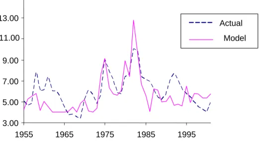
we used the model and the relevant TFP series to generate a simulated unemployment series for each sector. An aggregate unemployment index was then constructed as the weighted average of the individual sector simulations with weights given by employment shares.18 The results for actual aggregate unemployment and model unemployment are
graphed in Figure 1. The simulated model unemployment series appears to do quite well. In particular the volatility of actual unemployment is reasonably well matched as are the peaks and troughs of the actual series. Finally regressing actual unemployment (u) on the model predicted unemployment (bu) gives (standard errors in brackets):
ut = const+:734but R2=:42 t= 1955; : : : ;2001: (:128)
This con…rms what Figure 1 indicates, namely that there is a highly signi…cant rela-tionship between the actual and predicted series19. Finally as a robustness check on the correlation coe¢ cient between u and bu of 0:65; we allowed to vary between 0:98 and 0.995, ; between 1:1 and 2, and found that the correlation coe¢ cient varies between
0:59 and 0:66.
3.2 Macroeconomic Evidence from the PSID
We now assess the ability of the model’s predicted wage series— using the same calibra-tion as above— to explain movements in aggregate wages garnered from the PSID. One advantage of using the PSID for this purpose is that it was used by BD and this allows us to replicate their analysis (Appendix C con…rms their results on our longer sample) and assess the relative success of their key variable against our model prediction in explaining macro wage movements. Another advantage is that the aggregate annual wage we extract has been purged of the e¤ects of changes from year to year in worker characteristics. By 1 8The (…xed) employment weights were taken from the middle year of the sample and the manufacturing
sector as a whole was assumed to be 50% larger than the residual sector - roughly consistent with the average relative actual sizes over the period.
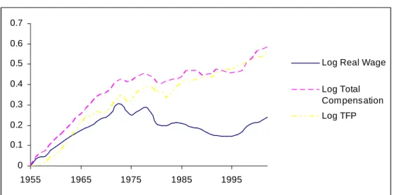
contrast the BLS aggregate wage series may move purely because of compositional changes of the working labor force over the business cycle. Given that our theory makes predic-tions for a representative individual the PSID panel is in many ways more appropriate benchmark target than is the BLS aggregate data.20 There is a problem with this however.
Our theory explains macroeconomic movements in wages purely in terms of productivity shocks. A glance at Figure 2 shows that between 1968 and 1993 real wages (non farm private sector) and aggregate TFP (likewise private nonfarm) have opposite trends— real wages fall whilst TFP rises— a general feature of postwar US data. But as is well known, there is an increasing discrepancy between total (wage plus nonwage) compensation and wages, due largely to sharp rises in company medical and pension, etc. bene…ts. If we look at total worker compensation (Figure 2 again) we see this clearly. Interestingly total compensation has roughly the same trend as TFP. In our model wages are driven largely by the demand for labor, which depends on total compensation not just its wage element. In what follows therefore we adjust annual real wage measures extracted from the PSID to allow for non wage compensation. As a …nal check on our empirical results we attempt to match the model’s wage predictions with wage estimates from the PSID allowing for di¤erent trends via detrending and as we shall see it does not substantially a¤ect our main results.
We collected data from the PSID for the years 1968 to 1993— encompassing the BD years of 1976-84. We collected data on private sector employees’hourly wage and a basic set of characteristics: gender, age, education, occupation, tenure (in months), race and state of residence. For the macro variates we use the annual CPI and monthly aggregate unemployment rates as reported by the BLS. Whilst we did not collect data on all of the BD characteristics21 we have arguably the most important and most frequently recorded ones. Unlike BD (but not Grant (2003)) we do not exclude women and individuals who
2 0
The BLS Employment Cost Index represents an attempt to measure year to year wage movements whilst controlling for changes in the year to year composition of the labour force. However this series starts relatively recently and a complete set of ECI …gures are unavailable for the years in our sample.
were in the workforce prior to 1947— this re‡ects our desire to be as comprehensive as possible in order to be able to generate macroeconomic results using the data later on.
The di¤erences in data collection make it impossible for us to replicate BD’s results exactly but we check whether the broad features of our sample are in line with theirs, and in Appendix C we report results con…rming their basic …ndings over our longer sample. Table 1 gives sample means and standard errors of our and BD’s main variates for the BD years. The table shows that we have nearly 30% more data points than do BD and that average wages in our sample are around 11% lower than in BD. Both of these di¤erences are largely though not wholly down to the inclusion of women (excluding women, for example, gives an average log wage less than 2% below BD’s). Average tenure is a little higher in BD but their key variable, minimum unemployment rate during job tenure (henceforth we refer to this variable as just “minu”) is rather lower than in our data. We should expect some di¤erences here as we did not adopt BD’s adjustment method. Instead we simply use the PSID variate “number of months with current employer” without adjustment.22
The predicted wage series for 1968-1993 from our model was an input into the analysis of unemployment undertaken above. (Recall that it was a weighted average of the model’s predicted wages for 17 manufacturing sectors and a residual sector.) To apply PSID data to our macro analysis we must do two things. First, because it reports wages not total compensation, some adjustment must be made when matching it with our simulated series. Second one has to take control for the e¤ect of the changes in yearly characteristics (e.g., the proportion of professionals in the year) which vary quite markedly over the sample years. We deal with the second issue …rst. We may write the following empirical model for PSID observations,wit:
wit = 0
cit+ meit+ mt+ 0
xt+"t+ it; (17)
wherewitare individuali’s log of wages de‡ated by the annual CPI in yeart(i= 1; :::nt), 2 2
For 1968 to 1974 the only tenure related question in the PSID refers to length of time in job rather than with employer which is somewhat ambiguous.
cit is a k 1 vector of individual i’s characteristics (6 occupation dummies, sex, 3 race
dummies, tenure, tenure squared, age, age squared, state of residence and 8 education dummies) at time t, xt is a vector of variables that have direct common in‡uence on
PSID wages (trend, cyclical variates, etc., to be speci…ed below) with = ( 1; 2:::) and
= ( 1; 2:::)being a conformable vector of parameters, andmeit=mit mtwithmitbeing
the BD measure of individual i0stightest labor market (i.e., the minimum unemployment rate) during his current job tenure at time t (“minu”) and mt being the sample mean of
mit in yeart.23 The errors"t= ("1; "2:::"T)and it = ( 11::: n11; 12::: n22::: 1T::: nTT)are assumed to be mean zero i:i:d. Taking annual averages of (17) gives the “macro” model for PSID wages as
wt= 0 ct+ mt+ 0 xt+"t+Op(nt1); (18) wherect= nt X i=1 cit
nt contains the annual means ofcit. In e¤ect this means that the only role of characteristics in the macro model is to allow for year to year compositional changes in the panel. If for example the 1968 data had a preponderance of professionals but the 1969 data was dominated by unskilled workers, we would expect a drop in wages that re‡ects a combination of the change in composition and the wage di¤erential between unskilled and professional workers. From the viewpoint of our macro theory we are really only interested in and in (18) because 0ctmerely picks up aggregate wage movements
associated with changes in the mix of characteristics in any particular year in the PSID. Explicitly we wish to analyse the relative importance ofmtand rival macro variables inx
such as trend, the simulated wages from our model and TFP. One obvious and direct way to do this would be to treat (18) as a simple regression (assuming that theOp(nt1)terms
are negligible) but there are two problems with this. First we have over 60 characteristics plus at least two further (macro) regressors but only 26 annual data points. Second, the left hand side variable wt excludes non wage bene…ts (pension, health insurance etc.)
which, from arguments given previously, are the relevant compensation measure in the 2 3
Constant terms are subsumed in the characteristic dummies and for simplicity are suppressed in the notation.
theory. The answer to the …rst conundrum is to exploit the cross section of the panel to obtain estimates of and to the second problem is to adjust wages for non wage bene…ts using aggregate data. We achieve these aims via two stage estimation. In the …rst stage we estimate (17) but allow mt+
0
xt+"tto be absorbed into year dummies. We therefore
estimate the model
wit= 0 cit+ meit+ T X t=1 tDt+ it; (19)
whereDt takes the value 1 in yeartbut zero otherwise.24 All of the macro e¤ects are now
captured in the estimates bt so that we can write
bt= mt+ 0
xt+"t+Op(nt1): (20)
To adjust for non wage bene…ts we add the BLS measure of the log of the ratio of aggregate total compensation to wages (rt) to the left hand side of (20), and denote this by bt
bt+rt.
There is reasonably strong evidence that bothbt and bt are trend stationary - ADF
statistics (with one augmentation) for the detrended series were borderline signi…cant for
bt at -3.41 and more robustly signi…cant for bt at -3.65 respectively when compared with
the critical value of -3.41. It is therefore reasonable to proceed under the trend stationarity assumption and estimate
bt bt+rt= mt+ 0
xt+"t+Op(nt1) (21)
free of restrictions. In particular we do not impose the restriction that the coe¢ cient on mtbe equal to in (19)— this allowsmtthe freedom to have a macroeconomic impact that
is separate from and unconstrained by its cross sectional/within year e¤ects on individual workers. Finally and again as a robustness check we also run versions of (21) withbtas the LHS variable. In BN’s model, mt explains bt (or bt) and in our model, because of equal
treatment, only the model predicted wage should matter once individual characteristics are controlled for.
2 4
Of course we may relax the i.i.d. assumption at this stage and allow for general forms of heteroscedas-ticity.
Figure 3 plots the detrended PSID estimates of total compensation (bdt) together with detrended macro minu (mdt) and detrended model predicted total compensation (wtd). Visual inspection suggests that the model’s predicted total compensation matches the dynamics of the PSID estimates rather better than does the macro measure of minu. More serious is the apparent positive association of mt with PSID total compensation
estimates which is perverse: larger values of the yearly averaged minushould imply lower total compensation in the year not higher.
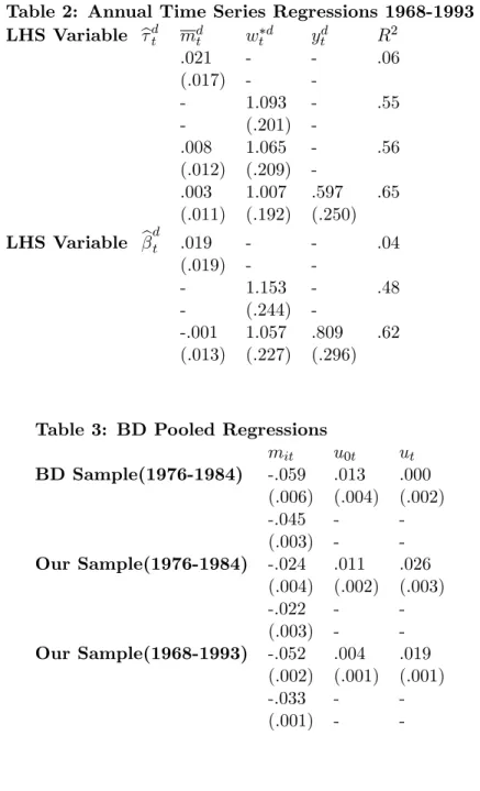
Table 2 gives regression results for a number of versions of (21). The regression of
bdt on mdt (…rst line) gives implausible results because themdt variable is insigni…cant and
incorrectly signed: the positive coe¢ cient implies that an increase in average minu from one year to another will lead to higher worker compensation, not lower as the theory would suggest. By contrast and turning to lines 3 to 6 of the table the two regressions of bdt on wtd and bdt on mdt and wtd show the model’s predicted series to be highly signi…cant in explaining total compensation estimated from the PSID. On its own, it captures 55% of the variation in bt compared with 6% for mdt and has a coe¢ cient very close to unity.
Adding detrended aggregate TFP (yd
t) to the regression (line 7) adds somewhat to the
explanatory power of the equation but not the size nor signi…cance of wtd. Althoughwtd is substantially more signi…cant than TFP, this regression does suggest that our model is some way from being a comprehensive explanation of the dynamic movements in total compensation— not surprising given the simplicity and parsimony of the model.
For completeness we report in lines 9 to 14 the regression of detrended PSID time e¤ects unadjusted for non-wage bene…ts (bdt) on mtd (line 9), onwtd(line 11) and on wtd andmdt (line 13). Overall the results are similar—wtdis important and robustly signi…cant whilstmdt is insigni…cant. In sum then our model predictions seem to track the dynamics of both PSID total compensation and PSID wage measures well.
thatminu is a statistically signi…cant determinant of individual wages (see Appendix C). Grant (2003) points out that its importance in accounting for the time series variation in wages may not be great because the variation in minu over time is not very large. If we add year dummies to a basic BD regression to absorb macro e¤ects (hence we regress log wages on characteristics, minu and year dummies) then we …nd, not surprisingly, that in both the short (BD) and long (68-93) samples minu explains less than 0.5% of the within year variation in log wages and accounts for less than 1% of the explained variance of wages in the pooled regression. More important from the macroeconomic viewpoint is minu’s contribution to the year by year/macro movements in log wages. Trend deviations in mean minuexplain only 3.8% of the variation in the trend deviations of log wages (see Table 2). It must of course be stressed that BD’s model is not formulated to explain macroeconomic phenomena, but to test alternative theories of contracting. Indeed, in cross section regressions, not reported in detail,minuremains signi…cant. Thus it appears successful in explaining di¤erentials between workers within a year, but it does not satisfactorily explain year to year movements in real wages.
4
Closing Comments
This paper has analyzed a model in which …rms cannot pay discriminate based on year of entry to a …rm. The trading-o¤ of wage insurance for incumbents against the desire to be ‡exible in the hiring wage paid to new hires leads to wages which do not always clear the labor market. On the other hand, the need to hire means that wages have to respond to su¢ ciently positive shocks, so that wages in the long-run respond to productivity move-ments. We …nd that these two features imply that the model gives a reasonable account of unemployment and compensation in recent US history.
References
Agell, Jonas and Per Lundborg, “Survey evidence on wage rigidity and unemploy-ment: Sweden in the 1990s,” June 1999. FIEF, University of Uppsala.
Akerlof, George A. and Janet L. Yellen, “The Fair Wage,”Quarterly Journal of Economics, 1990, 55, 255–283.
Baker, G., M. Gibbs, and B. Holmstrom, “The wage policy of a …rm,”Quarterly Journal of Economics, 1994,109, 921–955.
Beaudry, P. and J. DiNardo, “The E¤ect of Implicit Contracts on the Movement of Wages over the Business-cycle - Evidence from Micro Data,”Journal of Political Economy, 1991, 99, 665–688.
Bewley, T. F., “Work Motivation,”Federal reserve Bank of St. Louis Review, May/June 1999, 81(3), 35–50.
Bewley, Truman F., Why Wages Don’t Fall During a Recession, Harvard: Harvard University Press, 1999.
Carmichael, L., “Firm-speci…c human-capital and promotion ladders,”Bell Journal of Economics, 1983, 14, 251–258.
Carruth, A. A. and A. J. Oswald, “On union preferences and labormarket models -insiders and outsiders,”Economic Journal, 1987, 97, 431–445.
Christophides, Louis N. and Thanasis Stengos, “Wage rigidity in Canadian collec-tive bargaining agreements,”Industrial and Labor Relations Review, Apr 2003, 56
(3), 429–448.
Devereux, Paul J. and Robert A. Hart, “The Spot Market Matters: Evidence on Implicit Contracts from Britain,”IZA Discussion Papers 1497, Institute for the Study of Labor (IZA) February 2005.
Elsby, Michael W. L., “Evaluating the Economic Signi…cance of Downward Nominal Wage Rigidity: A Note on Nominal Wage Rigidity and Real Wage Cyclicality,” Dis-cussion Paper 704, Centre for Economic Performance 2005.
Estevão, Marcello M. and Beth Anne Wilson, “A Note on Nominal Wage Rigid-ity and Real Wage CyclicalRigid-ity,” Working Paper, Board of Governors of the Federal Reserve System April 1998.
Gottfries, N., “Insiders, outsiders, and nominal wage contracts,”Journal of Political Economy, 1992, 100, 252–270.
Gottfries, Nils and Tomas Sjostrom, “Insider Bargaining Power, Starting Wages, and Involuntary Unemployment,”Scandianvian Journal of Economics, April 2000, 102, 669–688.
Grant, Darren, “The E¤ect of Implicit Contracts on the Movement of wages over the Business Cycle: Evidence from National Longtitudinal Surveys,”Industrial and Labor Relations Review, April 2003,56(3), 393–408.
Hall, Robert E., “Job Loss, Job Finding, and Unemployment in the U.S. Economy over the Past Fifty Years,”NBER Macroeconomics Annual, 2005, pp. 101–137.
Hamermesh, Daniel,Labor Demand, Princeton: Princeton University Press, 1993.
Holmstrom, B., “Equilibrium long-term labor contracts,”Quarterly Journal of Eco-nomics, 1983, 98, 23–54.
Kaufman, R., “On Wage Stickiness in Britain’s Competitive Sector,”British Journal of Industrial Relations, 1984,22, 101–112.
MacLeod, W. B. and J. M. Malcomson, “Implicit contracts, incentive compatibility, and involuntary unemployment,”Econometrica, 1989,57, 447–480.
McDonald, James Ted and Christopher Worswick, “Wages, Implicit Contracts, and the Business Cycle: Evidence from Canadian Micro Data,”The Journal of Political Economy, Aug 1999, 107, 884–892.
Moore, John, “Stable Sets and Steady Wages,”April 1983. Birkbeck College, University of London.
Shin, Donggyun and Kwanho Shin, “Why are the wages of job stayers procyclical?,” March 2003. CIBC Working Paper No. 2003-7, The University of Western Ontario.
Thomas, Jonathan P., “Fair pay and a Wage-Bill Argument for low Real Wage Cycli-cality and Excessive Employment Variability,”Economic Journal, 2005, 115 (506), 833–859.
5
Appendix A: Su¢ ciency
Assume that the solution satisfying the necessary condition (13) satis…es (14) (recall that (15) guarantees this). We show that this is a solution to Problem A; moreover it is a solution to the problem where layo¤ s are permitted. We shall consider a relaxed version of the problem faced by a potential deviant …rm (i.e., where ( t)Tt=1 is …xed at the putative equilibrium levels) and show that this cannot improve on the putative equilibrium and use this to demonstrate that a deviant cannot do better in Problem A , nor when allows layo¤s are allowed. Layo¤ pay is ruled out for simplicity25 and we assume that a laid-o¤ worker receives t:
We deal with the caseT <1.26 We consider the problem as formulated earlier, but in which the …rm has no employment constraints, so that it solves Problem A without the constraint (3) (that is, it can costlessly reduce its workforce at any time, and only has to respect the participation constraints, which do not take into account layo¤s, this despite the fact that a worker in calculating his utility from the contract should take into account the layo¤ possibility). We call this Problem AR:We also consider the problem in which
layo¤s are permitted (these could be cohort dependent), but in which workers do factor in layo¤ probabilities into their calculations; this is the natural economic problem and we call it Problem B (for brevity’s sake we omit its statement).
Consider the static problem of maximizing pro…ts given that workers receive utility u, so that w = ((1 )u)1=(1 ). Substituting from (11) for N (this must hold in the static problem), yields pro…ts of
(u; at) Mt+ a 1 t ((1 )u) 1 (1 ) 1 : (22)
2 5Allowing for layo¤ pay raises the possibility that the …rm may want to replace its entire workforce in
bad states in order to bene…t from low outside wages. In the absence of layo¤ pay the incumbents will factor this into their calculations when deciding whether to join the …rm, and there can be no bene…t from this to the …rm (since an equivalent policy would be to retain the incumbents and to o¤er them a continuation utility of t). If the …rm could insure the incumbents it lays o¤, however, then the picture is less clear cut. Nevertheless, when a bad shock occurs, if the …rm is downsizing, as is likely to be the case, it cannot bene…t from replacing its workforce. Alternatively, we could introduce turnover costs which would render such a strategy unpro…table.
2 6
IfT =1, then by the assumption on f;we can show that pro…ts are …nite and standard arguments can be used to extend the …nite horizon argument.
As >1, this is a strictly concave function of u. We can formulate Problem AR faced by the …rm as: max (ut(ht))Tt=1 E " T X t=1 ( f)t 1 (ut(ht); at) # (Problem AR) subject to ~ Vt(ht) (ht) (23)
for all positive probabilityht; T t 1, where ~ Vt(ht) = ut(ht) + E " T X t0=t+1 ( w)t0 th t0 tut(ht0) + t0 t 1(1 ) t0 i jht # : (24)
Thus the maximand is strictly concave and the constraints are linear. The Slater condition is satis…ed by, for allht,ut(ht) =u(w (ht) +"), for" >0. Moreover it is straightforward
to show that the Kuhn-Tucker conditions are satis…ed at the putative equilibrium, hence the necessary conditions developed in the text are su¢ cient for existence in the relaxed problem.
Thus provided (14) holds, a solution to Problem AR exists and coincides with the solution to Problem A, and is the one we identi…ed. Consider now a feasible plan in Problem B which involves layo¤s occurring. Suppose we implement the same wage (i.e., utility) plan in Problem AR; (23) must hold given that any cohort facing a layo¤ probability in Problem B will get weakly less continuation utility than V~t:Since, givenwt;and hence
ut, per-period pro…ts are maximized in Problem AR;the solution to the latter must weakly
dominate the solution to Problem B. Putting this together, if (14) holds, our solution is also a solution to Problem B.
6
Appendix B: “At Will” Contracting Implies Equal
Treat-ment
We maintain the assumption that the …rm can commit to wages, which here includes commitment to the contracts of cohorts yet to be hired, but it cannot commit not to replace workers. We show that it is optimal to commit to a single wage policy, and that
our solution for the equal treatment case remains a solution with potential discrimination. For simplicity we treat the case of T …nite (although the argument can be extended to T =1):
Potentially a contract now will depend on the entry date to the …rm, so the wage at t of a cohort entering at t is denoted wt; with Nt the employment level at t; Nt(ht) Pt=1Nt(ht) now denotes aggregate employment at the …rm. We write a wage
contract as ! = (wt(ht)) t T
t=1, and an employment plan as = (Nt(ht)) t
T
t=1
where Nt+1 2 [0; Nt] for all t; t = 1; : : : ; T 1. We allow for layo¤s: a cohort worker who is still employed at t is forced to leave at t+ 1 with probability 1 Nt+1
Nt
for < t (this assumes no quits at t+ 1); this combines both the exogenous separation rate and any enforced terminations. Given(!; ),Vt (ht;!; )is the cohort’s continuation
utility from remaining with the …rm at t which takes into account the termination and quitting possibilities (we de…ne it for a worker att who willnot be laid o¤ nor quit att), de…ned recursively as:
Vt (ht;!; ) =u(wt) + wE
Nt+1
Nt maxfVt+1; t+1g+ 1
Nt+1
Nt t+1 jht ; (25) where VT+1; T+1 0: If Vt < t then the worker is better o¤ quitting at t.27 Vt is de…ned afterhtsuch that Nt (ht)>0. If Nt (ht) = 0 (i.e., the cohort is not employed on
the equilibrium path after ht), however, we need to de…ne Vt in case the …rm deviates.
For simplicity we assume that in this case workers are pessimistic and always assume that they will be replaced in the following period, although the results do not depend on this.28 Problem A of Section 2 can be reformulated with cohort dependent wages and em-ployment levels. We call this Problem A’ below. Given (!; ), de…ne the set of best employment plans as (!; ) = arg max ~ E " T X t=1 ( f)t 1 f( ~Nt(ht)) t X =1 ~ Nt(ht)wt(ht) !# subject to ~ Nt(ht 1; s) N~t 1(ht 1) (26) 2 7
For simplicity assume that no quits occur whenVt = t.
2 8SoV
for all positive probability (ht 1; s); T t 1; and to the cohort speci…c participation
constraint, for all t; all positive probability ht; T t 1;all such thatN~t >0:
Vt (ht;!; ) t(ht): (27)
(27) restricts employment to cohorts satisfying the participation constraint calculated on the assumption that will be implemented. Then an optimum solves
max (!; )E " T X t=1 ( f)t 1 f(Nt(ht)) t X =1 Nt(ht)wt(ht) !# (Problem A’) subject to 2 (!; ): (28)
(28) requires not only that the appropriate participation constraints are satis…ed, but that the plan is credible, since the …rm cannot commit to its employment policies; otherwise, for example, it may commit to paying high wages to a cohort at the end of their employment, and then replace the cohort with cheaper new hires when the high wages kick in.
Proposition 5 A solution to Problem A (i.e., an optimum under equal treatment) is also a solution to Problem A’ (i.e., when wages can vary across cohorts).
Proof. The main argument is to show that the …rm does not su¤er by committing to a single wage contract.
(1) Let(~!;~)be a solution to Problem A’. Suppose that(~!;~)involves cohort1being (possibly partially) ousted or quitting at some ht; t >1 (i.e., Nt1 < Nt1 1); by (26) this
impliesNtt>0. We change the contract as follows: replace the continuation contract from ht of cohort 1 by that of cohort t, and retain all of cohort 1; holding total employment
Nt constant (feasible by (26)), unless the ousting is partial and the continuation contract
fromhtof cohort1o¤ers higher continuation utility than that of the new hire contract, in
which case make no change. In the former case if on any continuation path afterht cohort
t is ousted or quits at t0 > t, we repeat the exercise, replacing the (new) continuation contract from ht0 of cohort 1 by that of cohort t0;in the latter case do the same but for