Operations Research Letters 42 (2014) 409–413
Contents lists available atScienceDirect
Operations Research Letters
journal homepage:www.elsevier.com/locate/orl
Component commonality under no-holdback allocation rules
Jim (Junmin) Shi
a,∗, Yao Zhao
baSchool of Management, New Jersey Institute of Technology, University Heights, Newark, NJ 07102, USA
bDepartment of Supply Chain Management and Marketing Sciences, Rutgers Business School - Newark and New Brunswick, Newark, NJ 07102, USA
a r t i c l e i n f o
Article history: Received 26 August 2013 Received in revised form 27 May 2014
Accepted 2 June 2014 Available online 2 July 2014 Keywords:
ATO system
No-holdback allocation rule Component commonality
a b s t r a c t
We study the value of component commonality in assemble-to-order systems under no-holdback alloca-tion rules. We prove that the total product backorder and on-hand component inventory decrease with probability one as the degree of commonality increases; however, the average cost may not decrease unless a certain cost symmetric condition is imposed.
©2014 Elsevier B.V. All rights reserved.
1. Introduction
ATO systems are an important business model for improv-ing supply chain performance. By eliminatimprov-ing expensive finished-product inventory and carrying only component inventory, ATO systems hold the promise of achieving customization, lower in-ventory cost and fast response to demand simultaneously. In an ATO system, a product may require a subset of components, and a component can be required by different products. The issues of component commonality and component inventory management (replenishment policy and allocation rule) are critical to the suc-cess of an ATO system.
Component commonality is a key enabler of ATO systems. Examples can be found in many industries, such as computers, electronics and automobiles [4]. The value of component common-ality has been studied in the operations management literature for decades, with a focus primarily on static models without lead times [16,17]. Recent studies have extended this literature to dy-namic inventory systems with lead times [15]. These studies focus on practical but sub-optimal allocation rules because the optimal allocation rules are not known (except for a few special cases, e.g., [3,13]) and only simple and suboptimal allocation rules are imple-mented in practice.
Because a common component is shared by many products, it allows us to explore the effect of risk pooling in assembly sys-tems. Risk pooling is an important concept in supply chain man-agement [4]: by aggregating demands from different products,
∗Corresponding author.
E-mail address:[email protected](J. Shi).
we may reduce overall demand uncertainty and improve the cost/effectiveness of the system. In dynamic ATO systems with lead times under heuristic allocation rules, the value of commonality (or risk pooling effect) is more delicate. For example, for a two-product ATO system under a first-come first-serve (FCFS) alloca-tion rule, Song [14] provides a couple of numerical examples to show that component commonality does not lower the total back-order and improve inventory performance. Song and Zhao [15] shows that component commonality does not always generate savings on inventory investment or service-level improvements. In fact, the value of component commonality depends strongly on how the component inventory is managed, e.g., the common com-ponent allocation rules, as well as various system parameters such as component costs and lead times. Thus, it is of interest to study the impact of commonality on backorders and inventory perfor-mance in ATO systems, but under a class of allocation rules differ-ent from FCFS, that is, the no-holdback (NHB) rules.
Song and Zhao [15] first defines the NHB rules. To see how it works, let us compare the FCFS rule with the first-ready first-serve (FRFS) rule (a special case of the NHB rules, see [15]). Under the FCFS rule, demand for each component is fulfilled in exactly the same sequence as it occurs. When a demand arrives, if some of its components are available while others are not, the available com-ponents are put aside as committed stock. Under the FRFS rule, however, we do not allocate or commit those available compo-nents to the order unless doing so leads to the fulfillment of this order. When a replenishment arrives, we satisfy the oldest back-order for which all required components are available. The FRFS rule is widely used in practice, see, e.g., [12] for an example in Dell Computer Corporation.
http://dx.doi.org/10.1016/j.orl.2014.06.001
0167-6377/©2014 Elsevier B.V. All rights reserved. Accepted 2 June 2014
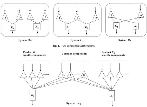
Fig. 1. Two-component ATO systems.
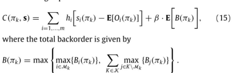
Fig. 2. ATO system withkcommon components.
Lu et al. [13] studies the NHB rules in continuous-review ATO systems of a general product structure, and identifies conditions on product and cost structure under which the NHB rules outper-form all other component allocation rules. Dogru et al. [7] studies the general class of the NHB rules in a two-product system with identical constant lead times. However, both papers do not con-sider the impact of component commonality. In addition to [15], several other papers study the value of component commonality in dynamic inventory systems with lead times [1,6,14]. They assume continuous-review inventory control and focus on the FCFS rule; although Agrawal and Cohen [1] use a fair-share rule for demand realized in the same period, the paper assumes FCFS for satisfying demand in different time periods.
In the component commonality literature, researchers have employed a representative two-product ATO system in which each product is assembled from two components [2,9] as illustrated in Fig. 1. In system
π
0, products are assembled from product-specificcomponents only and there is no common component. In system
π
1, the products share the common component 5 that replacescomponents 3 and 4 in System
π
0. In systemπ
2, the two productsshare both the common components 5 and 6 where component 6 replaces components 1 and 2 in system
π
1.In this paper, we study the value of component commonality in a generalized version of the aforementioned two-component sys-tems in Fig. 1 with lead times and the NHB rules. Using a sample path analysis, we show that under any NHB rule, both the total product backorder and total on-hand component inventory de-crease in any event as the degree of commonality inde-creases. However, the system-wide average cost does not always decrease unless a certain cost symmetric condition is imposed. Finally, we consider systems with general cost structure and conduct a numer-ical study to quantify the impact of commonality on system-wide average cost and its dependence on various system parameters.
2. The model and preliminary results
We consider a multi-product ATO system withmdifferent com-ponents labeled byi
∈ {
1,
2,
3, . . . ,
m}
. At most one unit of acomponent is required for each product. LetKdenote the set of products. Each productK
∈
Kis assembled by the component setK
⊆ {
1,
2,
3, . . . ,
m}
. For each productK∈
K, it requires a set of common componentsM(which is shared by all products) and a set of product-specific componentsK\
M. If|
M| =
k, we denote the system byπ
k. Fig. 2 provides an example with two products.In the sequel, we use subscripts to indicate components and superscripts to indicate products. Let Ki be the product set that requires componenti. We assume that the demand process
{
DK(
t),
t≥
0}
for productK∈
Kfollows an arbitrary stochastic or deterministic process which could be dependent or independent of the others, such as ARMA [8] (or a vector ARMA), ARIMA [10], quasi-ARMA [11] and MMFE [5].The component inventory is controlled by an independent continuous-time base-stock policy with base-stock levels s
=
(
s1,
s2, . . . ,
sm)
. Thanks to its simplicity, this class of inventory poli-cies is well adopted in practice and studied in the literature [16]. We note that the base-stock policy is suboptimal in a general as-sembly system, and refer the reader to [16] for a detailed review of the literature. Without loss of generality, we assume that the ini-tial on-hand inventory of componentiequalssi. For componenti, letLibe the replenishment lead time which is a constant,Ii(
t)
be the on-hand inventory at timet, andOi(
t)
be the outstanding or-der that is the amount of oror-ders placed but not replenished byt. Because the arrival of each demand requiring componentitriggers a replenishment order for this component, we haveOi
(
t)
=
X
K∈Ki
DK
(
t−
Li,
t),
(1)whereDK
(
t−
Li
,
t)
denotes lead time demand of productK dur-ing the time period(
t−
Li,
t]
. We assume full backorder for any demand which cannot be satisfied upon arrival. LetBi(
t)
be the shortage of componentiat timet, and it is expressed asBi(
t)
=
[
Oi(
t)
−
si]
+, where[
x]
+:=
max{
x,
0}
. LetBK(
t)
be the backorder of productK∈
Kat timet. For steady state variables, we omit the parametert.J. Shi, Y. Zhao / Operations Research Letters 42 (2014) 409–413 411 The following flow conservation equation holds under any
allocation rule for componenti[13].
Ii
(
t)
=
si−
Oi(
t)
+
X
K∈KiB
K
(
t).
(2)Since the on-hand inventory at any time is nonnegative, i.e.,Ii
(
t)
≥
0, by Eq. (2), we obtainX
K∈KiB K
(
t)
≥
Bi
(
t),
∀
i.
(3)An allocation rule is no-holdback (NHB) if the following condition is satisfied for allt[13,15],
BK
(
t)
×
min{
Ii(
t),
i∈
K} =
0,
for allK∈
K.
(4) In other words, under an NHB allocation rule, a product demand is backordered if and only if at least one of its required components is out of stock. For the total product backorder, Lu, et al. [13] provide the following result: for systemπ
kwith the common component setMunder an NHB allocation rule, on all sample paths, the total product backorder satisfiesX
K∈K BK(π
k,
t)
=
max(
max i∈M{
Bi(π
k,
t)
}
,
X
K∈K max j∈K\M{
Bj(π
k,
t)
}
)
.
(5) 3. Degree of commonalityWe define thedegree of commonalityto be the number of com-mon components,
|
M|
. Consider a series of ATO systems{
π
k,
k=
0
,
1,
2,
3, . . .
}
with the corresponding common component sets{
Mk,
k=
0,
1,
2,
3. . .
}
such thatM0⊂
M1⊂
M2⊂
M3⊂ · · ·
, where k= |
Mk|
. For the multi-component systemπ
k, wherek
=
0,
1,
2,
3, . . . ,
let the total product backorder at timetbeB
(π
k,
t)
=
X
K∈K
BK
(π
k,
t).
To compare the performance of systems with different degree of commonality, we investigate systems
π
kandπ
k+1. In particular,letn be the index of thecritical component such thatMk+1
=
MkS
{
n}
. Furthermore, letsn(π
k+1)
be the base-stock level of thecomponentnin system
π
k+1, andsKn(π
k)
be the base-stock level of the product-Kspecific component in systemπ
kwhich is replaced by the common componentnin systemπ
k+1. For ease ofexposi-tion, we make the following assumption.
Assumption 1. For systems
π
kandπ
k+1,(a) the lead time and holding cost for each component do not change before/after component sharing;
(b) for component n, the base-stock level is accumulated after component sharing, that is
sn
(π
k+1)
=
X
K∈K
sKn
(π
k)
;
(6)(c) for other components, the base-stock levels do not change be-fore/after component sharing.
Let On
(π
k+1,
t)
denote the outstanding order of component n in systemπ
k+1, and OKn(π
k,
t)
be the outstanding order of the product-K component in systemπ
k that is replaced by the common componentnin systemπ
k+1. Then, we have the followingobservation.
Observation 1. Under Assumption1, for the critical component n, the following result holds on all sample paths,
On
(π
k+1,
t)
=
X
K∈K
OKn
(π
k,
t).
(7)Theorem 1. For the class of general ATO systems under any base-stock levels, Assumption 1 and any NHB allocation rule, the total
product backorder decreases as the degree of commonality increases on all sample paths, that is,
B
(π
k,
t)
≥
B(π
k+1,
t),
k=
0,
1,
2,
3, . . . .
Proof. Note that for anyi
∈
Mk, by Assumption 1, we haveBi
(π
k,
t)
= [
Oi(π
k,
t)
−
si(π
k)
]
+= [
Oi(π
k+1,
t)
−
si(π
k+1)
]
+=
Bi(π
k+1,
t),
and for any product-specific componentj
∈
K\
Mk+1we haveBj
(π
k,
t)
= [
Oj(π
k,
t)
−
sj(π
k)
]
+= [
Oj(π
k+1,
t)
−
sj(π
k)
]
+=
Bj(π
k+1,
t).
By Eq. (5), we further have
B
(π
k,
t)
=
max(
max i∈Mk{
Bi(π
k,
t)
}
,
X
K∈K max j∈K\Mk{
Bj(π
k,
t)
}
)
=
max(
Q(
t),
X
K∈K max{
RK(
t),
Bn(π
k,
t)
}
)
;
(8) and B(π
k+1,
t)
=
max(
max i∈Mk +1{
Bi(π
k+1,
t)
}
,
X
K∈K max j∈K\Mk +1{
Bj(π
k+1,
t)
}
)
=
max(
max{
Q(
t),
Bn(π
k+1,
t)
}
,
X
K∈K RK(
t)
)
,
(9)where Q
(
t)
=
maxi∈Mk{
Bi(π
k,
t)
}
and RK(
t)
=
maxj∈K\Mk +1{
Bj(π
k+1,
t)
}
.
For any productK∈
K, letBKn(π
k,
t)
= [
OKn(
t)
−
sK
n
]
+. By Assumption 1, we have the following result for the total shortage of componentnbefore and after sharing,Bn
(π
k+1,
t)
= [
On(π
k+1,
t)
−
sn(π
k+1)
]
+=
"
X
K∈K(
OKn(π
k,
t)
−
sKn(π
k))
#
+≤
X
K∈K OKn(π
k,
t)
−
sKn(π
k)
+=
X
K∈K BKn(π
k,
t).
(10) Here the second equality holds by Eqs. (6) and (7), and the in-equality holds by the fact that[
P
aK
]
+≤
P
[
aK]
+ withaK=
OK
n
(π
k,
t)
−
sKn(π
k)
. To compare Eq. (8) with Eq. (9), we consider the following two cases:•
case 1:Q(
t)
≥
Bn(π
k+1,
t)
. By Eq. (9), we have B(π
k+1,
t)
=
max(
Q(
t),
X
K∈K RK(
t)
)
≤
max(
Q(
t),
X
K∈K max{
RK(
t),
BKn(π
k,
t)
}
)
=
B(π
k,
t)
;
•
case 2:Q(
t) <
Bn(π
k+1,
t)
. By Eq. (9), we have B(π
k+1,
t)
=
max(
Bn(π
k+1,
t),
X
K∈K RK(
t)
)
≤
max(
X
K∈K BKn(π
k,
t),
X
K∈K RK(
t)
)
≤
X
K∈K maxBKn(π
k,
t),
RK(
t)
=
max(
Q(
t),
X
K∈K max{
RK(
t),
BKn(π
k,
t)
}
)
=
B(π
k,
t).
Here, the first inequality holds by Eq. (10), and the second to the last by the fact that
Q
(
t) <
Bn(π
k+1,
t)
≤
X
K∈K BKn(π
k,
t)
≤
X
K∈K maxRK(
t),
BKn(π
k,
t)
.
The proof is finally concluded by cases 1 and 2 above. For system
π
k, we denote the total on-hand component inven-tory byI
(π
k,
t)
=
X
i=1,2,...
Ii
(π
k,
t).
(11)Theorem 2. Consider the class of general ATO systems under any base-stock levels, Assumption1and any NHB allocation rule. If all the products K
∈
K require the same number of components, then the total on-hand inventory decreases as the degree of commonality increases on all sample paths, that isI
(π
k,
t)
≥
I(π
k+1,
t),
k=
0,
1,
2,
3, . . .
Proof. Let
v
be the number of components required by each productK∈
K. By Eqs. (2) and (11), we rewrite the total on-hand inventory of systemπ
k, as follows,I
(π
k,
t)
=
X
i=1,2,... si(π
k)
−
X
i=1,2,... Oi(π
k,
t)
+
v
·
B(π
k,
t).
(12) Next, by Assumption 1(b), systemsπ
khave the same total base-stock level (corresponding to the first term on the right hand side of Eq. (12)). Furthermore, by Observation 1, systemsπ
khave the same total outstanding orders (corresponding to the second term on the right hand side of Eq. (12)). Finally, the proof readily followsfrom Theorem 1.
4. Average cost analysis
In this section, we consider the long-run time-average cost which is the sum of inventory holding costs of all components and backorder penalty costs of all products per unit of time. We assume a linear holding cost for each component’s on-hand inventory and a linear backorder cost for each product backorder. In particular, lethi denote the inventory holding cost per unit of componenti, andbK denote the backorder cost per unit of productK. For any base-stock policys, the expected total average cost of the system in its steady state is
C
(π
k,
s)
=
X
i=1,2,...,m hiE Ii(π
k)
+
X
K∈K bKE BK(π
k)
.
Substituting Eq. (2) into the above equation yields
C
(π
k,
s)
=
X
i=1,2,...,m hih
si(π
k)
−
E[
Oi(π
k)
]
i
+
X
K∈Kβ
KE BK(π
k)
,
(13) whereβ
K=
X
i∈Khi+
b K.
(14)System
π
kis calledcost symmetricifβ
K=
β
for each productK, where
β >
0 is a positive constant. Otherwise, it is calledcost asymmetric.Table 1
E[BK1]andE[BK2]of systemsπ0andπ1.
λK1=1 λK1=3
E[BK1] E[BK2] E[BK1] E[BK2]
Systemπ0 1.34 5.08 9.00 5.03
Systemπ1 2.00 4.07 8.40 5.61
If system
π
kis cost symmetric, then by Eqs. (13) and (5), we have the following expression:C
(π
k,
s)
=
X
i=1,...,m hih
si(π
k)
−
E[
Oi(π
k)
]
i
+
β
·
E B(π
k)
,
(15) where the total backorder is given byB
(π
k)
=
max(
max i∈Mk{
Bi(π
k)
}
,
X
K∈K max j∈K\Mk{
Bj(π
k)
}
)
.
The following theorem presents the value of component common-ality for cost-symmetric systems.
Theorem 3. Forcost-symmetric systems(i.e.,
β
K=
β
for each product K ) with any given base-stock levels,s, under Assumption1and any NHB allocation rule, the average cost decreases as the degree of commonality increases, that is
C
(π
k,
s)
≥
C(π
k+1,
s),
k=
0,
1,
2, . . .
Proof. For cost-symmetric systems
π
kandπ
k+1, we compare theaverage costs given by Eq. (15). By Assumption 1, before and after component sharing, the holding cost for each component does not change, and the base-stock level and outstanding order for each non-critical component (see Section 3 for a definition of the critical component) do not change. For the critical component, its base-stock level and outstanding order after sharing are the sums of their counterparts before sharing. Then, the first and second terms in Eq. (15) do not change after component sharing. Finally, the result readily follows from Theorem 1.
Note that Theorem 3 may not hold for a cost-asymmetric sys-tem. For example, we consider the two-component systems
π
0andπ
1illustrated in Fig. 1 under the FRFS allocation rule, and we set L1=
L2=
L6=
1 andL3=
L4=
L5=
4;
s1=
2,
s2=
2,
s3=
3
,
s4=
3,
s5=
6 ands6=
4. We assume that the demand processof each product follows an independent Poisson process with rate
λ
Ki. We setλ
K2=
2, and study the expected backorder for eachproduct while
λ
K1=
1 or 3.Table 1 exhibits the expected backorder for each product ob-tained via simulation (the simulation error is controlled within 0.5%). Because the expected backorders of individual products may not decrease as the degree of commonality increases, the average cost may not decrease for cost-asymmetric systems. For example, when
λ
K2=
1, one can choose aβ
K1that is sufficiently larger thanβ
K2such thatC(π
1
,
s) >
C(π
0,
s)
by Eq. (13). 5. Numerical studyIn this section, we conduct a numerical study to quantify the value of component commonality and its dependence on various system parameters. To this end, we consider the two-component systems
π
0andπ
1in Fig. 1 under the FRFS allocation rule. For eachinstance, we compute the minimum average cost by searching the optimal base-stock levelss∗using simulation. The percentage
sav-ing (or the value of commonality) is defined as follows, Value of commonality or % of saving
=
[
C(π
0,
s ∗)
−
C(π
1,
s∗)
]
C(π
0,
s∗)
×
100%,
whereC(π
k,
s∗)
=
minsC(π
k,
s),
k=
0,
1.J. Shi, Y. Zhao / Operations Research Letters 42 (2014) 409–413 413 Table 2
The impact of lead times on the value of commonality.
La Lb 1 2 3 4 5 6 7 8 9 10 1 7.00 18.37 18.76 20.97 20.36 22.81 27.73 35.72 46.68 57.97 2 12.79 4.87 14.81 15.97 17.71 18.21 20.46 24.12 31.33 41.73 3 11.32 13.33 7.26 14.02 16.17 16.77 18.30 18.99 22.45 29.23 4 10.14 12.06 11.63 6.06 13.57 14.32 15.81 16.65 17.74 21.11 5 9.67 12.64 12.45 11.65 5.14 12.99 15.11 15.70 16.38 17.61 6 9.39 11.88 11.94 11.87 12.54 6.46 12.36 14.58 14.94 15.67 7 9.28 11.73 11.73 11.48 12.61 11.61 6.17 11.68 13.39 14.18 8 11.07 11.99 11.56 12.35 12.76 12.71 12.95 5.09 11.49 13.36 9 15.38 13.32 11.67 11.89 12.51 12.43 14.49 17.72 5.53 11.87 10 21.93 16.90 12.95 11.85 12.30 12.25 14.17 18.52 24.39 6.20 Table 3
The impact of inventory holding cost on the value of commonality.
hb s∗(π0)=(s1,s2,s3,s4) s∗(π1)=(s1,s2,s5) C(π0,s∗) C(π1,s∗) % saving 1 (13,13,13,13) (13,13,26) 40.104 39.938 0.4149 3 (12,12,12,12) (13,13,24) 52.299 51.131 2.2328 5 (12,12,12,12) (12,13,23) 62.727 60.020 4.3153 7 (11,11,11,11) (12,12,22) 70.839 67.032 5.3742 9 (11,11,11,11) (12,12,21) 78.446 73.548 6.2432
Impact of lead time: this study tries to answer the following ques-tion: shall we share components with longer lead times or the op-posite? To this end, we set the demand arrival rates
λ
K1=
λ
K2=
1;
hi=
1 for alli; andbK1=
bK2=
20. We vary lead timesL1
=
L2=
LaandL3=
L4=
Lb, where the lead time of the common component,La, and the lead time of product-specific component,Lb, take value from 1 to 10. We calculate the value of commonal-ity for each combination ofLaandLb. The result is summarized in Table 2. We make the following observations:
•
ifLb≥
La: keepingLafixed, a longerLbtends to increase the value of commonality;keepingLbfixed, a longerLatends to de-crease the value of commonality.•
except for 5 cases, any upper diagonal element of the table is al-ways greater than its corresponding element in the lower diago-nal of the table, e.g., the value of commodiago-nality whenLa=
3 andLb
=
6 is greater than the value of commonality whenLa=
6 andLb=
3.In summary, sharing components with longer lead time tends to result in higher value of commonality. WhenLb
≥
La, the larger the difference in lead time between product-specific component and common component, the higher the value of commonality. How-ever, whenLb<
La, there is no clear trend on how lead time affects the value of commonality.Impact of component holding cost: this study tries to address the following question: shall we share expensive components or the opposite? To this end, we design a numerical study with Poisson demand arrival rates
λ
K1=
λ
K2=
1,
Li
=
10 for alli,
bK1=
bK2=
20, andh1=
h2=
3. We varyh3=
h4=
hbfrom 1, 3, 5, 7 and 9. The result is summarized in Table 3 which shows that the value of commonality always increases as the shared components become more expensive to carry in inventory. Thus, sharing more expen-sive components tends to result in higher value of commonality.Although our unconstrained model of backorders and inventory cost differs from the fill-rate constrained model of [15], our numer-ical result on the impact of lead time and inventory holding cost agrees well with those of [15]. Specifically, in both models, sharing components with longer lead times and higher inventory holding costs tends to result in a higher value of commonality.
Acknowledgments
We are grateful to Dr. Sridhar Seshadri (the Area Editor) and the reviewer for their valuable comments that have significantly improved the quality and presentation of the paper. The second author is supported in part by the career award 0747779 from the National Science Foundation.
References
[1] N. Agrawal, M. Cohen, Optimal material control and performance evaluation in an assembly environment with component commonality, Nav. Res. Logist. 48 (2001) 409–429.
[2] K.R. Baker, M.J. Magazine, H.L.W. Nuttle, The effect of commonality on safety stocks in a simple inventory model, Manag. Sci. 32 (1986) 982–988. [3] S. Benjaafar, M. ElHafsi, Production and inventory control of a single product
assemble-to-order system with multiple customer classes, Manag. Sci. 52 (2006) 1896–1912.
[4] G. Cachon, C. Terwiesch, Matching Supply with Demand, vol. 2, McGraw-Hill, New York, 2006.
[5] L. Chen, H. Lee, Information sharing and order variability control under a generalized demand model, Manag. Sci. 55 (5) (2009) 781–797.
[6] F. Cheng, M. Ettl, G.Y. Lin, D.D. Yao, Inventory-service optimization in configure-to-order system, Manuf. Serv. Oper. Manag. 4 (2002) 114–132. [7] M.K. Dogru, M.I. Reiman, Q. Wang, A stochastic programming based inventory
policy for assemble-to-order systems with application to the W model, Oper. Res. 58 (2010) 849–864.
[8] G. Gaalman, Bullwhip reduction for ARMA demand: the proportional policy versus the full-statefeedback policy, Automatica 42 (2006) 1283–1290. [9] Y. Gerchak, M.J. Magazine, A.B. Gamble, Component commonality with service
level requirements, Manag. Sci. 34 (1988) 753–760.
[10] K. Gilbert, An ARIMA supply chain model, Manag. Sci. 51 (2005) 305–310. [11] A. Giloni, C. Hurvich, S. Seshadri, Forecasting and information sharing in supply
chains under quasi-ARMA demand, IIE Trans. 46 (1) (2014) 35–54.
[12] R. Kapuscinski, R. Zhang, P. Carbonneau, R. Moore, B. Reeves, Inventory decisions in Dell’s supply chain, Interfaces 34 (2004) 191–205.
[13] Y. Lu, J.S. Song, Y. Zhao, No-holdback allocation rules for continuous-time assemble-to-order systems, Oper. Res. 58 (2010) 691–705.
[14] J.S. Song, Order-Based backorders and their implication in multi-item inventory systems, Manag. Sci. 48 (2002) 499–516.
[15] J.S. Song, Y. Zhao, The value of component commonality in a dynamic inventory system with lead times, Manuf. Serv. Oper. Manag. 11 (2009) 493–508. [16] J.S. Song, P. Zipkin, Supply Chain Operations: Assemble-to-Order Systems,
in: Handbooks in Operations Research and Management Science, vol. 11, 2003, pp. 561–596. Chapter 11.
[17] J.A. Van Mieghem, Note-commonality strategies: value drivers and equiva-lence with flexible capacity and inventory substitution, Manag. Sci. 50 (2004) 419–424.