VARIANT OF GMRES
A. H. BAKER∗, J. M. DENNIS †, AND E. R. JESSUP ‡
Abstract. The increasing gap between processor performance and memory access time warrants the re-examination of data movement in iterative linear solver algorithms. For this reason, we explore and establish the feasibility of modifying a standard iterative linear solver algorithm in a manner that reduces the movement of data through memory. In particular, we present an alternative to the restarted GMRES algorithm for solving a single right-hand side linear systemAx=bbased on solving the block linear systemAX=B. Algorithm performance, i.e. time to solution, is improved by using the matrix Ain operations on groups of vectors. Experimental results demonstrate the importance of implementation choices on data movement as well as the effectiveness of the new method on a variety of problems from different application areas.
Key words.GMRES, block GMRES, iterative methods, Krylov subspace, memory access costs
AMS subject classifications. 65F10, 65Y20
1. Introduction. We consider the solution of a large sparse system of linear equations:
Ax=b,
(1)
where A ∈ Rn×n, and x, b ∈ Rn. Iterative methods are often chosen to solve such
linear systems, and, when A is nonsymmetric, the GMRES (generalized minimum residual) [38] method is a common choice. Because linear systems are ubiquitous in science and engineering applications, improving the robustness of linear solvers continues to be of interest.
The two main costs associated with an iterative linear solver algorithm are the floating-point operations and the cost of moving data through memory, and perfor-mance may be improved by reducing either of these costs. Our focus is on achieving a balance between improving the efficiency of an iterative linear solver from a memory-usage standpoint while maintaining favorable numerical properties. In particular, the goal of this work is to demonstrate the feasibility of improving the performance of a common iterative linear solver (restarted GMRES), and likewise other itera-tive solvers, via a combination of a memory-efficient implementation and algorithmic modifications that reduce data movement.
In this paper, we report on our investigation into a memory-efficient iterative linear solver and describe the resulting new block method. We emphasize the im-plementation of the new method, numerous numerical test results, and evaluation of
∗Center for Applied Scientific Computing, Lawrence Livermore National Laboratory, Box 808 L-551, Livermore, CA 94551 ([email protected]). The work of this author was primarily supported by the Department of Energy Computational Science Graduate Fellowship Program of the Office of Scientific Computing and Office of Defense Programs in the Department of Energy under contract DE-FG02-97ER25308. Portions of this work were performed under the auspices of the U.S. Depart-ment of Energy by University of California Lawrence Livermore National Laboratory under contract No. W-7405-Eng-48.
†Scientific Computing Division, National Center for Atmospheric Research, Boulder, CO 80307-3000 ([email protected]). The work of this author was supported by the National Science Foundation. ‡Department of Computer Science, University of Colorado, Boulder, CO 80309-0430 ([email protected]). The work of this author was supported by the National Science Foun-dation under grant no. ACI-0072119.
performance based on the tracking of data movement through parts of the memory hierarchy. In Section 2 we discuss related background information. We outline our approach for improving restarted GMRES performance in Section 3. Section 4 intro-duces our new block method. We discuss implications of implementation decisions on data movement and present computational results for a variety of problems in Section 5. Finally, we give concluding remarks in Section 6.
2. Background. Though the cost of a numerical linear algebra algorithm has traditionally been measured in terms of the floating-point operations required, a more memory-centric approach has long been advocated (e.g., see [19, 16, 23]). It is well-known that matrix algorithm performance continues to be limited by the gap between microprocessor performance and memory access time (e.g., see [16, 45, 28, 26, 20, 1]). The discrepancy between DRAM (dynamic random access memory) access time and microprocessor speeds has increased by nearly 50% per year [35]. As a result, the percentage of overall application time spent waiting for data from main memory has increased [35]. The situation is compounded by advances in algorithm development that have decreased the total number of floating-point operations required by many algorithms [20]. Therefore, the number of floating-point operations required by an algorithm is not necessarily an accurate predictor of algorithm performance for a large matrix algebra problem [20]. In fact, performance bounds based on sustainable memory bandwidth (such as the STREAM [27] benchmark) are thought to predict algorithm performance most accurately [20, 1]. In particular, when solving a linear system, efficient data reuse (i.e., reducing data movement) is crucial to reducing an algorithm’s memory costs [23, 16, 19].
Krylov subspace methods such as GMRES are based on an iteration loop that accesses the coefficient matrix Aonce per loop and performs a sparse matrix-vector multiply. Thus, a desirable modification in terms of reducing data movement is to perform more than one matrix-vector product for a single memory access ofA. This optimization is natural when solving several linear systems with the same coefficient matrixAbut different right-hand sides. Such linear systems can be written as a single block linear system
AX=B,
(2)
where A ∈ Rn×n, X, B ∈ Rn×s, and the columns of B are the different right-hand
sides. By solving the block linear system (as opposed to solvings systems individu-ally),Anow operates on a group of vectors (multivector) instead of a single vector at each iteration. The matrixA is accessed from memory fewer times than it would be if each system were solved individually.
O’Leary first introduced block iterative solvers for block linear systems with sym-metric A with the Block Conjugate Gradient (BCG) and other related algorithms in [34]. For nonsymmetricA, a block version of the GMRES algorithm (BGMRES) is first described in [43], and detailed descriptions can also be found in [39, 40, 37]. BGMRES is essentially identical to GMRES, except that operations are performed with multivectors instead of single vectors. As with GMRES, the resources required by BGMRES may be impractical since storage and computational requirements increase with each iteration. In this case, a restarted version of BGMRES (BGMRES(m)) is commonly used in practice.
Several variants of the BGMRES method have been developed for both multiple and single right-hand side systems. For multiple right-hand side systems, a hybrid block GMRES method is presented in [39] that often solves the block system faster
than solving each single system individually due in part to fewer memory accesses. In addition, block methods that augment the approximation space with eigenvector approximations are given in [22, 29]. These methods are particularly useful for ma-trices that are sufficiently close to normal and have a few particular eigenvalues that inhibit convergence.
Of primary interest to us is the use of a block method on a block linear system to solve a single right-hand side system. This strategy is briefly noted as a possibility in [34] for block conjugate gradient algorithms. To our knowledge, the first mention of using Block GMRES to solve a single right-hand side system occurs in [9]. In this work, Chapman and Saad suggest that convergence may be improved for Ax = b
by using a block method with approximate eigenvectors or random vectors for the additional right-hand side vectors, particularly when convergence is hampered by a few small eigenvalues.
Also of note is a block variant of GMRES for single right-hand sides systems in [25]. This method is mathematically equivalent to standard GMRES and is imple-mented as an s-step method (matrixAperformssconsecutive matrix-vector multiplies at each iteration). The primary drawback is loss of accuracy with increasing block size (s). As with most blocked algorithms, the implementation allows for the use of level 3 BLAS (Basic Linear Algebra Subprograms) [14], and codes based on these routines often achieve good performance because they minimize data movement (e.g., see [13, 14, 20]).
3. Approach. Our approach to reducing data movement in restarted GMRES (GMRES(m)) is to modify the algorithm such that more than one matrix-vector product occurs for a single memory access of A. To this end, we investigate an alternative for solving a single right-hand side system as in (1) based on solving a corresponding block linear system as in (2). This algorithmic change requires the selection of additional starting vectors and right-hand sides.
Algorithmic changes that reduce memory access costs should not degrade the numerical properties of the original algorithm. Therefore, our goal in choosing ap-propriate families of additional right-hand sides and starting vectors was to select vectors that would accelerate convergence to the single right-hand side solution. For this reason, we looked to existing Krylov subspace method acceleration techniques.
It is well-known that subspace information is lost in GMRES(m) due to restart-ing, and a number of acceleration methods attempt to in some sense compensate for this loss (e.g., see [30, 31, 42, 12, 9, 4]). Our block method derives from the LGM-RES method [4], an augmented Krylov subspace method with appealing convergence properties. In particular, the extra right-hand sides used in the block method are the same as used to augment the standard GMRES approximation space in LGMRES.
In addition, beyond the algorithmic modifications required for a block formu-lation of GMRES(m), close attention to implementation techniques is essential for a memory-efficient, sparse linear solver. The compressed storage formats used for sparse matrices generally result in irregular patterns of memory referencing (e.g., see [18, 15]), and many approaches to improving the performance of the sparse matrix-vector multiply have been investigated (e.g., see [41, 36, 44, 19, 8, 23]). In our new block method, we reduce the cost of the additional matrix-vector operations in each iteration loop via an efficient matrix-multivector multiply routine discussed in [20, 21] that improves the performance of multiplesparse matrix-vector multiplies. This ap-proach allows the multiplication of a multivector of size four (i.e., a group of four vectors) by a matrix at about 1.5 times the cost of calculating a single matrix-vector
product. We discuss this type of matrix-multivector multiply routine and associated routines in Section 5.1.
4. A new block algorithm. In this section, we first briefly review the LGMRES method, of which the new algorithm is an extension. We then describe the new algorithm and its implementation and discuss additional considerations.
4.1. The LGMRES method. Consider GMRES(m) when solving (1). Restart parameter m denotes a fixed maximum dimension for the Krylov subspace. If con-vergence has not occurred at the end of m iterations, the algorithm restarts. We refer to the group ofm iterations between successive restarts as a cycle. We denote the restart number with a subscript: xi is the approximate solution afteri cycles or
m·itotal iterations, andri is the corresponding residual (ri =b−Axi). The min-imum residual property requires that GMRES(m) find xi+1 ∈ xi+Km(A, ri) such
that ri+1 ⊥AKm(A, ri) (e.g., see [37]), where Ki(A, ri)≡span{ri, Ari, . . . , Ai−1ri}
denotes ani-dimensional Krylov subspace.
Let ˆxbe the true solution to (1). We denote the true error after thei-th restart cycle byei, whereei≡xˆ−xi. Then the vector
zi ≡xi−xi−1
(3)
is an approximation to that error afterirestart cycles, wherezi≡0 fori <1. An error approximation is a natural choice of vector with which to augment the next approximation spaceKm(A, ri) since augmenting with the true error would solve
the problem exactly (e.g., see [17]). Furthermore, becausezi∈ Km(A, ri−1), it in some
sense represents the spaceKm(A, ri−1) generated and discarded in the previous cycle.
Therefore, the LGMRES method accelerates convergence by appendingkvectors that approximate the error from previous restart cycles to the standard Krylov approxi-mation space at the end of each restart cycle. In particular, afteri+ 1 restart cycles, LGMRES(m,k) finds an approximate solution to (1) in the following way:
xi+1=xi+qim+1−1(A)ri+ i
X
j=i−k+1 αijzj,
where polynomialqm−1
i+1 andαij are chosen such thatkri+1k2 is minimized.
4.2. The new algorithm: B-LGMRES. The augmentation scheme used by LGMRES(m, k) is easily extended to a block method by using the k previous er-ror approximations zj to build additional Krylov subspaces. We refer to this block extension as B-LGMRES(m, k), for “Block” LGMRES. Conceptually, we view one restart cycle (i) of B-LGMRES(m, k) as a cycle of Block GMRES on the system
AXi+1=B, whereB contains the right-hand side of (1) and thek most recent error
approximations zj,j= (i−k+ 1) : i. In other words,B= [b, zi, . . . , zi−k+1]. The
initial guess at restart cyclei,Xi, is then written asXi= [xi, 0, . . . , 0], where the approximate solution to our single right-hand side system, xi, is placed in the first column and the remaining columns are set to zero. X andB are sizen×(k+ 1) or
n×s, where s≡k+ 1 indicates the block size.
After i+ 1 restart cycles, the B-LGMRES(m, k) approximation space consists of the traditional Krylov portion built by repeated application of A to the current residualritogether with Krylov spaces resulting from the application ofAto previous
error approximations. Therefore, we write the B-LGMRES(m,k) approximation as
xi+1 =xi+qmi+1−1(A)ri+ i
X
j=i−k+1
αmij−1(A)zj,
(4)
where the degreem−1 polynomialsαm−1
ij andqm− 1
i+1 are chosen such thatkri+1k2is
minimized. Recall thatzi ∈ Km(A, ri−1) and thatAzi=ri−1−rifrom (3). Therefore,
by choosingzi as an additional right-hand side, the standard approximation space is augmented with part of the information generated in the previous approximation space.
Using (3), we now re-write B-LGMRES(m,k) in (4) in the following way:
zi+1=qim+1−1(A)ri+ i
X
j=i−k+1
αmij−1(A)zj.
In the above form, as shown for the LGMRES method in [4], this block method re-sembles a truncated polynomial-preconditioned full conjugate gradient method with variable preconditioning. In this analogy, the polynomial preconditioner isqmi+1−1, and
it changes at each iteration (i). In addition, the error approximation vectorszj are analogous to conjugate gradient direction vectors (e.g., see [2]), and now these direc-tion vectors are weighted by polynomials inA(αij) instead of scalars. Furthermore, as in [4], it is easily shown that these direction vectorszj areATA-orthogonal.
Theorem 1 (Orthogonality of the error approximations). The error
approxima-tion vectorszj ≡xj−xj−1 in B-LGMRES are ATA-orthogonal.
Proof. We define subspacesMi+1 andMi as
Mi+1≡ Km(A, ri) +Pji=i−k+1Km(A, zj)
Mi≡ Km(A, ri−1) + i−1 X
j=i−k
Km(A, zj).
By construction, ri ⊥AMi and ri+1⊥AMi+1.
From (3), ri−ri+1 =Azi+1⇒Azi+1⊥A(Mi∩ Mi+1).
Because{zj}j=(i−k+1):i⊂ Mi∩ Mi+1, zi+1⊥ATA{zj}j=(i−k+1):i.
To provide additional insight into the B-LGMRES augmentation scheme, we briefly describe the B-LGMRES method in the framework presented in [9]. In [9], Chapman and Saad consider the addition of an arbitrary subspace, W, to the stan-dard Krylov approximation space of a minimum-residual method, such as GMRES. This addition results in the augmented approximation space
M=K+W,
(5)
where K is the standard Krylov subspace. A minimal residual method finds an ap-proximate solution ˜x∈x0+Msuch that the residual ˜rsatisfies ˜r⊥AM, removing
components of the initial residual r0 in subspace AM via an orthogonal projection
process. Following the discussion in [9], the minimization process over the augmented approximation space (5) is
k˜rk2= min
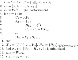
1.ri=b−Axi,β=krik2,ri=ri/β 2.Ri= [ri, zi, . . . , zi−k+1]
3.Ri=V1Rˆ (QR factorization) 4. forj= 1 :m
5. Uj=AVj 6. forl= 1 :j
7. Hl,j=VlTUj 8. Uj=Uj−VlHl,j
9. end
10. Uj=Vj+1Hj+1,j 11. end
12.Wm= [V1, V2, . . . , Vm], Hm={Hl,j}1≤l≤j+1;1≤j≤m 13. findyms.t. kβe1−Hmymk2 is minimized
14.zi+1=Wmym 15.xi+1=xi+zi+1
Fig. 1.B-LGMRES(m,k) for restart cyclei.
whered∈x0+K andw∈ W. Chapman and Saad then show that ifrd results from
minimizingkb−Adk2, where againd∈x0+K, then
k˜rk2≤ k(I−PAW)rdk2,
(6)
where PAW is an orthogonal projector onto subspace AW. In particular, for a cycle of B-LGMRES(m,k) with k= 1, we have thatK=Km(A, ri) andW=Km(A, zi) =
Km(A, ei−ei−1). Therefore, from (6) we see that the addition ofWin the B-LGMRES
method results in the removal of components of rd (the residual from the standard Krylov approximation space) from the subspace AKm(A, ei−ei−1) or, equivalently,
the removal of components of the error from subspaceKm(A, ei−ei−1).
4.3. Algorithm details. The implementation of B-LGMRES(m, k) is similar to that of BGMRES. For reference, one restart cycle (i) of B-LGMRES(m,k) is given in Figure 1. As with BGMRES, B-LGMRES(m, k) requires the application of s2
rotations at each iteration to transform Hm into an upper triangular matrix (e.g., see [37]). Because B-LGMRES(m, k) solvesAx=b, as opposed to a block system, the least squares solution step (line 13) varies from that of standard BGMRES; the triangular matrix ˆR from the QR decomposition in line 3 does not need to be saved since only β = krik2 is needed, and only s rotations must be applied to the
least-squares problem’s right-hand side (βe1) at each step.
Though we think of the error approximationszj,j= (i−k+ 1) : ias additional right-hand side vectors, we do not form the block approximate solutionsXi. Instead we append the k most recent error approximations to the initial residual to form a block residualRi, as seen in line 2 of Figure 1. We normalize the error approximations (zj/kzjk2) so that each column of the initial residual blockRi is of unit length. The msizen×sorthogonal block matricesVj form the orthogonaln×m·smatrixWm, whereWm= [V1, V2, . . . , Vm]. Hmis a size (m+ 1)s×m·sband-Hessenberg matrix
withssub-diagonals, and the following standard relationship holds:
AWm=Wm+1Hm.
As with LGMRES, onlyi error approximations are available at the beginning of restart cycles withi < k. As a result, the creation of the initial residual block in line
2 of the B-LGMRES(m, k) algorithm must be modified for the firstk cycles where
i < k. (The first cycle isi= 0.) Recall that zj ≡0 forj <1, and whenzj ≡0, we say that zj is an error approximation that is not available. In our implementation, we replace any zi, . . . , zi−k+1 that is not available with a randomly generated vector
of lengthn.
For the B-LGMRES(m, k) implementation given in Figure 1, the multivectors are of sizes, wheres=k+ 1. For example, the orthogonal block matricesVj in lines 3, 5, 8, 10, and 12 of Figure 1 are sizesmultivectors consisting ofsvectors of length
n. In addition,Riin lines 2 and 3 andUj in lines 5, 7, 8 and 10 are also multivectors. The matrix-multivector multiply occurs in line 5, and the importance of this aspect of the implementation is demonstrated in Section 5.1.
One restart cycle, or m iterations, of B-LGMRES(m, k) requires m
matrix-multivectormultiplies, irrespective of the value ofk. Therefore, matrix Ais accessed
from memory m times per cycle. For comparison, we list the approximation space size, the number of vectors of lengthnstored, and the number of matrix accesses per restart cycle in terms of parametersmandk for GMRES(m), LGMRES(m, k), and B-LGMRES(m,k) in Table 1.
Table 1
Algorithm specifications per restart cycle.
Method Approx. Lengthn Accesses
Space Size Vector Storage ofA
GMRES(m) m m+ 3 m
LGMRES(m,k) m+k m+ 3k+ 3 m
B-LGMRES(m,k) m(k+ 1) (m+ 2)k+m+ 3 m
B-LGMRES(m, k) is compatible with both left and right preconditioning. We denote the preconditioner byM−1. For left preconditioning, the initial residual in line
1 of Figure 1 must be preconditioned as usual: ri=M−1(b−Axi). Then we replaceA
withM−1Ain line 5. To incorporate right preconditioning, we replaceAwithAM−1
in line 5. We define ˆzj ≡M(xj−xj−1) =M zj and replace z with ˆz everywhere in
lines 2 and 14. While no explicit change is required for line 15 as given in Figure 1, note that, with right preconditioning, line 15 is equivalent toxi+1=xi+M−1ziˆ+1.
We note that in our implementation, no re-orthogonalization was performed, and residual norms are computed recursively at each step within a restart cycle. Addi-tionally, although deflation is often an important issue for block methods, it is not required for B-LGMRES because we are not solving a block linear system. The pos-sibility of a breakdown due to rank deficiency for the initial residual block does exist, but we have not had any breakdowns in practice (a random vector may be substituted forzi if a breakdown is detected).
5. Numerical experiments. In this section, we first give the specific details of our B-LGMRES implementation and demonstrate the advantages of some per-formance programming techniques. We then show the importance of reducing data movement to achieve an efficient implementation. Finally, we present promising ex-perimental results from our efficient implementation of B-LGMRES on a variety of problems.
We implemented the B-LGMRES algorithm in C using a locally modified version of PETSc 2.1.5 (Argonne National Laboratory’s Portable, Extensible Toolkit for Sci-entific Computation) [6, 5]. All results provided in this paper were run on a single
Table 2
List of test problems together with the matrix order (n), number of nonzeros (nnz), precondi-tioner, and a description of the application area (if known).
Problem n nnz Preconditioner Application Area
1 pesa 11738 79566 none
2 epb1 14734 95053 none heat exchanger simulation
3 memplus 17758 126150 none digital circuit simulation
4 zhao2 33861 166453 none electromagnetic systems
5 epb2 25288 175027 none heat exchanger simulation
6 ohsumi 8140 1456140 none
7 aft01 8202 125567 ILU(0) acoustic radiation, FEM
8 memplus 17758 126150 ILU(0) digital circuit simulation 9 arco5 35388 154166 ILU(0) multiphase flow: oil reservoir 10 arco3 38194 241066 ILU(1) multiphase flow: oil reservoir 11 bcircuit 68902 375558 ILUTP(.01, 5, 10) digital circuit simulation 12 garon2 13535 390607 ILUTP(.01, 1, 10) fluid flow, 2-D FEM
13 ex40 7740 458012 ILU(0) 3-D fluid flow (die swell problem) 14 epb3 84617 463625 ILU(1) heat exchanger simulation 15 e40r3000 17281 553956 ILU(2) 2-D fluid flow in a driven cavity 16 scircuit 170998 958936 ILUTP(.01, .5, 10) digital circuit simulation 17 venkat50 62424 1717792 ILU(0) 2-D fluid flow
processor of a 16-processor Sun Enterprise-6500 server with 16 Gbytes RAM. This system consists of 400 Mhz Sun Ultra II processors, each with a 16 Kbyte L1 cache and a 4 Mbyte L2 cache. For reference, Table 2 lists multiple test problems from the University of Florida Sparse Matrix Collection [11], the Matrix Market Collection [33], and the PETSc test collection.
5.1. An efficient implementation. To specifically demonstrate the benefit of an efficient implementation, we implemented B-LGMRES in PETSc 2.1.5 both with and without what we refer to as amultivector optimization. For the multivec-tor optimization implementation, theMVimplementation, we followed the previously mentioned approach in [20, 21] for improving the performance of a matrix-multivector multiply routine by grouping computations on the same data. Consider the sizes mul-tivectorV, whereV ≡[v1, v2, . . . , vs] for vectorsv1,v2,. . .,vs∈Rn×1. By processing
thesindividual vectors as a group, the matrix-multivector multiply routine performs a greater number of floating-point operations for each access of a nonzero element of the coefficient matrix A and has the potential to reduce the amount of data moved through parts of the memory subsystem by a factor of s. The approach of group-ing computations together impacts more than just the matrix multiply routine but rather pervades the implementation of the entire B-LGMRES algorithm. The second implementation, referred to as thenon-MVimplementation, does not group multivec-tor computations together and represents the best implementation possible with the tools available in PETSc. Both implementations were written so as to eliminate any copying of data from one data structure to another and represent best coding efforts. Three primary sections of the B-LGMRES code are impacted by the multivector optimization: the matrix-vector multiply (MatMult), the modified Gram-Schmidt orthogonalization (MGS), and the application of the preconditioner (Prec), if required. For the MV implementation for our set of test problems, the percentage of time spent in each of the three primary sections varies from 18% to 83% for MatMult, 6% to 55% for MGS, and 31% to 53% for Prec. Because the Prec section of code shows similar characteristics to the MatMult section, we only discuss the MatMult and
MGS sections of code. In addition, note that we concentrate on a multivector of size
s= 2 which corresponds to B-LGMRES(m, k) with k = 1. We show in Section 5.3 that sizek = 1 is generally optimal for the algorithm. However, because our results are applicable to improving the performance of general block linear solvers as well, we also discuss the advantages of a larger block size.
For the remainder of this section, we detail the MV implementation, explain how it differs from the non-MV implementation in terms of data movement, and compare the performance of the two implementations. Because algorithmic changes in a numerical code affect data movement between main memory and cache and between levels of cache, the size of the data structures determines the part of the memory most affected by the multivector optimizations. Therefore, for each we discuss theworking set size, which is the size in Mbytes of data loaded through the memory hierarchy for each operation. Note that for a typical memory hierarchy, L1 caches typically have access times of two to three clock cycles, L2 cache access times are generally 5-15 times slower, and main memory access times are generally at least 100 times slower still (e.g., see [44, 32, 7]).
The MatMult section of the code corresponds to the matrix-vector multiply in line 5 of Figure 1. For the non-MV implementation, successive calls are made to a matrix-vector multiply routine for each individual matrix-vectorv1, v2, . . . , vs in multivectorVj. In
contrast, for the MV implementation, we store the multivectors in a format referred to asmulti-component vectors in the PETSc 2.1.5 manual [5] and use the associated PETSc matrix-multivector multiply routine. This multi-component format is a row-wise storage format that storesV as a vector of lengthn·sin which the components of thesvectors are interlaced. In other words, multivector elements separated by stride
s belong to a single vector: v1 = [V(0);V(s);V(2s);. . .;V(ns−s)]. The working
set size for the MatMult section, W SM atM ult, is approximately equal to the storage required for matrixA. Therefore, for compressed sparse row storage,W SM atM ult =
sizeof(double)∗nnz+sizeof(int)∗(n+nnz), where the functionsizeof() returns the size of its argument in bytes. If W SM atM ult is significantly larger than the L2 cache size, then successive calls to a matrix-vector multiply routine repeatedly read matrixA from main memory through both levels of cache. ForW SM atM ult smaller than the L2 cache size but larger than L1, portions of matrix A may remain in L2 cache for successive matrix-vector multiplies.
The MGS section (lines 6-10 in Figure 1) often contributes significantly to the overall cost of the B-LGMRES algorithm and is dominated by the PETSc routines
VecDotandVecAXPY, which are the vector dot product and axpy routines,
respec-tively. For the MV implementation, we wrote multivector versions of these two routines, referred to as VecStrideDot and VecStrideAXPY, in a manner that lim-its movement of data. For example, in the non-MV implementation, determining the dot product of two size s multivectors, which are themselves n×s matrices, results in an s×s matrix. Computing that matrix requires s2 successive calls to
VecDot and 2·n·s2 data values to be read from the memory hierarchy. In contrast,
one call to VecStrideDot provides the same functionality, but only 2·n·s data val-ues are read because computations on related data are fused together. Therefore, if
W SM GS ≡sizeof(double)·2·n·sis greater than either the L1 or L2 cache size, the multivector optimization impacts data movement in the MGS section of code.
Both VecStrideAXPY and VecStrideDot were written using loop temporaries and loop unrolling to aid compiler optimization. The use of loop temporaries allows a compiler to identify data reuse more easily at the register level. Loop unrolling further
helps register reuse and allows different iterations of the loop to occur simultaneously. In our MV implementation we unroll the inner loop s times, where s is the block size. We chose to write our own VecStrideAXPY and VecStrideDot routines instead of using the level 3 BLAS DGEMM routine [14] due to the performance advantage of a hand-coded implementation. The timings to perform a multivector AXPY and dot product are given in Tables 3 and 4, respectively, for s = 2. The version of DGEMM labeled “src” is compiled from source code and the version labeled “opt” is the vendor supplied optimized library. Timings are given inµsec for a subset of the test problems with a range of matrix orders. For both routines, the MV and non-MV implementations are superior to DGEMM, and the hand-tuned MV implementations are the clear winners. Our MV implementations outperform DGEMM because the loops are unrolled to the specific block sizes. Because the MGS section can consume a large percentage of total execution time, the simple optimizations described can have as significant an impact on overall execution time of the solver as the use of the optimized matrix-multivector multiply routine.
Table 3
Execution times inµsecfor a single call to AXPY for the non-MV and MV implementations as well as for the standard and optimized BLAS 3 DGEMM routines with a block size ofs= 2.
Problem n non-MV MV DGEMM (src) DGEMM (opt)
13 ex40 7740 2.00 1.25 3.96 2.96
3 memplus 17758 4.55 2.85 9.18 6.73
11 bcircuit 68902 17.43 10.35 35.32 25.73
14 epb3 84617 19.54 12.58 43.49 31.88
Table 4
Execution times in µsecfor a single call to a dot product routine for the non-MV and MV implementations as well as for the standard and optimized DGEMM routines with a block size of s= 2.
Problem n non-MV MV DGEMM (src) DGEMM (opt)
13 ex40 7740 1.20 .78 3.94 2.89
3 memplus 17758 2.60 1.69 9.16 6.66
11 bcircuit 68902 10.91 6.29 35.32 24.98
14 epb3 84617 12.64 7.89 44.01 30.96
As previously explained, we store the multivectors row-wise in our MV imple-mentation. Alternatively, one might wonder whether column-wise ordering is a viable option as column-wise ordering better facilitates algorithmic needs such as deflation and requires less reorganization of data. Therefore, in Table 5, we give results for the MatMult routine on block sizes s = 2 and s = 4. MV-row and MV-col indi-cate row-wise and column-wise variations of the MV implementation. In addition to four problems from our test set, row 5 in Table 5 lists an additional problem, pois-son3Db, from the UF collection ( n= 85623 and nnz = 2374949 ) that has a large bandwidth. Our experiments indicate that the use of the column-wise storage for-mat for multivectors on large problems with a large for-matrix bandwidth causes TLB misses, as suggested in [24]. (The TLB is a cache of translations between the real and virtual addresses of recently referenced pages of memory. A TLB miss incurs two loads to memory: one to load the address translation and a second to load the actual operand.) To illustrate the impact of TLB misses, line 6 of Table 5 lists the results for the poisson3Db problem with Reverse Cuthill-McKee (RCM) [10] reordering. The
0 2 4 6 8 10 12 14 16 18 0
0.5 1 1.5 2 2.5 3 3.5
Ratio of Execution Times
non−MV / MV
Problem
MatMult MGS
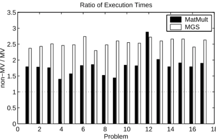
Fig. 2. A comparison of execution time for the MatMult and MGS sections with the non-MV implementation of B-LGMRES(15,1) versus the MV implementation for ten restart cycles for the 17 test problems.
RCM reordering reduces the matrix bandwidth and significantly decreases execution time for the column-wise multivector storage format. A large bandwidth does not impact the row-wise storage as much because consecutive accesses of the multivector elements correspond to data items that are stored contiguously. All further numerical experiments in this manuscript use the row-wise MV implementation.
Table 5
Execution times inµsecfor the non-MV and MV implementations of the MatMult routine for block sizess= 2ands= 4.
block size = 2 (µsec) block size = 4 (µsec)
Problem non-MV MV-row MV-col non-MV MV-row MV-col
13 ex40 30.7 24.7 25.1 47.1 27.4 27.4
3 memplus 17.8 13.4 13.4 32.4 15.7 16.2
11 bcircuit 65.3 46.2 46.5 116.4 61.9 63.1
14 epb3 84.6 57.8 60.2 134.2 71.0 75.6
- poisson3Db 424.2 263.5 369.2 831.7 367.6 927.2
- poisson3Db (RCM) 339.2 152.7 153.6 679.9 184.9 183.5
We now compare the execution times for the non-MV and MV implementations on both the MatMult and MGS sections of code in Figure 2. The x-axis corresponds to the numbered test problems in Table 2, and the y-axis is the execution time for the non-MV implementation divided by the execution time for the MV implementation. A value greater than one indicates that the execution time for MV is less than that for non-MV. For the MatMult section, the MV implementation reduces the execution time by a factor of 1.4 to 2.7 over the non-MV implementation, and it is an open question what impact matrix density (or even nonzero structure) has on the effectiveness of the multivector optimizations. For the MGS section, the execution time shows an even greater improvement on average: the MV implementation of MGS reduces execution time by a factor of 2.3 to 2.7 over the non-MV implementation. As far as the execution time for the entire B-LGMRES code, the MV implementation is close to twice as fast on average as the non-MV implementation with multivectors of size s= 2, and the performance improvement is independent of problem size (n) and number of nonzeros (nnz) for our test set in Table 2.
0 2 4 6 8 10 12 14 16 18 0
0.5 1 1.5 2 2.5 3
Ratio of MbytesL2
non−MV / MV
Problem
MatMult MGS
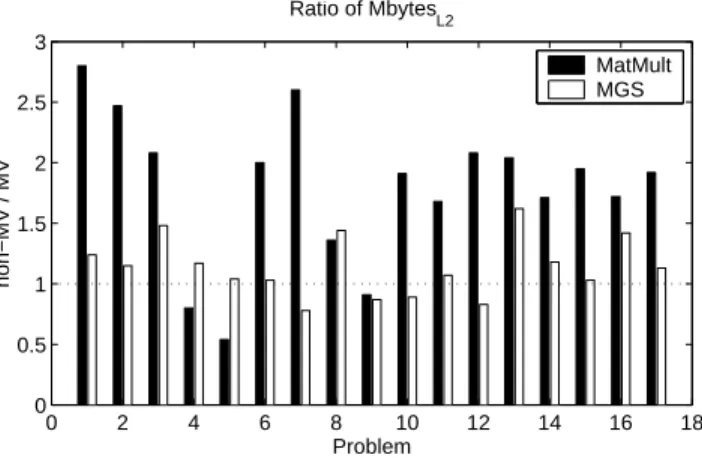
Fig. 3. A comparison of data movement from main memory to L2 cache in the MatMult and MGS sections for the non-MV implementation of B-LGMRES(15,1) versus the MV implementation for ten restart cycles for the 17 test problems.
Additionally, we remark that we modified our local installation of PETSc to include multivector versions of the PETSc routinesVecMAXPYandMatSolve. Vec-MAXPY adds a scaled sum of vectors to a vector, which is used when solving the least-squares problem. MatSolve performs a forward and back solve for use with the ILU preconditioner.
5.2. Impact of data movement on execution time. We now explain reduc-tions in execution time due to the multivector optimization using data from hardware performance counters that monitor data movement. We focus on two counters that measure the megabytes of data moved between main memory and L2 cache, denoted byM bytesL2, and between the L2 and L1 caches, denoted byM bytesL1.
We first examine data movement between main memory and the L2 cache in Figure 3. The y-axis in this figure indicates the ratio ofM bytesL2 for non-MV to MV
for both the MatMult and MGS sections. Becauses= 2, we expected a factor of two reduction inM bytesL2for the MV implementations for test problems with a working
set size significantly larger than the L2 cache. For the MatMult section, problems 6 and 11-17 haveW SM atM ultlarger than the 4 Mbytes L2 cache size. These problems all have ratios from 1.75 to 2.0, which correlate well with the factor of two reductions in execution time for those problems seen in Figure 2. For the MGS section, only problem 16 hasW SM GS greater than the L2 cache size, and this problem shows a ratio of 1.4 which does not correlate well with the factor of 2.4 improvement in execution time shown in Figure 2. Furthermore, the results in Figure 3 are inconsistent with those in Figure 2 in other ways: several problems appear to show an increase inM bytesL2
for the MGS and MatMult sections for the MV implementation. In fact, for these problems the amounts of data moved are quite small for both implementations and the apparent increases are likely the result of measurement error. Nonetheless, the MV implementation is faster than the non-MV one. These inconsistencies indicate that a reduction in M bytesL2 does not accurately predict a reduction in execution
time for MGS for most of the test problems.
We now consider data movement between the L1 and L2 caches. Figure 4 shows the ratio of M bytesL1 for the non-MV to MV implementation. For the MatMult
0 2 4 6 8 10 12 14 16 18 0
0.5 1 1.5 2 2.5 3
Ratio of MbytesL1
non−MV / MV
Problem
MatMult MGS
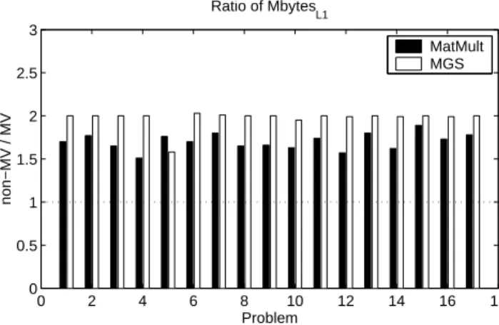
Fig. 4.A comparison of data movement from L2 cache to L1 cache in the MatMult and MGS sections for the non-MV implementation of B-LGMRES(15,1) versus the MV implementation for ten restart cycles for the 17 test problems.
reduction inM bytesL1. Test problem 1 has the smallest W SM atM ult at 978 Kbytes,
which is significantly larger than the 16 Kbyte L1 cache. Thus, Figure 4 shows that for all of the test problems the ratios of data moved do in fact range from 1.5 to 1.9. Similarly for the MGS section, problem 12 has the smallest W SM GS at 241 Kbytes, which is also significantly larger than the L1 cache. Consequently, all of the test problems have ratios that range from 1.6 to 2.0. The reduction inM bytesL1 is thus
consistent with the reduction in execution time seen in Figure 2 for both sections of code.
Therefore, from Figures 3 and 4, one can infer that the reduction intotal execu-tion time due to the MV implementaexecu-tion correlates to the reducexecu-tion inM bytesL1 for
our test problems (see [3] for more details). The importance of optimizations that reduce movement of data between levels of cache was unexpected in that emphasis is traditionally placed on reducing data movement between cache and main memory, which is of most concern to large problems. For much larger test problems, where bothW SM atM ult and W SM GS are much larger than the L2 cache size, for example, we expect that the reduction M bytesL2 would more strongly correlate to execution
time. However, our results indicate that data movement is not just an issue for very large problems. In fact, the results presented in this section demonstrate that refor-mulating an iterative solver to use multivectors enables an efficient implementation that can reduce data movement for problems of any size. Furthermore, these multivec-tor optimizations would benefit larger block sizes and other types of block methods, including those that solve systems with multiple right-hand sides.
5.3. Comparison with other methods. In this section, we demonstrate the potential of the B-LGMRES method both with and without preconditioning by pre-senting experimental results for the test problems in Table 2. If a right-hand side was not provided, we generated a random right-hand side. For all problems, the initial guess was a zero vector. For each problem we report wall clock time for the linear solve only; we do not time any I/O or the setup of the preconditioner. For the pre-conditioned problems, we use either ILU(p) or ILUTP(droptol, permtol, lf il) (e.g., see [37]). The timings reported are averages from five runs and have standard devia-tions of at most two percent. All tests are run until the relative residual norm is less
than the convergence tolerance ζ = 10−9 , i.e., when krik
2/kr0k2 ≤ ζ. However, if
a method does not converge in 1000 restart cycles, then the execution time reported reflects the time for 1000 cycles and we say that the method does not converge.
We evaluate the performance of B-LGMRES(m, k) for a particular problem by comparing its time to converge to that of GMRES(m) and LGMRES(m, k) with equal-sized approximation spaces. We use the GMRES(m) implementation available in PETSc 2.1.5 and the PETSc implementation of LGMRES(m,k) described in [4]. For GMRES(m), we chose restart parameterm= 30 because it is a common choice for GMRES(m) and is the default in PETSc. We required that the approximation spaces for both LGMRES(m,k) and B-LGMRES(m,k) be of size 30 as well. Furthermore, we wanted to evaluate the performance of LGMRES(m, k) and B-LGMRES(m, k) using the same number of error approximation vectors, i.e., the same k, for each. In choosing a value of k, we note that for LGMRES(m, k), k≤3 is typically optimal, and variations in algorithm performance are small fork≤3 (see [4]). Note that for a fixed approximation space size, increasing k for B-LGMRES(m, k) decreases the powers ofArepresented in the approximating subspace. For this set of test problems, preliminary testing showed that using k >2 was typically not beneficial, andk= 1 was generally optimal. (For an approximation space larger than 30, we expect that using k > 1 would be an advantage more often.) As a result, we chose k = 1 for the experiments presented here, and this choice together with the constraint of a size 30 approximation space determined parametermfor each method as in Table 1. Note the approximation space for B-LGMRES(15, 1) at restart cyclei+ 1 is given by K15(A, ri)+K15(A, zi) and that for LGMRES(29, 1) is given byK29(A, ri)+span{zi}.
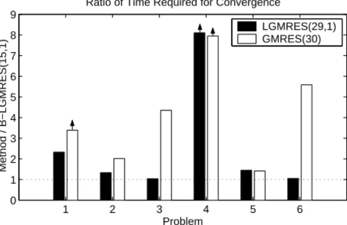
We first present results for the non-preconditioned test problems. Figure 5 com-pares the time required for convergence for B-LGMRES(15, 1) to both LGMRES(29, 1) and GMRES(30) for the test problems given in Table 2. The y-axis is the time re-quired for convergence for either LGMRES(29,1) or GMRES(30) divided by the time required for convergence for B-LGMRES(15, 1). Therefore, bars extending above one indicate faster convergence for B-LGMRES(15, 1). For all of these problems, B-LGMRES(15, 1) converges. However, arrows above the bars in Figure 5 indicate that GMRES(30) did not converge in 1000 restart cycles for problem 1 and both LGMRES(29,1) and GMRES(30) did not converge for problem 4. Again, the time for 1000 restart cycles is reported for methods that do not converge, resulting in an understated ratio of improvement for B-LGMRES(15, 1) for the bars with arrows. B-LGMRES(15, 1) converges in less time than GMRES(30) for all problems, and im-provements over LGMRES(29, 1) are more modest since LGMRES is typically also an improvement over GMRES(m) [4].
We now do the same performance evaluation for B-LGMRES(m, k) on precon-ditioned problems, problems 7-17, in Figure 6. We use left preconditioning, and determination of convergence is based on the preconditioned residual norm as usual. As in Figure 5, the bars extending above one favor B-LGMRES(15, 1). The time required for convergence for B-LGMRES(15, 1) is less than that for GMRES(30) for problems 7-15 and about the same as GMRES(30) for problems 16 and 17. However, performance gains are not as dramatic as those without preconditioning due to lower iteration counts. For large problems, though, even a small improvement in iteration count translates into a non-trivial time savings. The comparison of B-LGMRES(15, 1) to LGMRES(29, 1) is not as straightforward. The LGMRES method is quite effec-tive for these test problems, and, as a result, predicting which algorithm will “win” for a particular test problem is an open question. As an example, we tested problem
1 2 3 4 5 6 0
1 2 3 4 5 6 7 8 9
Method / B−LGMRES(15,1)
Problem
Ratio of Time Required for Convergence
LGMRES(29,1) GMRES(30)
Fig. 5.A comparison of the time required for convergence for non-preconditioned test problems 1-6 with GMRES(30) and LGMRES(29,1) versus B-LGMRES(15,1).
7 8 9 10 11 12 13 14 15 16 17 0
0.5 1 1.5 2 2.5 3
Method / B−LGMRES(15,1)
Problem
Ratio of Time Required for Convergence
LGMRES(29,1) GMRES(30)
Fig. 6.A comparison of the time required for convergence for preconditioned test problems 7-17 with GMRES(30) and LGMRES(29,1) versus B-LGMRES(15,1).
memplus both without and with preconditioning, problems 3 and 8, respectively. For this problem, B-LGMRES(15, 1) converges in slightly less time than LGMRES(29, 1) when no preconditioner is used, but LGMRES(29, 1) is faster with preconditioning.
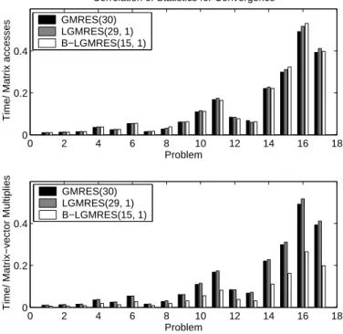
For all of the test problems in Table 2, we found that the time to solution of the restarted methods correlates well with the number of accesses of A, as opposed to the number of matrix-vector multiplies. In particular, Figure 7 illustrates that the number of accesses of A largely determines execution time. Therefore, the method that converges in the least amount of time for a particular problem in Figures 5 and 6 is generally that with the smallest number of iterations. However, it is important to acknowledge that the efficient implementation of B-LGMRES(15, 1) makes the pre-ceding statement possible because each iteration of B-LGMRES(15, 1) requires two matrix-vector multiplies; a poor implementation of B-LGMRES(15, 1) could poten-tially cost twice as much per iteration as GMRES(30).
Because our machine has sufficient resources, full GMRES is a viable option. Therefore, we also compared the time to solution of B-LGMRES(15, 1) to full GMRES for each of the 17 test problems. B-LGMRES converges in significantly less time
0 2 4 6 8 10 12 14 16 18 0
0.2 0.4
Time/ Matrix accesses
Problem
Correlation of Statistics for Convergence GMRES(30)
LGMRES(29, 1) B−LGMRES(15, 1)
0 2 4 6 8 10 12 14 16 18
0 0.2 0.4
Time/ Matrix−vector Multiplies
Problem GMRES(30)
LGMRES(29, 1) B−LGMRES(15, 1)
Fig. 7.The upper panel shows the ratios of time required for convergence to number of accesses of A for GMRES (30), LGMRES(29, 1), and B-LGMRES(15, 1) on the 17 test problems. The lower panel shows the ratios of time required for convergence to number of matrix-vector multiplies.
than GMRES on all but four problems: problems 7, 10, 13, and 15. There was no correlation between problem size and method in terms of time required for convergence for these test problems. See [3] for more details.
For the problems presented here, the time to solution of B-LGMRES(m, k) is typically an improvement over that of GMRES(m), as shown in Figures 5 and 6. The additional right-hand side vector(s) in B-LGMRES inhibit the tendency of restarted GMRES to form similar polynomials at every other restart cycle (see [4]), thus improv-ing convergence. As with the LGMRES method, B-LGMRES acts as an accelerator, but in general does not help with stalling. In other words, B-LGMRES(m,k) has a total approximation space size ofm·(k+ 1) and typically does not help problems that stall for GMRES(m·(k+ 1)), though we have found a few exceptions. For problems that stall, full GMRES or Morgan’s GMRES-DR method [31] can be good options. Although a thorough understanding of the convergence behavior of B-LGMRES is an open question that warrants further investigation, the experimental results presented in this section demonstrate that solving a single right-hand side system via a block system is a viable means of improving the time to solution of an iterative method such as GMRES(m). In particular, achieving a balance between maintaining or im-proving an iterative linear solver algorithm’s numerical properties and reducing data movement is possible.
6. Concluding remarks. In this paper, we explore the feasibility of modify-ing restarted GMRES to reduce data movement. We show that for iterative linear solvers, the time to solution is largely dependent on the number of accesses of A
modifications that reduce data movement are a particularly effective means of improv-ing performance. Furthermore, our results indicate that usimprov-ing available performance programming techniques to drive algorithm development can be effective and careful attention to implementation details can be quite beneficial. For example, hand-tuned routines can outperform subroutines such as DGEMM for certain matrix sizes, and an efficient implementation of a block version of an iterative method may be only marginally more expensive per access of coefficient matrix A than a non-block ver-sion. A unique aspect of this study is the thorough investigation of data movement through the memory hierarchy. Typically the impact of memory performance on an iterative linear solver is not studied in this detail.
Our investigation led to a block variant of the GMRES method that solves a linear system with a single right-hand side. This new method, B-LGMRES, results from choosing error approximation vectors as additional right-hand side vectors. This choice mimics a truncated polynomial-preconditioned conjugate gradient method. In our experiments, B-LGMRES performed best with a block size of two for an ap-proximation space of dimension 30. For larger apap-proximation space sizes and larger problems, a larger block size may prove more beneficial. We find that predicting the algorithm’s performance is non-trivial due to its dependence on many factors: prob-lem size (number of nonzeros and matrix order), restart parameter, block size, matrix properties, preconditioner choices, and machine characteristics. Furthermore, other right-hand side vectors may be more appropriate for particular problem classes. Given the potential performance gains from larger block sizes described in Section 5.1, our implementation of B-LGMRES can serve as a template for other block methods.
Nevertheless, the substantial improvement in performance due to reduced data movement is sufficient enticement toward pursuing block methods for single right-hand side problems. Given the increasing gap between processor performance and memory access time, re-examining popular linear solver algorithms is particularly important to achieving respectable performance on modern architectures.
REFERENCES
[1] W. K. Anderson, W. D. Gropp, D. K. Kaushik, D. E. Keyes, and B. F. Smith,Achieving high sustained performance in an unstructured mesh CFD application, in Proceedings of Supercomputing ’99, 1999. Also published as Mathematics and Computer Science Division, Argonne National Laboratory, Technical Report ANL/MCS-P776-0899.
[2] S. F. Ashby, T. A. Manteuffel, and P. F. Saylor,A taxonomy for conjugate gradient methods, SIAM Journal on Numerical Analysis, 27 (1990), pp. 1542–1568.
[3] A. H. Baker, On improving the performance of the linear solver restarted GMRES, PhD thesis, University of Colorado at Boulder, 2003.
[4] A. H. Baker, E. R. Jessup, and T. Manteuffel,A technique for accelerating the convergence of restarted GMRES, SIAM Journal on Matrix Analysis and Applications, to appear. [5] S. Balay, K. Buschelman, W. D. Gropp, D. Kaushik, M. Knepley, L. C. McInnes, B. F.
Smith, and H. Zhang,PETSc Users Manual, Tech. Report ANL-95/11 - Revision 2.1.5, Mathematics and Computer Science Division, Argonne National Laboratory, 2003. [6] S. Balay, K. Buschelman, W. D. Gropp, D. Kaushik, L. C. McInnes, and B. F. Smith,
PETSc home page. http://www.mcs.anl.gov/petsc, 2001.
[7] S. Behling, R. Bell, P. Farrell, H. Holthoff, F. O’Connell, and W. Weir, The POWER4 Processor Introduction and Tuning Guide, IBM Redbooks, November 2001. [8] S. Carr and K. Kennedy,Blocking linear algebra codes for memory hierarchies, in
Proceed-ings of the Fourth SIAM Conference on Parallel Processing for Scientific Computing, SIAM, 1989, pp. 400–405.
[9] A. Chapman and Y. Saad,Deflated and augmented Krylov subspace techniques, Numerical Linear Algebra with Applications, 4 (1997), pp. 43–66.
[10] E. H. Cuthill and J. McKee, Reducing the bandwidth of sparse symmetric matrices, in Proceedings 24th Nat. Conf. Assoc. Comp. Mach., ACM Publications, 1969, pp. 157–172. [11] T. Davis,University of Florida sparse matrix collection,
http://www.cise.ufl.edu/research/sparse/matrices, 2002.
[12] E. de Sturler,Truncation strategies for optimal Krylov subspace methods, SIAM Journal on Numerical Analysis, 36 (1999), pp. 864–889.
[13] J. W. Demmel, N. J. Higham, and R. S. Schreiber,Block LU factorization, Numerical Linear Algebra with Applications, 2 (1995), pp. 173–190.
[14] J. Dongarra, J. DuCroz, S. Hammarling, and I. Duff,A set of level 3 Basic Linear Algebra Subprograms, ACM Transactions on Mathematical Software, 16 (1990), pp. 1–17. [15] J. Dongarra and V. Eijkhout,Self-adapting numerical software for next generation
appli-cations, Tech. Report ICU-UT-02-07, LAPACK Working Note 157, August 2002. [16] J. J. Dongarra, D. C. Sorensen, and S. J. Hammarling,Block reduction of matrices to
con-densed forms for eigenvalue computations, Journal of Computational and Applied Math-ematics, 27 (1989), pp. 215–227.
[17] M. Eiermann, O. G. Ernst, and O. Schneider, Analysis of acceleration strategies for restarted minimum residual methods, Journal of Computational and Applied Mathematics, 123 (2000), pp. 261–292.
[18] B. B. Fraguela, R. Doalla, and E. L. Zapata,Cache misses prediction for high performance sparse algorithms, in Proceedings of the Fourth International Euro-Par Conference (Euro-Par ’98), 1998, pp. 224–233. Also published as University of Malaga, Department of Computer Architecture, Technical Report UNMA-DAC-98/22.
[19] K. Gallivan, W. Jalby, U. Meier, and A. H. Sameh,Impact of hierarchical memory sys-tems on linear algebra algorithm design, The International Journal of Supercomputing Applications, 2 (1988), pp. 12–48.
[20] W. D. Gropp, D. K. Kaushik, D. E. Keyes, and B. F. Smith,Toward realistic performance bounds for implicit CFD codes, in Proceedings of Parallel CFD’99, D. Keyes, A. Ecer, J. Periaux, N. Satofuka, and P. Fox, eds., Elsevier, 1999, pp. 233–240.
[21] ,High-performance parallel implicit CFD, Parallel Computing, 27 (2001), pp. 337–362. [22] G. Gu and Z. Cao,A block GMRES method augmented with eigenvectors, Applied
Mathe-matics and Computation, 121 (2001), pp. 278–289.
[23] M. S. Lam, E. E. Rothberg, and M. E. Wolf,The cache performance and optimizations of blocked algorithms, in Proceedings of the Sixth International Conference on Architectural Support for Programming Languages and Operating Systems, 1991.
[24] B. C. Lee, R. W. Vudoc, J. W. Demmel, K. A. Yelick, M. de Lorimier, and L. Zhong,
Performance optimizations for sparse matrix-multiple vector multiply, Tech. Report UCB-CSD-03-1297, Computer Science Division, University of California, Berkeley, 2003. [25] G. Li,A block variant of the GMRES method on massively parallel processors, Parallel
Com-puting, 23 (1997), pp. 1005–1019.
[26] J. D. McCalpin,Memory bandwidth and machine balance in current high performance comput-ers, IEEE Computer Society Technical Committee on Computer Architecture Newsletter, (1995). http://www.cs.virginia.edu/stream.
[27] , STREAM: Sustainable memory bandwidth in high performance computers. http://www.cs.virginia.edu/stream, 2003.
[28] S. McKee and W. Wulf, Access order and memory-conscious cache utilization, in First Symposium on High Performance Computer Architecture (HPCA1), January 1995. [29] R. Morgan,GMRES with deflated restarting and multiple right-hand sides. Presentation at
the Seventh Copper Mountain Conference on Iterative Methods, March 2002.
[30] R. B. Morgan,A restarted GMRES method augmented with eigenvectors, SIAM Journal on Matrix Analysis and Applications, 16 (1995), pp. 1154–1171.
[31] R. B. Morgan,GMRES with deflated restarting, SIAM Journal on Scientific Computing, 24 (2002), pp. 20–37.
[32] S. Naffziger and G. Hammond,The implementation of the next generation 64b Itanium microprocessor, in Proceedings of the IEEE International Solid-State Circuits Conference, vol. 2, 2002, pp. 276–504.
[33] National Institute of Standards and Technology, Mathematical and Computational Sciences Division,Matrix Market. http://math.nist.gov/MatrixMarket, 2002.
[34] D. O’Leary,The block conjugate gradient algorithm and related methods, Linear Algebra and its Applications, 29 (1980), pp. 293–322.
[35] D. Patterson, T. Anderson, N. Cardwell, R. Fromm, K. Keeton, C. Kozyrakis, R. Thomas, and K. Yellick,A case for intelligent RAM, IEEE Micro, (1997), pp. 34–44. [36] A. Pinar and M. T. Heath,Improving performance of sparse matrix-vector multiplication, in
Proceedings of Supercomputing ’99, November 1999.
[37] Y. Saad,Iterative Methods for Sparse Linear Systems, PWS Publishing Company, 1996. [38] Y. Saad and M. Schultz, GMRES: A generalized minimal residual algorithm for solving
nonsymmetric linear systems, SIAM Journal on Scientific and Statistical Computing, 7 (1986), pp. 856–869.
[39] V. Simoncini and E. Gallopoulos,An iterative method for nonsymmetric systems with mul-tiple right-hand sides, SIAM Journal on Scientific Computing, 16 (1995), pp. 917–933. [40] ,Convergence properties of block GMRES and matrix polynomials, Linear Algebra and
its Applications, 247 (1996), pp. 97–119.
[41] S. Toledo,Improving the memory-system performance of sparse-matrix vector multiplication, IBM Journal of Research and Development, 41 (1997), pp. 711–725.
[42] H. A. van der Vorst and C. Vuik,GMRESR: a family of nested GMRES methods, Numerical Linear Algebra with Applications, 1 (1994), pp. 369–386.
[43] B. Vital,Etude de quelques m´ethodes de r´esolution de probl`emes lin´eaires de grande taille sur multi-processeur, PhD thesis, Universit´e de Rennes I, Rennes, 1990.
[44] R. Vudoc, J. Demmel, K. A. Yelick, S. Kamil, R. Nishtala, and B. Lee,Performance opti-mizations and bounds for sparse matrix-vector multiply, in Proceedings of Supercomputing ’02, 2002.
[45] W. A. Wulf and S. A. McKee,Hitting the wall: Implications of the obvious, Tech. Report CS-94-48, University of Virginia, Department of Computer Science, 1994.