Visualization, Clustering and Classification of
Multidimensional Astronomical Data
Antonino Staiano
∗, Angelo Ciaramella
∗, Lara De Vinco
‡, Ciro Donalek
†, Giuseppe Longo
†, Giancarlo Raiconi
∗,
Roberto Tagliaferri
∗, Roberto Amato
†, Carmine Del Mondo
†, Giuseppe Mangano
†, Gennaro Miele
†∗Dipartimento di Matematica ed Informatica, Universit`a di Salerno, Fisciano (Sa), Italy Email:{astaiano, rtagliaferri, ciaram, gianni}@unisa.it
†Dipartimento di Scienze Fisiche, Universit`a Federico II di Napoli, Italy Email:{longo, donalek}@na.infn.it
‡INFOTEL S.r.l., Via Strauss, 45 - 84091 Battipaglia (Sa), Italy Email: [email protected]
Abstract— Due to the recent technological advances, Data
Mining in massive data sets has evolved as a crucial research field for many if not all areas of research: from astronomy to high energy physics, to genetics etc. In this paper we discuss an implementation of the Probabilistic Principal Surfaces (PPS) which was developed within the framework of the AstroNeural collaboration. PPS are a nonlinear latent variable model which may be regarded as a complete mathematical framework to accomplish some fundamental data mining activities such as: visualization, clustering and classification of high dimensional data. The effectiveness of the proposed model is exemplified referring to a complex astronomical data set.
I. INTRODUCTION
The explosive growth in the quantity, quality and accessi-bility of data which is currently experienced in all fields of science and human endeavor, has triggered the search for a new generation of computational theories and tools capable to assist humans in extracting useful information (knowledge) from the available and planned massive data sets. This revolu-tion has two main aspects: on the one hand in astronomy (as well as in high energy physics, genetics, social sciences, and in many other fields) traditional interactive data analysis and data visualization methods have proved to be far inadequate to cope with data sets which are characterized by huge volumes and/or complexity (ten or hundreds of parameter or features per record, cf. [1] and references therein). In second place, the simultaneous analysis of hundreds of parameters unveils previously unknown patterns which may lead to a deeper understanding of the underlaying phenomena and trends.
The field of Data Mining is therefore becoming of paramount importance not only in its traditional arena but also as an auxiliary tool for almost all fields of research. In this paper we discuss how three common tasks in data analysis (data visualization, clustering and data classification) may be performed using Spherical Probabilistic Principal Surfaces (PPS) as a common framework.
• Visualization: it is a crucial step in the process of data analysis, enabling an understanding of the relations that exists within the data by displaying them in such a way that the discovered patterns are emphasized.
• Clustering: it is perhaps the most important and widely used method of unsupervised learning. It may be syn-thetised problem of identifying groupings of similar points that are relatively ’isolated’ from each other, or in other words to partition the data into dissimilar groups of similar items.
• Classification: it concerns with assigning a given pattern to one of a number of possible classes which depends on the problem at hand. Such classes may be the results of a labeling accomplished on groupings resulting from a clustering procedure.
PPS [6], [7] (discussed in Section II) are a nonlinear exten-sion of principal components, in that each node on the PPS is the average of all data points that projects near/onto it. From a theoretical standpoint, the PPS is a generalization of the Generative Topographic Mapping (GTM) [2], [3], which can be seen as a parametric alternative to Self Organizing Maps (SOM) [10]. Some advantages of PPS includes its parametric and flexible formulation for any geometry/topology in any dimension, guaranteed convergence (indeed the PPS training is accomplished through the Expectation-Maximization algo-rithm). A PPS is governed by its latent topology and, owing to their flexibility, a variety of PPS topology can be created one of which is the 3D sphere. The sphere is finite and unbounded, with all nodes distributed at the edge, it therefore is ideal for emulating the sparseness and peripheral property of high-D data. Furthermore, the sphere topology can be easily comprehended by humans and thereby be og great help in visualizing high-D data (Section III-A). Since PPS generates a probability density function of the input data, in the form of a mixture of Gaussians, it can be used both for clustering (Section III-B) and classification (Section III-C) purposes. To illustrate the power and the effectivness of the model, we shall discuss a case study in the field of astronomy using a real and complex data set (Section IV). All results discussed here were obtained in the framework of the AstroNeural collaboration: a joint project between the Department of Mathematics and Informatics of the University of Salerno and the Department of Physical Sciences of the University Federico II in Napoli.
The main goal of the collaboration is to implement a user friendly data mining tool capable to deal with heterogeneous, high dimensionality data sets.
II. PPS:THEORETICAL DESCRIPTION
PPS defines a non-linear, parametric mapping y(x;W) from a Q-dimensional latent space (x ∈ RQ) to a D -dimensional data space (t ∈ RD), where normally Q < D. The mappingy(x;W)(defined continuous and differentiable) maps every point in the latent space to a point into the data space. Since the latent space is Q-dimensional, these points will be confined to a Q-dimensional manifold non-linearly embedded into the D-dimensional data space. PPS builds a constrained mixture of Gaussians (where the priors are all fixed to M1) p(t|W,Σm) = 1 M M X m=1 p(t|xm,W,Σm), (1)
and each component has the form:
|Σm|− 1 2 2πD2 e{−1 2(y(xm;W)−t)Σm−1(y(xm;W)−t)T}, (2)
wheretis a point in the data space andΣ−1
m denotes the noise
variance.
The covariance is defined as Σm=α β Q X q=1 eq(x)eTq(x) + (D−αQ) β(D−Q) D X d=Q+1 ed(x)eTd(x), (3) 0< α < D Q
whereαis a clamping factor which determines the orientation of the covariance, and
• {eq(x)}Qq=1 is the set of orthonormal vectors tangential
to the manifold at y(x;w),
• {ed(x)}Dd=Q+1 is the set of orthonormal vectors orthog-onal to the manifold in y(x;w).
The complete set of orthonormal vectors {ed(x)}Dd=1 spans
RD. The EM algorithm[8] can be used to estimate the PPS
parametersW andβ, while the clamping factor is fixed by the user and is assumed to be constant during the EM iterations. The form of the mapping y(x;w)is defined as a generalized linear regression model
y(x;w) =Wφ(x) (4) where the elements ofφ(x)consist ofLfixed basis functions
{φl(x)}lL=1, andWis aD×L matrix. A. Spherical PPS
If Q = 3 is chosen, a spherical manifold [6] can be con-structed using a PPS with nodes{xm}Mm=1 arranged regularly
on the surface of a sphere in R3 latent space, with the latent
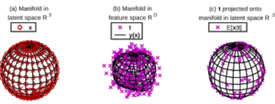
basis functions evenly distributed on the sphere at a lower density. (a) Manifold in latent space R3 x (b) Manifold in feature space RD t y(x) (c) t projected onto manifold in latent space R3
E[x|t]
(
(
Fig. 1. (a) The spherical manifold inR3 latent space. (b) The spherical
manifold inR3 data space. (c) Projection of data points tonto the latent
spherical manifold.
III. APPLICATION OFPPSTODATAMINING
A. Visualization
After a PPS model is fitted to the data, several visualization possibilities are available for analyzing the data points.
1) Data point projections onto the latent sphere: The data
are projected into the latent space as points onto a sphere (Figure 1).
The latent manifold coordinates ˆxn of each data point tn
are computed as ˆ xn≡ hx|tni= Z xp(x|t)dx= M X m=1 rmnxm
wherermn are the latent variable responsibilities defined as
rmn=p(xm|tn) = PMp(tn|xm)P(xm) m0=1p(tn|xm0)P(xm0) =PMp(tn|xm) m0=1p(tn|xm0) . (5) Since kxmk= 1 and P mrmn = 1, forn= 1, . . . , N, these
coordinates lie within a unit sphere, i.e. kˆxnk ≤1.
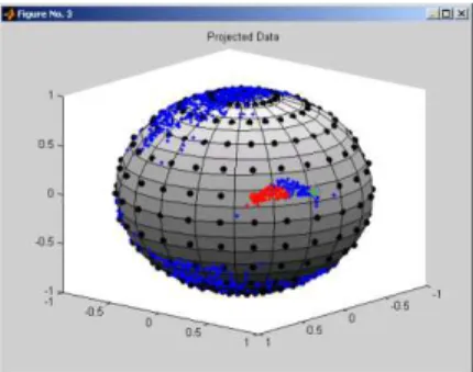
2) Interactively selecting points on the sphere: Having
projected the data on the latent sphere, a typical task per-formed by most data analyzers is the localization of the most interesting data points, for instance the ones lying far away from more dense areas (outlayers), or those lying in the overlapping regions between clusters, and to investigate their characteristics by linking the data points on the sphere with their position in the original data set. For instance, in the astronomical application described in Section IV if the images corresponding to the data were available, the user might want to visualize the object corresponding to the data point selected on the sphere. The user is also allowed to select a latent variable and color all the points for which that specific latent variable is responsible (Figure 2).
3) Visualizing the latent variable responsibilities on the sphere: Some insights on the number of agglomerates
local-ized into the spherical latent manifold is provided by the mean of the responsibility for each latent variable. Furthermore, if we build a spherical manifold which is composed by a set of faces each one delimited by four vertices, then we can color each face with colors varying in intensity on the basis of the value of the responsibility associate to that given vertex (and hence, to each latent variable). The overall result is that the sphere will contain regions denser than others and this information is easily visible and understandable (see Figure 3). Obviously, denser areas of the spherical manifold
Fig. 2. Data points selection phase. The bold black circles represent the latent variables; the blue points represent the projected input data points. When a latent variable is selected, each projected point for which the variable is responsible is colored. By selecting a data point the user is provided with information about it: coordinates and index corresponding to the position in the original catalog.
might contain more than one cluster, and this calls for further investigations.
Fig. 3. Probability density function on the latent sphere
B. Clustering
Once the user has an overall idea of the number of clusters on the sphere, he can exploit this information through the use of agglomerative hierarchical clustering techniques [9] to find out the clusters. This task is accomplished by running the clustering algorithm on the Gaussian centers in the data space. Once the center have been agglomerated, the points for which the centers falling in the same agglomerate are responsible, are assigned to the same cluster. The projections of the points into the latent space are then used to visualize the clusters onto the latent sphere [11] (see Fig. 4).
C. Classification
Classification can be accomplished in a twofold way: i) by constructing a reference manifold for each class
defined in the classification problem, and then assigning any test point to the class of its nearest manifold (PPSRM);
ii) assigning a test data choosing the class with the max-imum posterior class probability for a given new in-put(PPSPR).
Fig. 4. Clusters computed in data space by hierarchical clustering.
In [11] it was shown that this second form of classification leads to better performance. However, since PPS builds a prob-ability density function as a mixture of Gaussian distributions trained through EM algorithm, its performance may degrade with increasing data dimensionality due to singularities and local maxima in the log-likelihood function, therefore we propose two schemes for designing a committee of spheri-cal PPS to gain improved probability density functions and hence classification rates. The area of ensembles of learning machines is now a well defined field and has been successfully applied to neural networks especially in the case of supervised learning algorithms. Fewer cases can be found to unsupervised learning methodologies and to density estimation as well: among these, the works introduced in [13] and [14] both exploits consolidated techniques in supervised contexts as stacking [15] and bagging [5] and represent the basis of our implementations.
1) Stacked PPS: StPPS: The combining scheme herein
described may be seen as an instantiation of the method proposed in [14]. Let us suppose we are given withS prob-abilistic principal surface models (i.e., S density estimators)
{P P Ss(t)}Ss=1, whereP P Ss(t)is thes-th PPS model. Note
that in the original formulation given in [14], the S density estimators could also be of different kind, for example finite mixtures with a fixed number of component densities or kernel density estimate with a fixed kernel and a single fixed global bandwidth in each dimension.
Each of the S PPS models can be chosen to be diverse enough, i.e. by considering different number of latent variables and latent bases. To stack the S PPS models, we follow the procedure described below:
i) LetDthe training data set, with size|D|=N. Partition D v times, as in v-fold cross-validation. The v-th fold contains exactly(v−1)N
v training data points andNvtest
data points both from the training setD. For each fold: a) fit each of theSPPS models to the training subset
of D.
b) evaluate the likelihood of each data point in the test partition of D, for each of theSfitted models. ii) At the end of these preliminary steps, we obtain S
are organized in a matrixA, of sizeN×S, where each entryaisis P P Ss(ti);
iii) Use the matrix A to estimate the combination coeffi-cients{πs}Ss=1 that maximize the log-likelihood at the
pointsti of a stacked density model of the form: StPPS(t) =
S
X
s=1
πsP P Ss(ti)
which corresponds to maximize
N X i=1 ln à S X s=1 πsP P Ss(t) ! ,
as a function of the weight vector(π1, . . . , πS). Direct
maximization of this function is a non-linear optimiza-tion problem. We can apply the EM algorithm directly, by observing that the stacked mixture is a finite mixture density with weights (π1, . . . , πS). Thus, we can use
the standard EM algorithm for mixtures, except that the parameters of the component densitiesP P Ss(t)are
fixed and the only parameters allowed to vary are the mixture weights.
iv) The concluding phase consists in the parameters re-estimation of each of the S component PPS models using all of the training data D. The stacked density model is then the linear combination of the so obtained component PPS models, with combining coefficients
{πs}Ss=1.
2) Bagged PPS: BgPPS: This combining scheme
employ-ees bagging as mean to average a single PPS in a way similar to the model proposed in [13]. All we have to do is to train a number S of PPS with S bootstrap replicates of the original learning data set. At the end of this training process, we obtain
S different density estimates which are then averaged to form the overall density estimate model. Formally speaking, let D be the original training set of size N and {P P Ss}Ss=1 a set
of PPS models:
i) create S bootstrap replicates (with replacement) of D,
{DBoot(s)}Ss=1 with sizeN;
ii) train each of theSPPS models with a bootstrap replicate
DBoot;
iii) at the end of the training we obtainS density estimates
{P P Ss}Ss=1;
iv) average theS density estimates{P P Ss}Ss=1 as BgPPS(t) = 1 S S X s=1 P P Ss(t).
IV. CASESTUDY
The GOODS (id est the Great Observatories Origin Deep
Surveys) catalog is a catalog composed by28405objects (both galaxies and stars). The survey was conducted in 7 optical bands, namely U,B,V,R,I,J,K bands and for for the experiments described here we considered3different parameters (i.e., Kron radius, Flux and Magnitudes) for each band, thus summing to a total number of 21 parameters. The experiment’s catalog
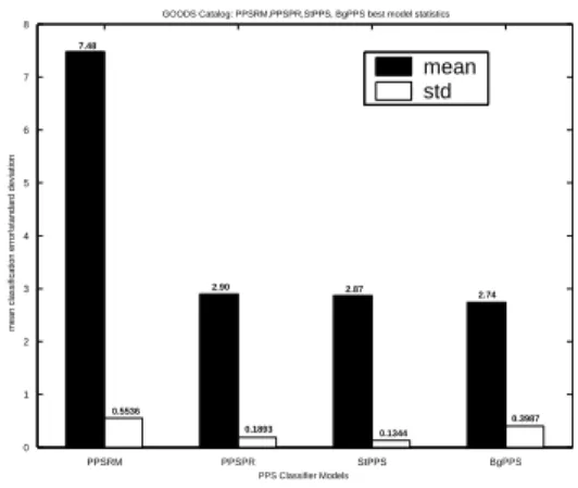
PPSRM PPSPR StPPS BgPPS 0 1 2 3 4 5 6 7 8 PPS Classifier Models
mean classification error\standard deviation
GOODS Catalog: PPSRM,PPSPR,StPPS, BgPPS best model statistics
mean std 7.48 0.5536 0.1893 0.1344 0.3987 2.90 2.87 2.74
Fig. 7. GOODS Catalog: PPSRM, PPSPR, StPPS and BgPPS best model
statistics
therefore contains about27000galaxies and 1400stars. From a computational point of view, the main peculiarity of this data set is that the majority of the objects are ”drop outs”, i.e. they are not detected in at least one of the bands (id est, not detected in only one band, two bands, three bands and so on). The data set, therefore, contains four classes of objects, namely star (S), galaxy (G), star which are drop outs (SD) and galaxy which are drop outs (GD) (we do not care about the number of bands for which an object is a drop out).
A. GOODS Catalog Visualizations
As it can be seen from Figure 5(a), the PCA visualization of the GOODS catalogue provides no interesting information at all and displays only a single condensed group of data. In PCA, the class of galaxies which are drop outs (whose objects are yellow colored), which contains the majority of objects (about
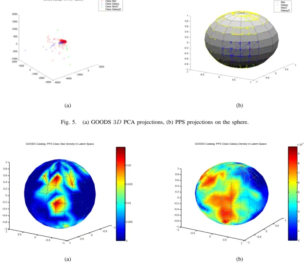
24000) is near totally hidden. The PPS projections (Figure 5(b)), instead, show a large group consisting of the drop out galaxies and overlapping objects of the remaining objects and a well bounded group of galaxies. Figure 6(a) and 6(b) also depict the latent variable probability densities for galaxy and star objects, respectively. Note, especially, how different these densities appear for each group of objects.
B. GOODS Catalog Classification
GOODS catalog classification task is very complex. As it had to be expected on the grounds of astronomical expertise, the four classes are heavily overlapping and even in the best cases there are classes (i.e., S and SD) whose objects are classified with an error rate about60%.
This is evident from the results obtained by the different PPS classifiers we compared, namely PPSRM, PPSPR, StPPS and BgPPS. Anyway, ensembles of PPS perform better than single PPS as it can be seen in Figure 7. BgPPS, in particular, obtain the best performance with a best case classification error of 2.15% as shown in Table I. The BgPPS parameter setting is shown in Table II.
(a) (b)
Fig. 5. (a) GOODS3DPCA projections, (b) PPS projections on the sphere.
−1 −0.5 0 0.5 1 −1 −0.5 0 0.5 1 −1 −0.8 −0.6 −0.4 −0.2 0 0.2 0.4 0.6 0.8 1
GOODS Catalog: PPS Class Star Density in Latent Space
0 0.005 0.01 0.015 0.02 (a) −1 −0.5 0 0.5 1 −1 −0.5 0 0.5 1 −1 −0.8 −0.6 −0.4 −0.2 0 0.2 0.4 0.6 0.8 1
GOODS Catalog: PPS Class Galaxy Density in Latent Space
0 1 2 3 4 5 6 7 8 9 x 10⁻³ (b)
Fig. 6. (a) galaxy density on the sphere (b) star density on the sphere.
TABLE I
GOODS CATALOG:CONFUSION MATRIX COMPUTED BYBgPPSBEST MODEL
Classifier Confusion Matrix α
BgP P S(2.15) S G SD GD S 155 35 12 5 G 8 1160 6 8 SD 0 0 64 7 GD 5 51 108 9740 1.8
V. CONCLUSIONS AND FUTURE WORK
We have described how spherical PPS works as a frame-work to address data mining activities such as visualization, clustering and classification and we have seen its power and effectiveness when dealing with high-Ddata as the astronom-ical data. Above all, the spherastronom-ical PPS, which consists of a spherical latent manifold lying in a three dimensional latent space, is better suitable to high-D data since the sphere is
TABLE II
GOODS CATALOG: BgPPSPARAMETER SETTINGS
Parameter Value Description
M 266 number of latent variables
L 83 number of basis functions
Lf ac 1 basis functions width iter 100 maximum number of iteration
² 0.01 early stopping threshold
able to capture the sparsity and periphery of data in large input spaces which are due to the curse of dimensionality. Currently we are pursuing two directions to further enhance our system: i) developing a clustering algorithm able to directly ex-ploit the PPS mixture Gaussian density to compute the clusters. The algorithm is based on the Kullback-Leibler distance to decide if two Gaussian component of the PPS mixture model must be aggregated. In this way the clustering is able to follow the input data density and to
compute by itself the number of clusters.
ii) building a hierarchical PPS for constructing localized nonlinear projection manifold as already done for GTM [12] and previously for a linear latent variable model [4]. Following [12], a hierarchy of PPS could be organized in a tree whose root corresponds to the PPS model trained on the entire data set at hand, and whose nodes, built interactively in a top-down fashion, represent PPS mod-els trained in localized regions of the data input chosen in the ancestor plot PPS by the user, interactively. In all the sub-models one might exploit all the visualization and clustering options discussed in this paper.
ACKNOWLEDGMENT
The authors would like to thank all past and present mem-bers of the Astroneural collaboration. Astroneural is sponsored by the MIUR (Italian Bureau for University and Research) and by Regione Campania. The authors also wish to thank P. benvenuti for many discussions and for supporting this work since its beginning.
REFERENCES
[1] J. Abello, P.M. Pardalos, M.G.C. Resende Editors: Handbook of Massive Data Sets, Kluwer Academic Publishers (2002)
[2] C. M. Bishop, M. Svensen, C.K.I. Williams, “GTM: The Generative Topographic Mapping,” Neural Computation, 10(1), 1998.
[3] C.M. Bishop, M. Svens´en, and C. K. I. Williams, “Developments of the Generative Topographic Mapping,” Neurocomputing 21, 1998. [4] C.M. Bishop and M.E. Tipping, A hierarchical latent variable model for
data visualization, IEEE Transactions on Pattern Analysis and Machine
Intelligence 20(3), 281293,1998
[5] L. Breiman, “Bagging Predictors,” Machine Learning, 26, 1996 [6] K. Chang, “Nonlinear Dimensionality Reduction Using Probabilistic
Principal Surfaces,” PhD Thesis, Department of Electrical and Computer Engineering, The University of Texas at Austin, USA, 2000
[7] K. Chang, J. Ghosh, “A unified Model for Probabilistic Principal Sur-faces,” IEEE Transaction on Pattern Analysis and Machine Intelligence, Vol. 23, NO. 1, 2001
[8] A.P. Dempster, N.M. Laird, D.B. Rubin, Maximum-Likelihood from
Incomplete Data Via the EM Algorithm, J. Royal Statistical Soc., Vol.
39, NO. 1, 1977
[9] R.O. Duda, P.E. Hart, D.G. Stork, Pattern Classification, John Wiley and Sons, 2001
[10] T. Kohonen, Self-Organizing Maps, Springer-Verlag, Berlin, (1995) [11] A. Staiano, “Unsupervised Neural Networks For The Extraction of
Scientific Information from Astronomical Data,”PhD Thesis, University of Salerno, Italy, 2003
[12] P. Tino, I. Nabney,Hierarchical GTM: constructing localized non-linear
projection manifolds in a principled way, IEEE Transactions on Pattern
Analysis and Machine Intelligence, in print
[13] D. Ormoneit, V. Tresp, “Averaging, Maximum Likelihood and Bayesian Estimation for Improving Gaussian Mixture Probability Density Esti-mates,” IEEE Transaction on Neural Networks, Vol.9, NO. 4, 1998 [14] P. Smyth, D.H. Wolpert, “An evaluation of linearly combining density
estimators via stacking,”Machine Learning, Vol. 36, 1999.