Contents
Preamble 3
Credits . . . 3
License . . . 5
1 Basic Simulation Environment 9 1.1 Introduction . . . 9
1.2 General Use . . . 9
1.2.1 Problem Description . . . 9
1.2.2 Product Delineation and Employment Domains . . . 10
1.2.3 Processed Data Types and Capabilities . . . 11
1.3 System Overview . . . 11
1.4 Components . . . 13
1.4.1 Mathematical – Physical – Modules . . . 14
1.4.2 Computational Grid . . . 14
1.5 Simulation Procedure . . . 19
1.5.1 Flow of main activities . . . 19
1.5.2 Scenario Examples . . . 21
2 Simulation procedure 25 2.1 Run BASEMENT with graphical user interface (GUI) . . . 25
2.2 Run BASEMENT on Microsoft Windows . . . 25
2.3 Run BASEMENT on Linux . . . 25
2.4 Run BASEMENT in batch mode . . . 26
2.5 Restart the simulation in BASEplane from a given solution . . . 27
3 Preprocessing 29 3.1 General . . . 29 3.1.1 Requirement . . . 29 3.1.2 Project / Scenarios . . . 29 3.1.3 Input data . . . 29 3.1.4 Boundary conditions . . . 30
3.1.5 Source terms and local properties . . . 30
3.2 Model input data . . . 31
3.2.1 Topographic data sources . . . 31
3.2.2 River related data sources . . . 34
3.2.3 Characteristic quantities of riverbed . . . 35
3.2.4 Processing the raw data . . . 37 1
Contents BASEMENT System Manuals
3.2.5 GIS Interface . . . 38
3.3 Grid generation . . . 39
3.3.1 Introduction . . . 39
3.3.2 Topographical input data . . . 40
3.3.3 Mesh quality . . . 40
3.3.4 Issues on triangulation . . . 42
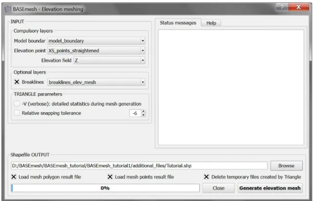
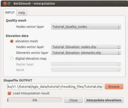
3.3.5 Use of QGIS plugin BASEmesh for grid generation . . . 46
4 Model Setup 61 4.1 General . . . 61
4.2 The Graphical User Interface (GUI) . . . 62
4.2.1 The BASEMENT Main Window . . . 62
4.2.2 General Topics of Editing Files . . . 63
4.3 Edit Command File . . . 65
4.3.1 The “BASEMENT Command File Editor” . . . 65
4.3.2 Create New or Edit Existing Command File . . . 67
4.3.3 Tools . . . 67
4.4 Edit 1-D Grid . . . 69
4.4.1 The “BASEMENT 1-D Grid File Editor” . . . 69
4.4.2 Create New or Edit Existing Geometry File . . . 69
4.4.3 Tools . . . 70
4.5 Built-In GUI Tools . . . 79
4.5.1 Interactive Visualization during run time using BASEviz . . . 79
4.5.2 Manual Controller Interface (HID) . . . 80
5 Advanced features 83 5.1 Parallelization . . . 83
5.1.1 Overview . . . 83
5.1.2 Parallelization issues on shared memory systems . . . 84
5.1.3 Parallelization with OpenMP . . . 87
5.2 Model Coupling . . . 90
5.2.1 Introduction . . . 90
5.2.2 Coupling Types . . . 90
5.2.3 Coupling Mechanisms . . . 93
5.2.4 Definitions of Exchange Conditions . . . 94
5.2.5 Synchronization Concept . . . 98
5.2.6 External Coupling . . . 101
5.3 Flow Control in River Systems . . . 103
5.3.1 Introduction . . . 103
5.3.2 Concept of Flow Control . . . 104
5.3.3 Controller Types . . . 105
Preamble
VERSION 2.8.1 November, 2020
Credits
Project TeamSoftware Development, Documentation and Test (alphabetical) M. Bürgler, MSc. ETH Environmental Eng.
F. Caponi, MSc. Environmental Eng. Dr. D. Conde, MSc. Civil Eng. E. Gerke, MSc. ETH Civil Eng.
S. Kammerer, MSc. ETH Environmental Eng. Dr.techn. M. Weberndorfer, MSc.
Scientific Board
Prof. Dr. R. Boes, Director VAW, Member of Project Board Dr. A. Siviglia, MSc, Scientific Adivisor
Dr. D. Vanzo, MSc. Environmental Eng., Scientific Adivisor Dr. D. Vetsch, Dipl. Ing. ETH, Project Director
Former Project Members
Seehttps://www.basement.ethz.ch/people
Contents BASEMENT System Manuals Cover Page Art Design
W. Thürig
Commissioned and co-financed by
Swiss Federal Office for the Environment (FOEN)
Contact
website: http://www.basement.ethz.ch
user forum: http://people.ee.ethz.ch/~basement/forum
© 2006–2020 ETH Zurich / Laboratory of Hydraulics, Glaciology and Hydrology (VAW) For list of contributors see www.basement.ethz.ch
Citation Advice For System Manuals:
Vetsch D., Siviglia A., Bürgler M., Caponi F., Ehrbar D., Facchini M., Faeh R., Farshi D., Gerber M., Gerke E., Kammerer S., Koch A., Mueller R., Peter S., Rousselot P., Vanzo D., Veprek R., Volz C., Vonwiller L., Weberndorfer M. 2020. System Manuals of BASEMENT, Version 2.8.1 Laboratory of Hydraulics, Glaciology and Hydrology (VAW). ETH Zurich. Available fromhttp://www.basement.ethz.ch. [date of access].
For Website:
BASEMENT – Basic Simulation Environment for Computation of Environmental Flow and Natural Hazard Simulation, 2020. http://www.basement.ethz.ch
For Software:
BASEMENT – Basic Simulation Environment for Computation of Environmental Flow and Natural Hazard Simulation. Version 2.8.1 © ETH Zurich, VAW, 2006-2020.
BASEMENT System Manuals Contents
License
BASEMENT SOFTWARE LICENSE between
ETH Rämistrasse 101
8092 Zürich
Represented by Prof. Dr. Robert Boes VAW
(Licensor) and Licensee 1. Definition of the Software
The Software system BASEMENT is composed of the executable (binary) file BASEMENT and its documentation files (System Manuals), together herein after referred to as “Software”. Not included is the source code.
Its purpose is the simulation of water flow, sediment and pollutant transport and according interaction in consideration of movable boundaries and morphological changes.
2. License of ETH
ETH hereby grants a single, non-exclusive, world-wide, royalty-free license to use Software to the licensee subject to all the terms and conditions of this Agreement.
3. The scope of the license a. Use
The licensee may use the Software:
• according to the intended purpose of the Software as defined in provision 1 • by the licensee and his employees
• for commercial and non-commercial purposes The generation of essential temporary backups is allowed. b. Reproduction / Modification
Neither reproduction (other than plain backup copies) nor modification is permitted with the following exceptions:
Decoding according to article 21 URG [Bundesgesetz über das Urheberrecht, SR 231.1) If the licensee intends to access the program with other interoperative programs according to article 21 URG, he is to contact licensor explaining his requirement.
If the licensor neither provides according support for the interoperative programs nor makes
Contents BASEMENT System Manuals the necessary source code available within 30 days, licensee is entitled, after reminding the licensor once, to obtain the information for the above mentioned intentions by source code generation through decompilation.
c. Adaptation
On his own risk, the licensee has the right to parameterize the Software or to access the Software with interoperable programs within the aforementioned scope of the licence. d. Distribution of Software to sub licensees
Licensee may transfer this Software in its original form to sub licensees. Sub licensees have to agree to all terms and conditions of this Agreement. It is prohibited to impose any further restrictions on the sub licensees’ exercise of the rights granted herein.
No fees may be charged for use, reproduction, modification or distribution of this Software, neither in unmodified nor incorporated forms, with the exception of a fee for the physical act of transferring a copy or for an additional warranty protection.
4. Obligations of licensee a. Copyright Notice
Software as well as interactively generated output must conspicuously and appropriately quote the following copyright notices:
Copyright by ETH Zurich / Laboratory of Hydraulics, Glaciology and Hydrology (VAW), 2006-2018
5. Intellectual property and other rights
The licensee obtains all rights granted in this Agreement and retains all rights to results from the use of the Software.
Ownership, intellectual property rights and all other rights in and to the Software shall remain with ETH (licensor).
6. Installation, maintenance, support, upgrades or new releases a. Installation
The licensee may download the Software from the web page http://www.basement.ethz.ch or access it from the distributed CD.
b. Maintenance, support, upgrades or new releases
ETH doesn’t have any obligation of maintenance, support, upgrades or new releases, and disclaims all costs associated with service, repair or correction.
7. Warranty
ETH does not make any warranty concerning the:
• warranty of merchantability, satisfactory quality and fitness for a particular purpose • warranty of accuracy of results, of the quality and performance of the Software; • warranty of noninfringement of intellectual property rights of third parties.
BASEMENT System Manuals Contents 8. Liability
ETH disclaims all liabilities. ETH shall not have any liability for any direct or indirect damage except for the provisions of the applicable law (article 100 OR [Schweizerisches Obligationenrecht]).
9. Termination
This Agreement may be terminated by ETH at any time, in case of a fundamental breach of the provisions of this Agreement by the licensee.
10. No transfer of rights and duties
Rights and duties derived from this Agreement shall not be transferred to third parties without the written acceptance of the licensor. In particular, the Software cannot be sold, licensed or rented out to third parties by the licensee.
11. No implied grant of rights
The parties shall not infer from this Agreement any other rights, including licenses, than those that are explicitly stated herein.
12. Severability
If any provisions of this Agreement will become invalid or unenforceable, such invalidity or enforceability shall not affect the other provisions of Agreement. These shall remain in full force and effect, provided that the basic intent of the parties is preserved. The parties will in good faith negotiate substitute provisions to replace invalid or unenforceable provisions which reflect the original intentions of the parties as closely as possible and maintain the economic balance between the parties.
13. Applicable law
This Agreement as well as any and all matters arising out of it shall exclusively be governed by and interpreted in accordance with the laws of , excluding its principles of conflict of laws.
14. Jurisdiction
If any dispute, controversy or difference arises between the Parties in connection with this Agreement, the parties shall first attempt to settle it amicably.
Should settlement not be achieved, the Courts of Zurich-City shall have exclusive jurisdiction. This provision shall only apply to licenses between ETH and foreign licensees
By using this software you indicate your acceptance.
(License version: 2018-05-31)
Contents BASEMENT System Manuals THIRD PARTY SOFTWARE
BASEMENT uses third party software. For instance, the BASEMENT executable directly links the following external libraries:
• CGNS • HDF5
• Qt5 (non-cluster version only) • Qwt (non-cluster version only) • Shapelib
• TecIO
• VTK (non-cluster version only)
The libraries (and their dependencies) are included in the BASEMENT distribution if they are not provided by the operating system.
Please refer toThirdPartySoftwareLicenses.txtin the distribution and/or the operating system documentation for the third party software licenses and copyright notices. The external libraries for Windows 10 have been built using vcpkgversion 2020.07 (HDF5 was compiled withoutszip).
1
Basic Simulation Environment
1.1
Introduction
The software system „BASEMENT“(basic-simulation-environment) shall provide a flexible and functional environment for numerical simulation of alpine rivers and sediment transport involved. The numerical models for the computation of one- and two dimensional flows with moving boundaries and appropriate models for bed load as well as suspended load are forming the core of the software system. Two of the main project tasks were the renewal and further development of the existing 1-D and 2-D models (”Floris“,”2dMB“). The one-dimensional model complies with the upper bound of the considered spatial scale (maximum idealization and slightest resolution of spatial processes) and is meant to provide
appropriate boundary conditions for the 2-D and 3-D models.
The main focus of conception and development was the stability of the numerical models, the flexibility of the computational grid and the combination and efficiency of the method of calculation (problem dependent equations, coupling of models, parallelization).
The development process was orientated at the concepts of object orientation, to assure transparency, documentation and flexibility of the software system as far as possible. Future developments, applications related to practice and scientific projects shall build upon the environment of BASEMENT to ensure sustainability.
1.2
General Use
1.2.1 Problem Description
In connection with watercourses and river areas, increasingly complex problems have to be addressed. The estimation of floods, the more frequent occurrence of restoration projects or the study of naturally shaped watercourses implicate the examination of larger regions - also outside of the actual waterway - and a more manifold shape of the channels. The simple formulas for the calculation of flow behaviour used in the past showed in several 9
1.2. General Use BASEMENT System Manuals cases to be insufficient to obtain the desired information. The extent of the considered areas makes the application of hydraulic models in a laboratory - usually employed for difficult cases - impossible or too expensive. So, the numerical simulation of flow behaviour is in many cases the most obvious solution. However, existing programs have still some weak points. Some are limited in their capabilities (e.g. only steady flow, no sediment transport and one dimension only) or may lack in user support caused in incompleteness of documentation or training of users. Furthermore, inherent numerical problems request certain expertise to be overcome. In addition, the preparation of the input data and the processing of the results to a shape, which facilitates the interpretation, are often very laborious.
The aim of the software system BASEMENT, in terms of its free availability and its accompanying scholar programs, is to enable a broader range of people to skilfully process river modelling projects in a justifiable amount of time.
1.2.2 Product Delineation and Employment Domains
1.2.2.1 Product Delineation
BASEMENT is a river engineering tool, which supports the engineer in the solution of tasks in the domain of river area modelling. The program permits reliable computations based on state of the art numerical tools, constant onward development and successive realisation of case studies.
Unlike currently used programs for the simulation of a specific flow behaviour, BASEMENT intends the arrangement of many different problem types with one single tool to gain an integrated understanding for the initial position, the solution process and its results.
1.2.2.2 Employment Domains
The aim of BASEMENT is to permit the solution of as many problems as possible in the domain of river engineering, especially in cases for which the traditional dimensioning tools are insufficient and studies including physical hydraulic models are not possible or too expensive. Typical employment domains are:
• Several problems in relation with the sediment transport of water courses, for instance the future development of deltas and alluvial fans, the long term evolution of the bottom of channels, or the aggradations of storage spaces and the consequences of their scavenging;
• River engineering enterprises, which imply the modification of the channel geometry, as this can be the case for example for revitalisations or protection measures, where the consequences of the interventions have to be evaluated;
• Identification and quantification of dangers for the development of danger maps or of protection and emergency measures, considering the flow behaviour and sediment deposition both inside and outside of the main channel, as well as erosion danger, and consequences of debris flows and dam breaks.
BASEMENT System Manuals 1.3. System Overview
1.2.3 Processed Data Types and Capabilities
1.2.3.1 Processed Data Types
The raw data can be divided into three groups:
• topographic data: particularly elevation models and cross sections
• hydrologic data: time series of flow discharge, water levels or concentration of suspended sediments, velocity profiles;
• granulometric data: grain size distributions from water-, sediment- or line samples. 1.2.3.2 Capabilities
BASEMENT has the following fundamental capabilities:
• Simulation of flow behaviour under steady and unsteady conditions in a channel as well as its transition;
• Simulation of sediment transport (both bed load and suspended load) under steady and unsteady conditions in a channel with arbitrary geometry;
• Simulation of erosion and deposition;
• Choose between different approaches (e.g. choice of problem matched solver-algorithms);
1.3
System Overview
At the current stage of development, the software system consists of the numerical subsystems and the different interfaces to the infrastructural software, such as pre- and post processors. The core of BASEMENT consists of the numerical solution algorithms comprised in the appropriate modules. Pre- and post-processing can be performed with independent products using a well defined common interface. The flexible software design enables a future adoption to a common database for input- and output data (Figure1.1). Numerical Subsystems
The core of the software system consists of the numerical subsystems, which actually are:
The one dimensional numerical tool named BASEchain enables the simulation of river reaches (based on cross sections) with respect to sediment transport. Arbitrary coupling with the 2-D tool is possible.
The two dimensional numerical tool named BASEplane enables the simulation
1.3. System Overview BASEMENT System Manuals
Topography
GIS
Hydrology
Sedimentology
and Soil Parameters
BASEMENT
Input / Output
Pre
Processing
Numerical
Models
1d, 2d
Post
Processing
Infrastructural Software
Provided interfaces to
infrastructure
Numerical Subsystems
legend
External Data
BASEMENT System Manuals 1.4. Components
Figure 1.2 Modules and their Components
of river reaches as well as flood plains (bases on a digital terrain model) with respect to sediment transport. Arbitrary coupling with the 1-D tool is possible.
The three dimensional numerical tool named BASEsub is meant for the simulation of local subsurface flow fields (based on spatial geometry). The model is coupled with the BASEplane surface flow module.
For a list of implemented features of each model, please refer to the actual release notes.
1.4
Components
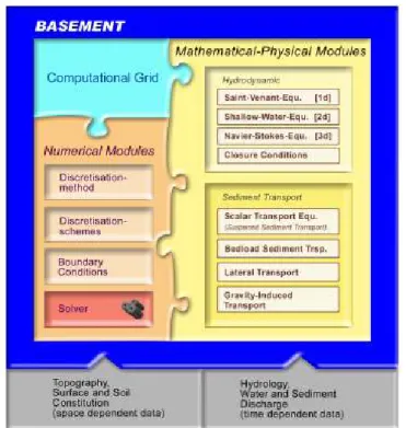
To reveal the “black box” of the numerical models, Figure 1.2 gives a graphical insight. The simulation tools of BASEMENT can be subdivided into three different parts:
• the mathematical-physical modules consisting of the governing flow equations • the computational grid representing the discrete form of the topography • and the numerical modules with their methods for solving the equations
In the next few chapters an overview of these modules is given. A more detailed description can be found in the reference manual.
1.4. Components BASEMENT System Manuals
1.4.1 Mathematical – Physical – Modules
The behaviour of the fluid hydraulics can be explained with physical models, namely the conservation of mass and momentum. Theoretically, it is possible to resolve the mathematical problem up to small scale phenomena like turbulence structures. In a natural problem however, it is mostly impossible to determine all boundary- and the exact initial conditions. Furthermore, the computational time needed to solve the full equation system is increasing very fast with higher spatial and temporal resolution. Therefore, dependent on the problem, simplified mathematical models are used.
In three dimensions, the flow and pressure distribution are completely described by the Navier-Stokes equations. These equations can only be solved numerically, as analytical solutions exist only for some strongly simplified problems. The 3-dimensional approach is only suitable for local problems, where turbulence phenomena and flow in all directions are essential for the results, e.g. the flow around bridge piers.
Assuming a static pressure distribution and neglecting the vertical flow components, the Navier-Stokes equations simplify to the 2-dimensional shallow water equations. This set of equations provides accurate results for the behaviour of water level and velocities in a plane. Turbulence effects cannot be resolved anymore but are accounted for by an artificial friction factor in the closure condition, which establishes a relation between flow velocity and shear stress. The shallow water equations are used for 2-dimensional flows like dam breaks, curved flow etc.
Reducing the spatial dimension once more results in the 1-D Saint-Venant equations. The main outputs of these equations are the water level and mean velocity in flow direction. This method is still in use for computing large river systems.
The computation of sediment transport is mathematically not as well developed as the hydrodynamic part. Theoretically, the movement of every single stone within the sediment could be computed by solving its equation of motion. However, this approach is yet numerically too expensive. Therefore, sediment transport and behaviour of the riverbed are computed using empirical formulas developed by river engineers. The computation of the sediment flux is physically not really correct, but proved to be accurate enough for a broad range of sediment transport problems. Usually, sediment transport occurs in the main flow direction. More sophisticated models consider also lateral phenomena within a curved flow.
Very small grain sizes are treated as suspended sediment load. Their behaviour can be computed by a physically scalar transport equation.
1.4.2 Computational Grid
1.4.2.1 The Meta Model
An important aspect of every computational task is the grid generation where the real world topography data is transformed into an internal computational grid on which the governing equations are solved. Independent of the discretization method, the construction of the computational grid has great impact on the accuracy of the results and on the computational time needed for the simulation or the numerical time step, respectively. Generally, a suitable mesh is dense at regions, where strong changes in the flow occur and
BASEMENT System Manuals 1.4. Components Element Node Edge Model Topography river and interpolated cross-sections DTM triangulated surface local coordinate system
„original“ Topography river cross -sections scattered points, elevation level curves river distance, national coordinate system
Grid Topology Structured 1 2 3 4 ... 2 3 4 Unstructured Discretization Methodology
control volumes (CV), flux over eges Finite Volume Method
(FVM) cell centred xi xi +1 cell vertex xi xi+1 xi -1 Numerical Model „Real World“ Model Meta Model
Figure 1.3 The Meta Model: fusion of “real world” data with abstract numerical considerations
1.4. Components BASEMENT System Manuals coarse in regions of lower interest. Additionally, the grid cells should not underlie strong deformations.
Usually, the raw real world data comes in form of river cross sections or geographic terrain models e.g. from a GIS. This elevation information has to be mapped onto a suitable mesh. There are two types of computational grids: structured and unstructured ones. Structured grids consist of quadrilaterals and can be mapped onto a Cartesian domain. They allow for simple data structures and efficient algorithms. The mesh generation is relatively simple and can even be done manually. However, structured meshes are somehow unhandy for the representation of arbitrary topography data. Unstructured grids are mostly composed of triangles and cannot be mapped onto Cartesian meshes. They usually need more complicated data structures but are highly flexible for automatic mesh generation in complex geometries. An unstructured grid is the most general case of a grid based discretization and is perfectly suitable for object oriented modelling. BASEMENT is built on unstructured grids.
The computational grid consists in general of cells (control volumes). In the software model, the mesh is based on three different objects:
• [node] the nodes – mass free points in relation to a coordinate system;
• [edge] the edges, which are defined by two nodes and define the place of information flux between two elements in Finite Volume Methods;
• [element] the elements, which are defined by several nodes and define the place of the physical variables, e.g. cell centered methods.
This data structure allows for similar treatment of 1-D and 2-D methods and schemes. As the difficulty of mesh generation occurs in many different computational tasks, a broad range of different triangulation techniques or mesh refinement methods can be found in the literature. Some of them are specially designed for a certain discretization scheme but can also be used elsewhere. As there is nothing such as an ideal or perfect mesh, the user is recommended to produce different grids and compare their behaviour to find the best solution. There are commercial tools available which can be used for the grid generation, e.g. SMS. However, the BASEMENT standard for grid representation (see Reference manual) also allows for self created meshes.
1.4.2.2 BASEchain : one dimensional model
In one dimension, an element consists of two nodes with known cross-section. With a cell-centred discretization, all variables – velocity, flow depth and cross-section geometry - are defined at the location of the nodes. The midpoint of the connecting line between two nodes defines the common edge of the two elements. The more nodes are known, the better the representation of the real world data, especially at regions with strongly curved watercourse.
1.4.2.3 BASEplane : two dimensional model
In two dimensions, an element consists of three nodes with a known ground elevation. Usually, this real world height information is not given exactly at the desired node
BASEMENT System Manuals 1.4. Components
Figure 1.4 Discrete Representation of the Topography within BASEchain
1.4. Components BASEMENT System Manuals
BASEMENT System Manuals 1.5. Simulation Procedure coordinates and therefore has to be interpolated. The primary variables are defined somewhere inside the element, e.g. the balance point. The fluxes between two elements are defined at their corresponding edges.
1.5
Simulation Procedure
The procedure to simulate a concrete problem setup is not unique. BASEMENT is coded using an object-oriented design which allows for flexibility and interchange ability concerning different application problems. The possible combinations are manifold. On the one hand, the governing equations may change dependent on simplifications or extensions of certain terms, use of sediment transport or pure hydraulics, etc. On the other hand, there are miscellaneous numerical methods, e.g. for time integration (implicit, semi-implicit, explicit) or computation of spatial fluxes. Therefore, the main variables of interest differ from one problem to the other. It is of great importance, to plan carefully each simulation approach to a certain problem. The most difficult and time-consuming part is not the simulation itself but the acquisition of all needed data (topography, boundary- and initial conditions) and a proper setup of this data. This section describes the main activities performed to execute a simulation with BASEMENT in a very general case. In most problems, only a part of them are being used.
1.5.1 Flow of main activities
1.5. Simulation Procedure BASEMENT System Manuals
BASEMENT System Manuals 1.5. Simulation Procedure
Figure 1.7 Flow of main activities, part II
Figure 1.8 Activity diagram generate computational mesh
1.5.2 Scenario Examples
Depending on the chosen scenario and on the available boundary conditions or i.e. topography data, the approach for a successful simulation differs from case to case. As there are different ways to reach a certain target, the following activity diagrams just present possibilities but not a strict guideline.
An important part is always the grid generation. Usually, the raw topography data needs a lot of treatments (manual correction, interpolation, adjustment of single elements, etc.) until a suitable computational mesh can be generated. Although programs for grid generation like SMS provide some powerful tools to manipulate mesh transformations, the user still has to retain an overview over the required steps leading to the final computational mesh.
The following activity diagrams show a possible procedure for different project scenarios.
1.5. Simulation Procedure BASEMENT System Manuals
Figure 1.9 Activity diagram Sediment balance in a river
1.5.2.1 Sediment balance in a river 1-D 1.5.2.2 Flood 1-D + 2-D
BASEMENT System Manuals 1.5. Simulation Procedure
Figure 1.10 Activity diagram Flood 1-D + 2-D
2
Simulation procedure
2.1
Run BASEMENT with graphical user interface (GUI)
The start and executing of the BASEMENT software is described in the part “Introduction and Installation” of this manual. Further details concerning the GUI of BASEMENT are explained in Section4.1.2.2
Run BASEMENT on Microsoft Windows
When running BASEMENT under Microsoft Windows operating system, the easiest way to start a simulation is by double clicking on the command file ending with “.bmc”. Otherwise the program can be executed choosing the “Run. . . ” command for the Windows “Start”-menu or by double–clicking the executable file in Windows Explorer. After running, BASEMENT will open the graphical user interface where the command file can be loaded and the simulation can be started.
BASEMENT creates an initialization file in the user’s HOME-directory ‘bm.ini’, which stores the present work directory and scenario name to ease the input procedure for repeated simulations of the same scenario.
According to the existence of a main control block, either BASECHAIN_1D or BASEPLANE_2D, the appropriate simulation will be carried out.
2.3
Run BASEMENT on Linux
BASEMENT runs as a console application without screen graphics output. On LINUX you open a console and type ‘BASEMENT_vX.Y’ (replace X.Y with current version number) to start the executable (if no environment variables have been set, change into your ‘bin’ directory of the installation path). After running, BASEMENT will open the graphical user interface where the command file can be loaded and the simulation can be started.
2.4. Run BASEMENT in batch mode BASEMENT System Manuals BASEMENT creates an initialization file (as a hidden file) in the user’s HOME-directory ‘.bm.ini’, which stores the present work directory and scenario name to ease the input
procedure for repeated simulations of the same scenario.
According to the existence of a main control block, either BASECHAIN_1D or BASEPLANE_2D, the appropriate simulation will be carried out.
2.4
Run BASEMENT in batch mode
Executing a simulation with BASEMENT normally opens the graphical user interface (GUI) and requires some input from the user, e.g. to select the model data and to confirm warnings generated by the program at the start and during run-time. But BASEMENT can optionally be started without any graphical interaction and without user input. This feature is especially useful if one or several models shall be run automatically via batch or script file.
But be aware that executing in batch mode requires special attention, since significant warnings may be suppressed without being noticed! It is recommended to study the generated ‘log-file’ after the simulation to check the program output for warnings which may have been generated during run time.
Executing in batch mode can be specified at the program start of BASEMENT using program arguments. The following list of program arguments is supported at the moment and can be specified in any order.
Table 2.1 List of program arguments. Command line arguments Description
- b BASEMENT is run in batch mode without manual
user input.
- f filename The file flag ‘-f’ and the space separated ‘filename’ argument specify the model filename which shall be executed. The filename must be the full path
including the name of the *.bmc-file. (Please note: no empty spaces are allowed to be part of the filename!) - version Display the version number of the BASEMENT
executable.
- h This help flag ‘-h’ displays all available command line arguments.
- doc This generates a reference documentation of all blocks and parameters in .html format.
-log [1-4] The number [1-4] defines the level of log output generated by BASEMENT.
BASEMENT System Manuals 2.5. Restart the simulation in BASEplane. . . Type the following line to execute the model ‘Scenario1.bmc’ in batch mode without user input.
BASEMENT_vX.X.exe –f d:\data\Scenario1.bmc -b
2.5
Restart the simulation in BASEplane from a given
solution
In 2D simulations with BASEplane an improved and enhanced method for the restart from existing solutions from old simulation runs was implemented. Such a ‘restart-file’ contains all relevant information and data which is needed for the continuation of an old simulation and therefore often needs a lot of disk storage. These data are now stored in a binary format to reduce the needs for disk storage and to obtain smaller files. For this purpose a standardized CFD format was chosen (CGNS – CFD General Notation System,
www.cgns.org). This standardized data format additionally can be edited and visualized by different programs and simplifies data exchange between different programs. (A simple Data Viewer for CGNS files is the adfviewer which can be found onwww.cgns.org). The restart from an old solution is possible for the hydraulic computations, bed load transport computations and suspended load computations.
Using this new file format the possibilities to continue a simulation from a given solution were enhanced. It is possible to continue a simulation not only from the last point in time of the old simulation run, but also from different times of the old simulation. This can be very helpful especially for large simulation runs with long durations. For example, if there was an error in the inflow hydrograph at a point in time, than the simulation can be restarted shortly before the time when the error occurred with a corrected hydrograph and without having to repeat the whole simulation from beginning.
3
Preprocessing
3.1
General
3.1.1 Requirement
The main purpose of the pre-processing activities is to define the project and the different scenarios, to prepare the available (topographic) input data and to put it in the format needed by the computational module as shown in the overview in Section1.1. Additionally, the choice of computational approaches and boundary/initial conditions has to be made.
3.1.2 Project / Scenarios
A project is defined for one region which is to be analyzed. Within a project, one or more scenarios can be embedded. To manage a project, it is therefore necessary to define which scenarios, files, and other elements belong to it. This includes the information where all these elements are stored and how they are connected to each other.
For the same project, several scenarios can be created. For each of them a simulation is executed. The different scenarios can vary regarding the computational mesh, other input data, the used approaches and the boundary conditions. In addition, type, location and time of the results to save have to be specified. The simulation can be done in 1, 2 or 3 dimensional computation or as a combination of them. The phenomena to be considered have to be chosen as well, as there are at the moment: dam break, bed load, suspended load, debris flow, mobile bed, erosion, collapse, pollutants etc.
3.1.3 Input data
As mentioned in the introduction, there are three main types of data to be provided for a simulation: topography, hydrology and sediment data. All data has to be transformed in a certain way to satisfy the input specifications of the main computation program. The precise specifications are available in the reference manual.
3.1. General BASEMENT System Manuals 3.1.3.1 Topography / Computational mesh
The most important, and most laborious to achieve, input is the retrieval and setup of the computational mesh. It is based on the real world topographic data. At the end of the pre-processing task, a grid in a defined shape and format is available for the simulation module.
This mesh can be generated in different ways. The topographical raw data may come from a cluster of points described by three dimensional coordinates, digitized contour lines, break line polygons or cross sections and probably is furnished in different file formats, which have to be interpreted and transformed. For a 2-D simulation, in a first step a TIN (Triangulated Irregular Network) has to be generated. Then this mesh has to be modified and refined in order to satisfy the special mesh qualities needed for stability of computation. For the 1-D model it might be necessary to interpolate cross sections or deduce cross sections from a DEM (digital elevation model).
3.1.3.2 Hydrologic data
At all boundaries of the mesh, hydrologic boundary conditions such as hydrographs or time series of water levels have to be provided. In the case of a simulation with sediment transport, also a sediment concentration in the water might be needed.
The choice of boundary data has to be made with care, considering the type of event being simulated. The data might be created especially for the wanted simulation hypothesis or be adapted from existing measured or statistical data. Some times, special manipulation of the data turns out to be necessary, for instance to omit discharges not relevant for sediment transport. Finally, again, the hydrologic data has to be put in the format wanted by the program.
3.1.3.3 Sediment data
Sediment data primarily comes from water sediment samples or surface samples like the line method. Possibly, a grading curve still has to be built from this raw data. Then the number of desired grain classes for the simulation has to be chosen and the characteristic grain classes need to be identified. Based on the grain distribution, other values like roughness or angle of rest may have to be calculated.
3.1.4 Boundary conditions
The boundary conditions define quantities at the margin of the computational region during the whole simulation time. These are typically hydrographs at the inflow boundary and water levels at the outlet boundary. In general, different special conditions can be applied by defining for instance the water level of a lake, weirs, steps, etc.
3.1.5 Source terms and local properties
For every mesh element, several characteristics can be specified, for example not flown through cells, mobile bed, bed load potential, k-value, roughness, shear stress or others.
BASEMENT System Manuals 3.2. Model input data Sources and sinks of water and/or sediments might be added within the computational region.
3.2
Model input data
3.2.1 Topographic data sources
The topographic raw data in the form of digital terrain information builds the fundamentals for grid generation and further numerical simulations using the BASEMENT software. In the case of 1-D simulation, the raw data consists of recordings of river cross-sections. In a 2-D or 3-D model, the raw data is built from point clouds, height contour lines or a digital terrain model (DTM).
Dependent on the assignment and its requirements, most of the raw data usually gets collected by experts. However, there are some extensive topographic models with different quality available, see e.g. the cross-sections database from the Federal Office for the Environment (BAFU) and high resolution terrain models from “swisstopo” or “Swissphoto AG”.
The next sections provide a short overview of different methods and data sources of data sources for topography and also hydrology and sediment. Most data sources in the next few sections are somehow related to Switzerland. Other regions and countries provide similar data – depending on the actual law.
3.2.1.1 Terrestrial data or surveying with differential GPS
Surveying or special engineering agencies provide terrestrial terrain data or terrain data obtained by differential GPS (DGPS) of the desired quality. A pure terrestrial recording is more expensive because at least two workers are needed in contrast to a DPGS scan, which can be done by one employee only.
The survey with GPS needs a certain visibility concerning the GPS satellites. The accuracy depends on the exactness of positioning for the reference point but usually lies in the range of a few centimetres.
The terrain data is delivered in different formats as e.g. xyz-coordinates or GEOBAU standard. Be sure to specify your claims on quality of the data as resolution, typical terrain deformations but also the desired data format when asking for a tender offer.
3.2.1.2 Official topographic survey
According to a decision of the Swiss federal assembly (“Einführung der amtlichen Vermessung” AV93), the bureau of land charge register provides digital cadastral data almost over the whole country (ca 80%) and data from the country’s information system (ca 30%).
The cadastral information is just of secondary use as the parcels are all flat. However, the ground plans of certain constructions and buildings may be helpful.
The data from the country’s information system can be used (with some additional work) for the definition of boundary conditions, e.g. data about floor cover types.
3.2. Model input data BASEMENT System Manuals The data format used for the AV93 act is called INTERLIS (Data exchange mechanism for “Landes-InformationsSysteme”).
3.2.1.3 Laser scanning
Essential factors for an accurate triangulation concerning topographic raw material are accuracy of position and height as well as the density of the measured points. Of special interest are therefore height model data taken by Airborne Laser Scanning (LIDAR) as e.g. provided by “swisstopo”. This method allows for a good data base within forests. Only in dense coniferous forest, the determination of the terrain model tends to be impossible. Of course, as with all measurements from the air, neither ground nor surface levels from water bodies can be obtained.
As the surface model generated from the LIDAR method distinguishes between terrain, buildings and vegetation, it provides a good starting point for further processing towards a numerical grid.
The federal office for topography (“swisstopo”) has commissioned Swissphoto AG to collect height data all over Switzerland for the identification of agricultural areas. However, this project is restricted to areas below 2000 m asl. For higher located zones (which could be relevant for debris flows), the data could be produced with reasonable costs. Until end of 2007 this project shall be finished.
“swisstopo” delivers their terrain data in two formats:
• DTM-AV raw: a point cloud with averagely 1 point per 2 m2
• DTM-AV grid2: an interpolated 2x2m mesh
The accuracy of position and height is about +/- 0.5 m. Additionally, “swisstopo” also works with 1x1m meshes which reach an accuracy below +/- 0.3 m.
For large areas and a high density of grid points, the amount of data is beyond the resources even of nowadays computing power. Therefore, there exists a variety of algorithms which eliminate all unnecessary points in a certain area that have no influence on the shape of the triangulation. This may reduce the amount of data by 10 – 60 %.
3.2.1.4 Sources and quality of data
One main factor for the quality of the results is the accuracy of the original topographic data. The accuracy varies depending on the objective of the recording, as well as on the recording methods. The accuracies of the most diffused methods are listed in Table 3.1.
Table 3.1 Accuracy of current measurement methods
Situation accuracy Height accuracy Observations Terrestrial +/- 2 cm (1) +/- 5 cm (1)
BASEMENT System Manuals 3.2. Model input data Situation accuracy Height accuracy Observations
GPS +/- 1-3 cm (1) +/- 1 cm (4) +/- 5 cm (1) At least 4 satellites Orthophoto +/- 2-3 cm (1) 0.2 – 0.3 ‰ of flying altitude (3) 3 cm with photo scale 1:2000 LiDAR +/-20-30 cm (2) open lea +/- 15-20 cm forest insecure (3)
Radar (InSAR) open lea +/- 20 cm (3)
(1) Gewässergeometrie, Landesanstalt für Umweltschutz Baden-Württemberg, Karlsruhe 1999.
(2) Swissphoto AG (verbal).
(3) Leitfaden Qualitätssicherung Photogrammetrie und DTM-Generierung, Konferenz der Kantonalen Vermessungsämter, 2000.
(4) GPS global positioning System, “swisstopo”.
The products which are directly available in Switzerland and their accuracies are listed in the following tables.
Table 3.2 Products offered by “swisstopo”
Product Density Source Format Accuracy
DHM25 Base Model DTM 35-1600 point /km2 1:25000 map Vectorized contour lines and contour lines in lakes, lake perimeters and spot heights, main alpine break lines (photogrammetric data) Arc View Shape- Files, DXF,GEN, BMBLT Mean error 1.5 to 3 meters depending on the regions DHM25 Matrix Model DTM 1600 point/km2 Interpolation of the Base Model on a 25x25m grid MMBLT, MMBL, AIGRID, XYZ, DXF, VRML
3.2. Model input data BASEMENT System Manuals
Product Density Source Format Accuracy
(1)DTM-AV raw (2)DTM-AV grid2 1 point for 2 m2 Based on official measurement with Lidar Airborne Laser Scanning(1) 2x2m grid interpolated from DTM-AV raw (2) ASCII , Interlis, others possible if requested Height accuracy +/-50 cm (1)DSM-AV raw (2)DSM-AV grid2 1 point for 2 m2 With buildings and vegetation (1) 2x2m grid interpolated from DSM-AV raw (2) ASCII , Interlis, others possible if requested Height accuracy 50 cm +/-150 cm for vegeta- tion
Table 3.3 Products offered by Swissphoto AG
Product Density Source Format Accuracy
DSM 10x10m, 20x20m,
50x50m
Photogrammetric interpretation of aerial photos from 1995/96 ASCII xyz or GRID Height accuracy: 3-5m midland and 7-10 mountains DEM LIDAR (on commission) 31000/(250x160m), spacing 1-1.3m Lidar Airborne Laser Scanning ASCII xyz, ASCII ArcInfo, . . . Height accuracy 30 cm
3.2.2 River related data sources
The following list provides some more Swiss data sources for real world problem modelling and boundary conditions.
River cross-sections: Primary use for 1-D models; also qualified for 2-D models to improve topography data within a rivers area. Terrestrial mapping, optimal quality and format according to the cross-section database of the Federal Office for Environment FOEN (formerly FOWG / bafu.admin.ch).
Terrain topography: Basic dataset for simulations with spatial (2- or 3-D) models. Optimal quality and format (ASCII x y z) as swisstopo DTM-AV / DOM-AV (New swisswide high resolution DTM/DOM based on laser scanning). (http://www.
swisstopo.ch/de/digital/dom.htm)
Surface texture and special buildings: Declaration of roughness coefficients, porosity and erosion resistance of surfaces; Optimal format INTERLIS-1, as e.g. DOM-AV or floor cover plans AV93 (generated by the cadastral register on demand of the cantons).
BASEMENT System Manuals 3.2. Model input data Sedimentological /geological data: Surface characterization of the riverbed (mostly using line samples), of the erosion capable underground (volume sampling or geological drilling) and of the flow induced transported material (grain size distribution from sieve analysis).
Possible data sources: geology of cantons, FOEN (formerly BWG), Nagra, in situ suspended load and bed load measurements.
The estimation of sedimentologic data and its analysis is surely the most time consuming part. At certain water bodies, a continuous monitoring of suspended load exist. However, the granulometric size distribution is seldom measured. Therefore, the bed load near the surface but also the suspended load often have to be estimated under certain assumptions or they will have to be measured.
Hydrological data: Temporal or stationary boundary conditions for the numerical model, e.g. inflow discharges, water levels and local sources or sinks.
Possible data sources: Hydrological data from the federal measuring facilities, specific rainfall-discharge models (e.g. IFU/ETHZ), retention models.
For larger water bodies within Switzerland (observed by the FOEN), time series and hydrographs are available online. Smaller watercourses are often not covered and need either a hydrologic model or new measuring/monitoring to determine the discharge.
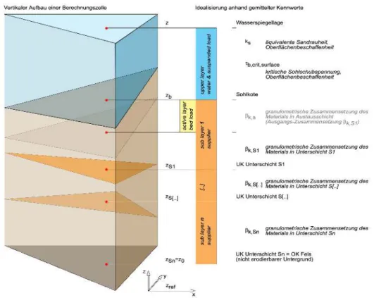
3.2.3 Characteristic quantities of riverbed
The numerical models used for the computation of hydraulic behaviour are always declared to be either 1-D (flow in direction of main flux / x-axis) and/or 2-D (horizontal, depth averaged flow field). However, the fundamental terrain topography is always three-dimensional. The spatial discretization of the transport equations is based in 1-D on cross-sections or in 2-D on an unstructured grid of mostly triangles. The vertical component consists of different layers separated by a planar joint face for both, 1-D and 2-D simulations.
The characteristic values are indicated relative to a joint surface (e.g. riverbed level) or to a layer (e.g. granulometric composition of bed material in layer S1). Their properties are represented in the balance point of the corresponding joint plane. This results in a simplified model of the layering for a computational cell. The characteristic data used in the model to describe the state and conditions of the surface are defined as followed: Position: Soil - properties =
zR: bottom elevation (bed level)
zSub : elevation level of the lower, closing joint plane of the
corresponding sublayer Subi(i∈1...n, withn = maximum
number of Sublayers)
z0 : elevation level of the lower joint face of sublayer Sn, which
finishes the model downwards, respectively describes the position of the non erodable underground.
(all variables are measured in [m.a.s.l.] or in [m] relative to a userdefined reference system) Attributes:
3.2. Model input data BASEMENT System Manuals
Figure 3.1 Visualization of the vertical setup for a computational cell within the models.
Vegetation− ground covering =
ks [m] : equivalent sand roughness based on Nikuradse:
description of the surface roughness (e.g. grass, sealed plane, etc.). (default value or derived by grain distribution of the first sublayer)
τB,crit [N/m2] : critical value for begin of sediment movement at
the surface, in the sense of a rised erosion constancy, e.g. by natural cover (default values)
Soil–properties =
βg,Subi [−] : mass fraction of theg
thgrain class relative to the
total mass of sublayer (default values according to the grain size distribution)
βg [−] : mass fraction of thegthgrain class relative to the
total mass of the active layer (possible default values according to line samples if available)
The listed attributes are mostly not completely determinable directly. For example, the equivalent sand roughness ks based on Nikuradse is an experimentally obtained value
for the flow resistance of different kind of surfaces. In the case of a more complex soil structure, ks may consist of several components. Its actual value has to be determined
by a calibration of the numerical model. The same holds true for the critical value τB,crit
which defines the beginning of movement at the soil surface. This value is affected by the character of the bed surface like natural cover or sealing (at farmlands). Without special conditions, the critical value can be estimated via the grain size distribution.
The mass fraction βg,Subi of grain class g in sublayer Subi has to be derived from an experimental grain size distribution using a sieve analysis. The material to be sieved may
BASEMENT System Manuals 3.2. Model input data come from a near surface sample take (e.g. by daggering) or a drill hole. The granulometric composition directly at the surface can be estimated by a line sample. Accordingly, the corresponding mass fractionsβg in the active layer can be determined.
3.2.4 Processing the raw data
It was shown in the previous sections that the numerical model needs some specific characteristic values which usually are not given directly by in situ measurements. Often, some experience in handling computational simulation models is necessary to reproduce the natural conditions in an adequate way and obtain realistic results.
3.2.4.1 Topography
The topographic raw data for 1-D or 2-D simulations comes in the form of cross-sections or by a digital terrain model (DTM). For a 1-D model, cross sections are mostly of accurate quality and need just few corrections and adaptations. However, most DTM’s serving as a base for a 2-D model need an elaborate revision because of the surface triangulation:
• the resolution of the DTM and the computational grid are not congruent (e.g. areas of lower interest shall have a coarse grid to reduce computational effort – the DTM usually has a uniform point density)
• the course of water bodies is not continuous or cross sections are not complete (e.g. data only available up to the water level)
• passages are not omitted (e.g. bridges)
• modelling and representation of buildings is not a priori known (e.g. height of buildings, retention volume, flow resistance)
• relevance of waste edges and artefacts are costly to determine (e.g. small walls, temporary dumpsites, hedgerows)
• etc.
The choice of software resources for processing the topographic raw data is huge, but often, these programs are somehow limited to specific applications and data formats. It is therefore recommended to specify the desired data format and resolution in advance to avoid unnecessary repetitions.
More detailed information about grid generation is given in the next chapter.
3.2.4.2 Hydrology
The hydrologic raw data for discharge and water levels usually has a non uniform resolution in time. Often, the measurements are indexed with date and time. For the simulation module, the time series have to be converted to a system with standard units (e.g. seconds). In an easy case, the converted data can directly be used as a boundary condition. The simulation module will then interpolate the desired values to the actual computational time.
3.2. Model input data BASEMENT System Manuals Further modifications may be necessary if e.g. just some time slots have to be simulated or if the main processes for a phenomenon like sediment transport occur at no more than a certain water discharge.
3.2.4.3 Grain size distribution
As mentioned earlier, the granulometric composition of the erodable material gets measured by a line sample or a sieve analysis and results in a grain size distribution (grain diameter versus weight percentages relative to the total sample weight). For the simulation, this distribution has to be discretized and desired grain classes have to be determined. Each grain class is defined by its medium diameter and has a percentage. The choice of the numbers of grain classes and thus the resolution of the material composition depends on the size of the problem and the computing power available. The classification of the grain diameters which represent a grain class strongly affects the transport behaviour of the whole material and the efficiency of the transport model.
It is recommended to run several simulations with one but also with more grain classes and to compare them.
3.2.5 GIS Interface
A geographic information system (GIS) as assistance for a numerical simulation model shall provide several data in best possible spatial and temporal resolution but not necessarily in a model inherent format. The data structures described in the following are just proposals. For all of them, one has to decide a priori whether the raw data shall be saved per se or in a processed form (raw data and pre-GIS-processed data).
3.2.5.1 Administration of geographical data
Generally, one distinguishes two kind of data types: matrix data (based on a uniform matrix, e.g. air taken pictures) and vector data (e.g. property borderlines).
Vector data serves for the visualization of the geometry and uses different data structures. Objects with simple geometry (see “OpenGIS Simple Feature Specifications”) are e.g. points, lines and polygons. For complex geometries (see “OpenGIS Geography Markup Language (GML)”), additional information as topology and other attributes (e.g. time) are required.
A further possibility to structure geographical data in a GIS is a splitting on different topic layers. Digital terrain models with height information are represented in a GIS either as TIN (triangulated irregular network) or as a GRID (structured mesh). With regard to numerical simulation models, the topology of a TIN or a GRID corresponds to unstructured resp. uniform computational grids.
3.2.5.2 Plane assignment for point data
In a GIS, real, area-related conditions are given in an idealized way. On the one hand, there is a limited number of attributes and on the other hand the values over the surface are averaged. Partially, the data base is just point wise available and just sparsely against resolution and process scales of numerical simulation models, e.g. at geological
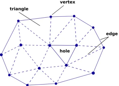
BASEMENT System Manuals 3.3. Grid generation
hole
edge vertex
triangle
Figure 3.2 Unstructured grid: Triangulation
probe holes. Therefore, the coarse values have to be extrapolated on the corresponding surfaces of the numerical grid. The determination of the corresponding surface, or i.e. the surrounding polygon, needs different geometric constructs as e.g. Dirichlet Tesselation (Voronoi-Polygons). Additionally, one should consider related information from superior
scales (e.g. geological maps with layering data and downcasts). 3.2.5.3 Interoperability and standard interfaces
To assure interoperability – meaning system independent communication – between different information systems, several norms for a standardized data representation exist. Examples are the “OpenGIS Geography Markup Language (GML)” or the norms used in Switzerland: INTERLIS (SN 612 030 / 612 031) and GEOBAU (SN 612 020).
3.3
Grid generation
3.3.1 Introduction
The numerical methods used for the approximation of differential equations needed in flow simulations are based on a discretization of the domain in simple small shapes. The complex of these elements forms a mesh. In BASEMENT, the finite volume method, being particularly valuable for fluid dynamics, is used.
To describe a topographic surface, the terrain data is often triangulated to allow a perspective representation of the topography. The result is a piece-wise linear interpolation of the surface. This triangulation can be used directly as mesh for simulations, as it permits to have the original data in the vertices of the initial grid and no interpolation is necessary. However, most of the time, the mesh has to be transformed somehow. Regions of high interest need some mesh refinement for higher accuracy and areas of lower interest are often coarsened to save computing power.
In numerical simulations, two types of meshes are used: structured and unstructured grids. Structured grids are simpler to use, but need an interpolation of the data to determine the
3.3. Grid generation BASEMENT System Manuals values at the desired vertex position if the input is an irregular point cloud. In addition, they are not sufficiently flexible to fit complex geometries.
Among unstructured meshes, the triangulated irregular networks (TIN) are most convenient because they fit the irregular distribution and complex geometry of the topography best. Furthermore, they allow for a rapid transition from small to large elements and the insertion and conservation of break lines. BASEMENT is built on unstructured grids.
The computational mesh consists of vertices, edges which connect the vertices and elements (control volumes) which are bounded by the edges.
The triangulation of terrain data is a special case of mesh generation, as the vertices do not only have a position in the coordinate system but also elevation information. This is a so-called 2,5 dimensional problem.
3.3.2 Topographical input data
The original terrain data typically has a very irregular distribution and a locally variable density. Data can be available in different shapes:
• A cloud of points (x, y, z) e.g. digital elevation model; • Polygons e.g. digitalized contour lines;
• PSLG (planar straight line graph) e.g. a DEM with addition of break lines. This is the most general case, in which the input is a set of vertices and non-crossing line segments that must be conserved in the triangulation.
Although the raw input data, e.g. from a point cloud, could be directly used as a grid, usually further transformations are performed to gain a suitable computational mesh. A suitable mesh is mainly defined by its quality.
3.3.3 Mesh quality
3.3.3.1 Shape of mesh elements
The shape of the elements of the meshes has an important effect on the applicability of numerical methods. Speed (due to convergence time), accuracy and stability of a simulation depend strongly on the quality of the employed mesh. Therefore, it is important to produce the best possible triangulation for the application.
Size, shape and number of the elements play an important role for the quality of the mesh. Possible characterizations of a triangulation, which can be optimized depending on the application, are:
• minimal angle • maximal angle
• maximum edge length • total edge length • maximum height
BASEMENT System Manuals 3.3. Grid generation
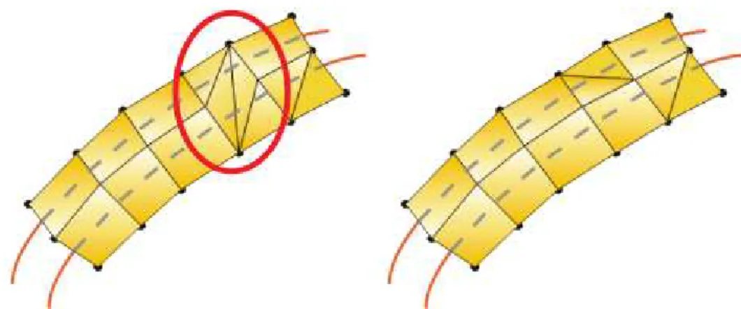
Figure 3.3 Left: ambiguous quadrilateral element with false break line; right: correct discretisation of the dyke crest.
• area of the triangle
• aspect ratio: ratio of the length of the longest side to the height (definition after Bern and Eppstein (1995), other similar definitions existent)
• aspect ratio: ratio of the circumference and the in-circle of a triangle
• roughness of the piecewise linear interpolation of a 2,5 D problem (The roughness of an interpolated surface can be measured e.g. by the Sobolev semi-norm)
The criteria which determine the quality of a mesh differ depending on the application (respectively partial differential equation) and the numerical method implemented. Also,
the possible optimization depends on the constraints given by the original data. It is recommended to avoid L-shaped overall areas (non convex hull) as such problems often lead to numerical instabilities in the concave corner.
In general, a height aspect ratio, very small angles and especially very large angles are considered as bad, as they lead to a poor numerical condition of matrices and increase the approximation error, which arises with the element size in general, as well. Big differences of size between neighbouring cell elements can have a negative influence on the numeric simulation too.
3.3.3.2 Ambiguous gradients
A further mesh quality criterion specific to meshes consisting of quadrilateral elements, or meshes with mixed element types, is the problem of ambiguous gradients. Quadrilateral elements are defined by four nodal points. These nodes ideally have elevations which guarantee that the four nodes lie within a plane. But in case of strongly varying terrain topographies, a bad placement of quadrilateral elements can lead to situations where this is not the case. Such elements are deformed and have an ambiguous gradient. Figure3.3
illustrates a quadrilateral element with ambiguous gradient which is situated across a river dyke.
In such situations a splitting of the quadrilateral element into two triangles becomes necessary. The selection of the correct break line within the quadrilateral element (here, along the dyke crest) must usually be done manually according to local topography. To
3.3. Grid generation BASEMENT System Manuals a) b) B A D C C D A B
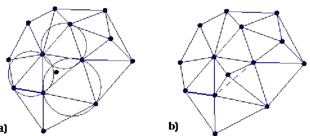
Figure 3.4 a) Empty circle criterion satisfied. b) Empty circle criterion not satisfied
facilitate this task, most grid generating tools (e.g. SMS) offer special features for detecting quadrilateral elements with ambiguous gradients in the mesh.
3.3.4 Issues on triangulation
Mesh triangulation and grid refinement play an important role in almost every numerical simulation. Therefore, a lot of different techniques have been developed to achieve suitable computational meshes. The user is basically free to use any tool or method which generates a mesh of accurate quality out of the raw data. This section shall give a short overview on some popular triangulation methods.
BASEMENT does not provide an automated routine for mesh generation. Therefore the plugin BASEmesh for the free and open source geographic information system (GIS) software Quantum GIS (QGIS) was developed (see Section3.3.5).
3.3.4.1 Delaunay triangulation and constrained Delaunay triangulation The Delaunay triangulation is one of the most employed triangulation methods because it optimizes several quality criteria: It maximizes the minimal angle and minimizes the maximum containment circle radius, the maximum enclosing circle radius and the roughness of a piecewise-linear interpolation. It also provides good results regarding the minimization of the maximum angle, but it does not find a global optimum in this case.
A Delaunay triangulation has the following properties. It • is the straight line dual of the Voronoi diagram; • is unique;
• respects the circumcircle criterion;
The circumcircle criterion is respected if the circumcircle of every interior triangle does not contain other points.
This corresponds to say that if ABC + CDA < 180° the empty circle criterion is satisfied. • respects the edge circle property: for each edge exists some point-free circle which
passes through the end points;
• respects the neighbour property: an edge formed by joining a vertex to its nearest neighbour is an edge of the triangulation.
BASEMENT System Manuals 3.3. Grid generation b) B A D C a) B A D C constrained edges
Figure 3.5 a) edge circle criterion. b) empty circle criterion
3.3.4.1.1 Constrained Delaunay triangulation (CDT)
The terrain data is sometimes provided in the shape of a PSLG as it contains break lines which must be conserved as edges in the triangulation. In this case, the constrained Delaunay triangulation can be used.
For the definition of a constrained Delaunay triangulation the notion of visibility of a point is needed: In a PSLG domain P a point D is visible to a point C if the open line segment CD lies within the domain and does not intersect any edges or vertices of P. Point D is visible to CB if it is visible to some point on CB.
For the CDT the edge circle and the empty circle criterion are modified as follows: • Edge circle: for each edge a circle passing through its end-points containing no other
point of the domain visible to the edge exists;
• Empty circle: the circumcircle of every triangle contains no points visible to points inside of the triangle.
3.3.4.1.2 MinMax triangulation
The MinMax triangulation minimizes the maximum angle. It has proven to be very useful in CFD (Barth, 1994).
3.3.4.1.3 Data dependent triangulation
A data dependent triangulation can be used for a 2.5 d problem. Its aim is to find the best triangulation under data dependent constraints, by minimizing a local cost function of a piece-wise interpolation. Two examples of local cost functions are described in (Barth, 1994).
3.3.4.1.4 Steiner triangulation
A Steiner triangulation is a triangulation in which extra points are added to the original data to improve the quality of the mesh. The additional points are called Steiner points. The number of Steiner points must be limited, limiting also the quality of the mesh.