Integer Factorization

(1)

Integer Factorization

Per Leslie Jensen<[email protected]>

Master Thesis

D I K U

Department of Computer Science University of Copenhagen

(2)

(3)

Abstract

Many public key cryptosystems depend on the difficulty of factoring large integers.

This thesis serves as a source for the history and development of integer factorization algorithms through time from trial division to the number field sieve. It is the first description of the number field sieve from an algorithmic point of view making it available to computer scientists for implementation. I have implemented the general number field sieve from this description and it is made publicly available from the Internet.

This means that a reference implementation is made available for future developers which also can be used as a framework where some of the sub algorithms can be replaced with other implementations.

(4)

(5)

4.1.2 The Theory . . . 25 4.2 RSA . . . 26 4.2.1 Correctness . . . 28 4.2.2 Formalizing RSA . . . 28 4.2.3 RSA Variants . . . 29 4.2.4 Security . . . 32 4.3 Discrete Logarithms . . . 37 4.3.1 Introduction . . . 37 5 Factorization Methods 41 5.1 Special Algorithms . . . 41 5.1.1 Trial division . . . 42 5.1.2 Pollard’sp−1method . . . 43 5.1.3 Pollard’sρmethod . . . 44

5.1.4 Elliptic Curve Method (ECM) . . . 45

5.2 General Algorithms . . . 47

5.2.1 Congruent Squares . . . 47

(6)

CONTENTS

5.2.3 Quadratic Sieve . . . 50

5.2.4 Number Field Sieve . . . 52

5.3 Factoring Strategy . . . 55

5.4 The Future . . . 55

5.4.1 Security of Public Key Cryptosystems . . . 55

5.4.2 Factoring in The Future . . . 56

6 The Number Field Sieve 57 6.1 Overview of the GNFS Algorithm . . . 57

6.2 Implementing the GNFS Algorithm . . . 59

6.2.1 Polynomial Selection . . . 59 6.2.2 Factor Bases . . . 61 6.2.3 Sieving . . . 62 6.2.4 Linear Algebra . . . 64 6.2.5 Square Root . . . 66 6.3 An extended example . . . 67

6.3.1 Setting up factor bases . . . 68

6.3.2 Sieving . . . 69 6.3.3 Linear Algebra . . . 70 6.3.4 Square roots . . . 73 7 Implementing GNFS 75 7.1 pGNFS - A GNFS Implementation . . . 76 7.1.1 Input/Output . . . 77 7.1.2 Polynomial Selection . . . 77 7.1.3 Factor Bases . . . 77 7.1.4 Sieving . . . 78 7.1.5 Linear Algebra . . . 78 7.1.6 Square Root . . . 78 7.1.7 Example of Input . . . 79 7.2 Parameters . . . 79

(7)

CHAPTER

1 Preface

“Unfortunately what is little recognized is that the most worthwhile scientific books are those in which the author clearly indicates what he does not know; for an author most hurts his readers by concealing difficulties.”

- Evariste Galois(1811-1832)

In 1801 Gauss identifiedprimality testing and integer factorization as the two most fundamental problems in his“Disquisitiones Arithmeticae”[29] and they have been the prime subject of many mathematicians work ever since and with the introduction of public key cryptography in the late 1970’s it is more important than ever.

This thesis is a guide to integer factorization and especially the fastest gen-eral purpose algorithm known:the number field sieve. I will describe the num-ber field sieve algorithm so it can be implemented from this description. To convince the reader I have implemented the algorithm from my description and have made the implementation public available on the Internet1so it can be used as a reference and maybe be improved further by anyone interested. The target reader is a computer scientist interested in public key crypto-graphy and/or integer factorization. This thesis is not a complete mathemat-ical breakdown of the problems and methods involved.

Even before Gauss, the problem of factoring integers and verifying primes were a hot topic, but it seemed intractable and no one could find a feasible way to solve these problems and to this day it still takes a large amount of computational power.

Till this day the problem of factoring integers is still not solved, which means there is no deterministic polynomial time algorithm for factoring inte-gers. The primality testing problem has just recently been solved by Agrawal, Kayal and Saxena[4].

Integer factorization has since the introduction of public key cryptosys-tems in 1977 been even more important because many cryptosyscryptosys-tems rely on the difficulty of factoring integers (large integers). This means that a very

(8)

CHAPTER 1. PREFACE

fast factoring algorithm would make for example our home banking and en-crypted communication over the Internet insecure.

The fastest known algorithm for the type of integers which cryptosystems rely upon is thegeneral number field sieve, it is an extremely complex algorithm and to understand why and how it works one needs to be very knowledge-able of the mathematical subjects of algebra and number theory.

This means that the algorithm is not accessible to a large audience and to this point is has only been adopted by a small group of people who have been involved in the development of the algorithm, that is: until now. . .

This thesis has the first algorithmic description of all the steps of the num-ber field sieve and it has resulted in a working implementation of the algo-rithm made publicly available.

The reader should know that it is a large task to implement all the steps from scratch, and here you should benefit from my work by having a refer-ence implementation and maybe start by trying to implement a part of the algorithm and put it into my framework. My implementation is probably not as fast and optimal as it could be but it is readable and modular so it is not to complex to interchange some of the steps with other implementations.

The implementation here has been developed over several months but it helped the understanding of the algorithm and have given me the knowledge to write the algorithms in a way so a computer scientist can implement it without being a math wizard.

The thesis consists of the following Chapters:

Chapter 2 gives the fundamental algebra for the rest of the paper, this Chapter can be skipped if you know your algebra or it can be used as a dic-tionary for the algebraic theory used.

In Chapter 3 I will take a trip trough the history of integer factorization and pinpoint the periods where the development took drastic leaps, to un-derstand the ideas behind todays algorithms you need to know the paths the ideas has travelled on.

The motivation for this paper is the link to cryptography and in Chapter 4 I will give an introduction to public-key cryptography and take a more detailed look on the RSA scheme, which is based on the difficulty of factoring integers and it is still the most used public-key cryptosystem today.

In Chapter 5 I will take a closer look at some of the algorithms mentioned in Chapter 3 and describe the algorithms leading to the number field sieve.

The main contribution in this paper is Chapter 6 and 7. In Chapter 6 I will describe the number field sieve algorithm step by step, and write it on algorithmic form usable for implementation. In Chapter 7 I will describe my implementation of the number field sieve, and give some pointers on implementation specific issues of the algorithm.

Acknowledgments

I would like to thankStig SkelboeandJens Damgaard Andersenfor taking the chance and letting me write this paper.

(9)

I am grateful for valuable help fromProf. Daniel J. Bernsteinwith the square root step.

Thanks to my parents and friends for supporting me through the long pe-riod I have worked on this, and for understanding my strange work process. Thanks toBue Petersen for helping with the printing and binding of this thesis.

Special thanks toJacob Grue Simonsenfor valuable discussions on- and off-topic and for proofreading the paper.

And a very special thanks to Katrine Hommelhoff Jensen for keeping me company many a Wednesday and for keeping my thoughts from wandering to far from the work at hand.

Per Leslie Jensen October 2005

(10)

(11)

CHAPTER

2 Mathematical Prerequisites

“God made the integers, all else is the work of man.”

- Leopold Kronecker(1823-1891)

The main purpose of this chapter is to present the algebra and number theory used in this paper.

The theorems are presented without proofs. For proofs see [5] and [69]. The reader is expected to have some insight into the world of algebra, con-cepts like groups and fields are refreshed here, but the theory behind should be well known to the reader. For a complete understanding of the inner work-ings of the algebra, a somewhat deeper mathematical insight is needed.

If you have a mathematical background this chapter can be skipped.

2.1 The Theory of Numbers

In all branches of mathematics the building blocks are numbers and some basic operations on these. In mathematics the numbers are grouped into sets. The number sets used in algebra are, for the biggest part, the set of integers, denoted Z, the set of rational numbers, denotedQ and the set of complex numbers, denotedC.

Other sets of great interest includes the set of polynomials with coefficients in the three above mentioned sets.

We will now take a look at some of the properties of these sets. 2.1.1 The SetZ

The set of integers (. . . ,−2,−1,0,1,2, . . .), denotedZ, has always been the subject for wide and thorough studies by many of the giants in the history of mathematics.

Many of the properties ofZare well known and used by people in every-day situations, without thinking about the underlying theory.

I will now take a look at the more intricate properties ofZthat consitute the foundation for most of the theory used in this thesis.

Prime numbers are the building blocks of the set Z, this is due to the unique factorization property which leads tothe fundamental theorem of arith-metic.

(12)

CHAPTER 2. MATHEMATICAL PREREQUISITES

Definition 2.1 Greatest Common Divisor (GCD)

Greatest Common Divisor ofa, b∈Z, denotedgcd(a, b), is the largest positive number,c, so thatc|aandc|b

Definition 2.2 Prime number

An integera >1is called a prime number if∀b∈_Z, b < a : gcd(a, b) = 1

Definition 2.3 Relative prime

Two integersa, bare said to be relatively prime ifgcd(a, b) = 1

Theorem 2.1 Fundamental Theorem of Arithmetic

Let a ∈ _Z and a > 1 then a is a prime or can be expressed uniquely as a

product of finitely many primes.

The next definition with the accompanying lemmas are the work ofEuler, and they help us get toEuler’s theorem andFermat’s little theorem.

Leonhard Euler

(1707-1783) is without comparison the most productive mathematician ever. He worked in every field of mathematics and in the words of

Laplace:“Read Euler, Read Euler, he is the master of us all´´. For a view of the man and his mathematics, see [24]. Pierre de Fermat (1601-1665) is considered to be the biggest ”hobby“ mathematicians of all times, he was a lawyer of education but used his spare time on mathematics.Fermat’s last theoremis one of the most famous theorems ever, it remained unproven for more than 300 years. The story ofFermat’s last theoremis told beautifully in [70].

Definition 2.4 The Euler phi function

Letnbe a positive integer. φ(n)equals the number of positive integers less than or equal ton, that are relative prime ton.

Lemma 2.1 Ifpis a positive prime number, thenφ(p) =p−1

Lemma 2.2 Forpandqdistinct primes,φ(pq) = (p−1)(q−1)

Lemma 2.3 Ifpis a prime andkis a positive integer, thenφ(pk) =pk−pk−1

Lemma 2.4 Ifn > 1has prime factorizationn=pk1

1 ·p k2 2 · · ·pkrr, thenφ(n) = (pk1 1 −p k1−1 1 )(p k2 2 −p k2−1 2 )· · ·(pkrr−pkrr−1)

Lemma 2.5 ais an integer andp6=qare primes andgcd(a, p) = gcd(a, q) = 1 thena(p−1)(q−1) ≡1 (modpq)

Theorem 2.2 B-smooth

Ifnis a positive integer and all its prime factors are smaller thanB thennis calledB-smooth.

By now we have the theory behind Euler’s Theorem and Fermat’s little theorem, and these can now be stated.

Theorem 2.3 Euler’s Theorem

Ifnis a positive integer withgcd(a, n) = 1, thenaφ(n)≡1 (modn)

Theorem 2.4 Fermat’s little theorem

(13)

2.2. GROUPS

2.1.2 Polynomials inZ,QandC

In the previous section we saw some of the properties of the setZ, especially the unique factorization property and the theory of irreducibility and prime numbers.

Now we turn our attention to polynomials, recall that a polynomial is an expression of the forma0+a1x+a2x2+· · ·+amxmfor somem∈Zand the coefficientsai ∈ Z,Qor C. And a lot of the properties ofZ is applicable to polynomials with coefficients inQorC.

Let us take a look at irreducibility and primes in regards to polynomials.

Definition 2.5 Divisibility inQ[x]

Letf, g∈_Q[x].f is adivisorofg, denotedf |g, if there existsh∈_Q[x], such thatg=f h. Otherwise we say thatf is not adivisorofgand writef -g.

Definition 2.6 Irreducibility and primes inQ[x]We give a classification of the elements inQ[x]. An element inf ∈Q[x]is one of the following

• f = 0and is called the zero polynomial

• f|1and is called aunit

• f is calledirreducibleiff =gh, g, h∈_Q[x] ⇒g orhis aunit

• f is calledprimeiff =gh, g, h∈Q[x]andf|gh⇒f|gorf|h(or both) • otherwisef is calledreducible

f, g ∈_Q[x]is calledassociatesiff =guwhereuis a unit.

2.2 Groups

Until now we have looked at elements from sets, and then applied opera-tions to them, both addition and multiplication. But when we look at ele-ments from a set and only are interested in one operation, then we’re actually looking at agroup.

AgroupGis a set with an operation◦which satisfies

• Theassociativelaw:

∀a, b, c∈G : (a◦b)◦c=a◦(b◦c)

• Existence ofneutraloridentityelement:

∃e∈G∀a∈G : e◦a=a◦e=a

• Existence ofinverses:

(14)

Definition 2.7 Abelian group A groupGis calledAbelianif

∀a, b∈G : a◦b=b◦a

Definition 2.8 Order of group

The order of groupG, denotedkGk, is the number of elements inG

A finite group is a group with a finite order. Unless otherwise stated the groups we are working with are finite.

Definition 2.9 Order of group element

The order of an elementg ∈ G, denotedkgk, is the smallest numberasuch thatga =e, ifadoesn’t exist thenghasinfiniteorder

Definition 2.10 Cyclic group

If there exists an elementg ∈ G, whereGis a group, andGcan be written

asG =< g >= (g, g1, g2. . .), then we say that Gis a cyclic group andgis a

generator forG

Corollary 2.1 Any groupGwith prime order is cyclic

An example of a group areZwith+as operator, this group is also Abelian. An example of a cyclic group is the multiplicative subgroupZ∗nofZn, which

contains elements that are relative prime withn,Z∗nis also finite.

Definition 2.11 Subgroup

His a subgroup ofG, if it contains a subset of the elements ofGand satisfies the 4 requirements of a group. It must at least contain the neutral element fromG. The order of the subgroupHhas to be a divisor of the order ofG.

Definition 2.12 Normal subgroup

LetH be a subgroup of a groupG. ThenH is a normal subgroup ofG, de-notedHG, if for allx∈G

xHx−1 =H

2.3 Mappings

A mappingσ :G7→Htakes an elementg∈Gand maps it toσ(g)∈H. Mappings can be defined for groups, fields and rings.

Definition 2.13 Homomorphism

A mappingσ : G 7→ H is called ahomomorphism, if it mapsG toH and preserves the group operation, i.e. for all g1, g2 ∈ G we have σ(g1g2) =

(15)

2.4. FIELDS AND RINGS

Definition 2.14 Isomorphism

A mappingσis called anisomorphism, if it is a homomorphism and is bijec-tive.

If an isomorphism exists between two groups they are calledisomorphic.

Definition 2.15 Automorphism

A mappingσis called anautomorphism, if it is an isomorphism and mapsG

toG.

A useful theorem, using isomorphism isThe Chinese Remainder Theo-rem, which is very helpful when working with finite groups of large order.

Theorem 2.5 The Chinese Remainder Theorem

If n = n1n2· · ·nm where allni’s are pairwise relatively prime, that is∀0 <

i < j ≤m: gcd(ni, nj) = 1then

Zn∼=Zn1×Zn1· · · ×Znm

2.4 Fields and Rings

One of the most important building blocks in abstract algebra is a field. A field is a setFwith the following properties

• (F,)is a multiplicative group • (F,⊕)is an Abelian group

When we look upon the properties for a field, we can see that the set of rational numbersQis a field, and so isC. One of the fields of great interest for cryptography over the years is the fieldZ/Zpof integers modulo a prime numberp, which is denotedFp.

Another interesting property of a field is that we can use it to create a finite group, if we have the field Fp = Z/Zp, we can create the group G = F∗p = (Z/Zp)∗, which is the group of integers relatively prime withp(the set

1, . . . , p−1) and with multiplication modulopas operator.

Often these properties are not fulfilled and therefore there is another strong object in abstract algebra, and that is aring.

AringFis a set with all the same properties as a field, except one or more of the following properties are not fulfilled:

• multiplication satisfies commutative law

• existence of multiplicative identity1

• existence of multiplicative inverses for all elements except0

(16)

Definition 2.16 Ring homomorphism

LetRbe a ring with operations+and·and letSbe a ring with operations⊕

and. The mapθ:R →Sis aring homomorphismfrom the ringR,+,·to the ringS,⊕,if the following conditions are true for alla, b∈R:

1. θ(a+b) =θ(a)⊕θ(b) 2. θ(a·b) =θ(a)θ(b)

Definition 2.17 Characteristic of field

The characteristicp of a fieldF, is an integer showing how many times we have to add the multiplicative identity1 to get 0, if this never happens we say thatFhas characteristic0.

Definition 2.18 Order of a field

The ordernof a field is the number of elements it contains.

Definition 2.19 Finite Field

A field is calledfiniteif it has a finite number of elements, i.e. a finite order.

Definition 2.20 A field Fis algebraically closed if every polynomial p ∈ F[x] has roots inF.

Carl Friedrich Gauss

(1777-1855) is considered to be one of the greatest mathematicians ever, he worked on algebra and number theory. And a major part of his work was a large publication on number theory in 1801[29].

Definition 2.21 Field Extension

Eis called an extension field of a fieldF ifFis a subfield ofE.

A field can be extended with one or more elements which results in an extension field. This is normally done with roots of a polynomial. Qcan for example be extended with the roots of the polynomialt2−5, this would be denoted Q(

√

5). Q( √

5)is the smallest field that contains Qand √

5 hence must contain all the roots oft2−5.

An extension with a root from a given polynomial is called aradical exten-sion.

A polynomialf(t)is said to split over the fieldF, if it can be written as a product of linear factors all fromF. In other words: all off(t)’s roots are inF.

Definition 2.22 Splitting field

Fis a splitting field for the polynomial f over the field GifG ⊆F, andFis the smallest field with these properties.

From the definition above it is clear that the splitting fieldGoff over the fieldFequalsF(r1r2 . . . rn), wherer1. . . rnare the roots offinF.

The next few theorems appear to belong in Section but they are used on elements from fields, so it is justified to have them here instead. The reci-procity laws are considered among the greatest laws in number theory and Gausseven called them the golden theorems. For a very thorough look at the history and theory of reciprocity laws see [38].

(17)

2.5. GALOIS THEORY

Definition 2.23 Quadratic Residue

A integer n is said to be quadratic residue modulop if nis a square in Fp,

p >2, otherwise it is called a non-residue

Definition 2.24 The Legendre symbol

Letabe an integer andp >2a prime. Then theLegendresymbol(a_p)is defined as a p =    0, if p|a

1, if a is a quadratic residue mod p

−1, if a is a non-residue mod p

Definition 2.25 The Jacobi symbol

Letabe an integer andnan odd composite number with prime factorization

n =pα1

1 ·p

α2

2 · · ·pαmm. Then theJacobisymbol(an)is defined as the product of

theLegendresymbols for the prime factors ofn

a n = a p1 α1 · a p2 α2 · · · a pm αm

A note on the last two definitions. In typographic terms the Jacobi and Legendre symbols are the same, but remember that they are not the same. Legendreis modulo a prime andJacobiis modulo a composite.

The reader have probably noticed that none of these symbols works for quadratic residues modulo 2. This is because 2 is a special case and all num-bers on the form8n+ 1and8n−1forn∈_Zare quadratic residues modulo 2.

2.5 Galois Theory

In the nineteenth century, the greatGaloisbrought many interesting ideas to the algebraic society. Although many of the ideas were not accepted right away, his genius was recognized years later and today he is considered to be

one of the biggest algebraists ever. Evariste Galois

(1811-1832)had ideas which expanded algebra to what it is today. His life is one of the biggest tragedies in all of mathematical history. For a look into the life ofGaloistake a look at the excellent book [63].

Going through all the ideas and theory developed by the young Galois deserves a couple of papers by itself and is out of the scope of this paper. For a complete look into the work ofGaloisthe reader should turn to [6] and [73]. We will only take a look on some of the main ideas ofGaloisand the theory needed later in this paper. This is especially the concept ofGalois Groupsand Galois fields.

In the last sections we have seen how a field can be extended by using elements like roots in a polynomial.Galoistook the concept of field extensions and cooked it down to the core elements.

Definition 2.26 Galois group

LetKbe a subfield ofF, the set of all automorphismsτ inF, which are such thatτ(k) =kfor allk∈K, forms a group, called the Galois group ofF over

(18)

As a consequence ofGalois’ work, it became clear that all finite fields con-tainspn elements, where p is a prime andn some integer. These fields can all be constructed as a splitting field fortn−toverZp. This discovery is the

reason for naming finite fields after the greatEvariste Galois.

Definition 2.27 Galois Field

The finite fieldFnwithnelements, wheren=pmfor some primep, is written

GF(n).

The definition of a Galois Field adds another name for a finite field, so we actually have three names for a finite field: Zp,Fp andGF(p) in this thesis a

finite field is denotedGF(p).

Definition 2.28 Characteristic of GF(pn) The characteristic of a Galois FieldGF(pn), isp

Although the most known terms are Galois group and Galois Field,Galois’ main work was on the theory of radical extensions and solvable groups.

Definition 2.29 Solvable group

A group is called solvable if it has a finite sequence of subgroups 1 =G0⊆G1 ⊆ · · · ⊆Gn=G

such thatGiGi+1andGi+1/Giis Abelian fori= 0, . . . , n

Theorem 2.6 Let F be a field with characteristic 0. The equation f = 0 is solvable in radicals if and only if the Galois group off is solvable.

Although some of these definitions looks simple, they are very hard to work with. One of the computational difficult subjects in mathematics is solv-ing theInverse Galois Problem, that is verifying that a given group is a Galois group for some polynomial in a field extension. This is not relevant to this thesis, but the interested reader should take a look at [34].

2.6 Elliptic Curves

Elliptic curves is a branch of algebra which has received a lot of attention over the last couple of decades. The reason for algebraists’ interest in elliptic curves is that the set of points on an elliptic curve along with a special opera-tion can be made into a group. The general theory of elliptic curves is beyond the scope of this paper, but we will take a look at some of the theory of elliptic curves, so we can illustrate how to create groups based on elliptic curve.

For a more comprehensive treatment of the theory of elliptic curves, the reader should turn to [69], [8],[42] or [27] and the more recent publication [31], which is the most comprehensive guide I have ever read, to the imple-mentation issues of elliptic curves.

(19)

2.6. ELLIPTIC CURVES

2.6.1 Introduction

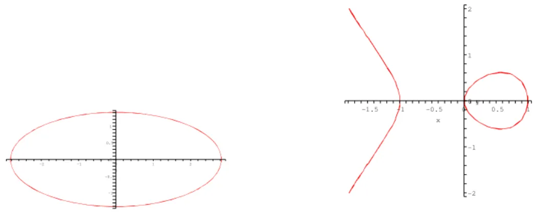
Elliptic curves should not be confused with ellipses, even though they share the same name. Elliptic curves are the result of a special kind of functions, namely the elliptic functions.

y 0.5 1 0 -0.5 -1 x 2 1 0 -2 -1 y 1 2 0 -2 -1 x 0.5 0 1 -0.5 -1.5 -1

Figure 2.1: An ellipse is shown on the left and a projection of the elliptic curve:y2+x3−xon the right

Elliptic functions have been studied by many of the great mathematicians through history, especially the work of Galois[28] and Abel[2] in this area is notable.

For mathematicians, an elliptic function is a meromorphic function1 de-fined in the complex plane and is periodic in two directions, analogous to a geometric function which is only periodic in one direction. You can just consider elliptic functions as being polynomials in 2 variables.

2.6.2 The Weierstraß Form

Karl Theodor Wilhelm Weierstraß (1815-1897) One of the pioneers on hyperelliptic integrals. He taught prominent mathematicians like Cantor,Kleinand Frobeniusto mention a few.

Elliptic curves are often written on the Weierstraß formalthough there exists other equations which can be used like theLegendre equationandquartic equa-tion. In this paper we will use the Weierstraß equation to describe elliptic curves, because the theory we need are best described in the Weierstraß form.

Definition 2.30 Generalized Weierstraß equation LetKbe a field. An equation on the form:

y2+a1xy+a3y=x3+a2x2+a4x+a6 ,

withai∈K, is called the generalizedWeierstraß equationoverKin the affine

plane2.

1_A_{meromorphic function}_{is a single-valued function that is analytic in all but possibly a finite}

subset of its domain, and at those singularities it must go to infinity like a polynomial, i.e. the singularities must be poles and not essential singularities.

2_{For a field}

Fn, theaffine planeconsists of the set of points which are ordered pairs of

(20)

In the Weierstraß form, thexandy cover a plane, and they can belong to any kind of algebraic closure.

Interesting properties of a Weierstraß equation is its discriminant∆and itsj-invariant j. In most literature on the subject, it is common practice to use a few intermediate results to express∆andj, these are

b2 = a21+ 4a2

b4 = 2a4+a1a3

b6 = a23+ 4a6

b8 = a21a6+ 4a2a6−a1a3a4+a2a23−a24

c4 = b22−24b4

The discriminant andj-invariant can then be written as ∆ = −b2₂b8−8b43−27b26+ 9b2b4b6 j = c 3 4 ∆ Definition 2.31 Singularity

A pointpis a called asingular point, if the partial derivatives of the curve are all zero at the pointp. Singular points could for example be

• acuspwhich is a point where the tangent vector changes direction

• a cross intersection point where the curve ”crosses” itself

Definition 2.32 A curve is calledsingularif it has one or more singular points, otherwise it is callednon-singular.

Theorem 2.7 If a Weierstraß equation has discriminant∆ = 0then it is singu-lar.

These theorems makes it possible to define what an elliptic curve is: A non-singular Weierstraß equation defines an elliptic curve. When using the term: “elliptic curveEover a fieldK” I mean the solutions inKto the curve’s Weierstraß equation the set of which is denotedE/K.

Definition 2.33 Two elliptic curves defined over the same base field are iso-morphicif theirj-invariant are the same.

When using an elliptic curve over a Galois Field, we can estimate the num-ber of points by usingHasse’s theorem, which was originally conjectured by Artin in his thesis for general curves and proved later by Hasse for elliptic curves. A proof can be found in [69].

(21)

Theorem 2.8 Hasse’s Theorem

Given a Galois FieldGF(q), the number of rational points on the elliptic curve

E/GF(q)is denoted|E/GF(q)|:

q+ 1−2√q ≤ |E/GF(q)| ≤q+ 1 + 2√q

Definition 2.34 Trace of Frobenius

For an elliptic curveEoverGF(q), thentdefined as

t=|E/GF(q)| −q−1

is called theTrace of Frobenius

Ren´e Schoof created an algorithm for computing the points on elliptic cur-ves[67], which uses Hasse’s theorem along with the Trace of Frobenius. The Schoof algorithm have been improved later by Atkin.

Describing the algorithm is out of the scope of this paper, but the fact that there exists algorithms for determining the number of points on ellip-tic curves is important.

Theorem 2.9 If theTrace of Frobeniusof an elliptic curveE overGF(pn), is divisible bypthen the elliptic curveE is calledsupersingular.

This definition gives a total classification of supersingular elliptic curves:

Corollary 2.2 LetE be an elliptic curve defined overGF(q), thenEis super-singular if and only if

t2 = 0∨t2 =q∨t2 = 2q∨t2 = 3q∨t2 = 4q

wheretis the trace of Frobenius

Elliptic curves over a Galois Field work differently depending on the char-acteristic of the field. The case of charchar-acteristic 2,3 and p > 3 have to be treated separately.

2.6.2.1 Elliptic Curves Over GF(2n)

All elliptic curves over GF(2n₎ _{are isomorphic to one of the two following}

curves:

y2+y=x3+a4x+a6

or

(22)

These curves leads to simplification of∆and thej-invariant

E/GF(2n) : y2+xy=x3+a2x2+a6 ∆ =a6 j= 1 a6 E/GF(2n) : y2+a3y=x3+a4x+a6 ∆ =a4₃ j= 0

The latter curve is supersingular due to the well known result[27], that a curve overGF(2n₎_{is supersingular when the}_j_{-invariant is 0.}

2.6.2.2 Elliptic Curves Over GF(3n)

All elliptic curves over GF(3n) are isomorphic to one of the two following curves:

y2=x3+a2x2+a6

or

y2 =x3+a4x+a6

These curves lead to simplification of∆and thej-invariant

E/GF(3n) : y2 =x3+a2x2+a6 ∆ =−a3₂a6 j=−a 2 3 a6 E/GF(3n) : y2 =x3+a4x+a6 ∆ =−a3₄ j= 0

The latter curve is supersingular due to the well known result[27], that a curve overGF(3n)is supersingular when thej-invariant is 0.

2.6.2.3 Elliptic Curves Over GF(pn)

When looking at elliptic curves over prime fields, the equation can be reduced even further. All elliptic curves overGF(pn)forp >3a prime are isomorphic to the following curve:

y2 =x3+a4x+a6

This curve leads to simplification of the discriminant∆and thej-invariant

E/GF(pn) : y2 =x3+a4x+a6 ∆ =−16 4a3₄+ 27a2₆ j= 1728 4a 3 4 4a3₄+ 27a2₆

(23)

2.6.2.4 Group Law

Now I will show how elliptic curves can be used to construct algebraic groups, by using points on the curve.

Theorem 2.10 Points on an elliptic curve,Edefined overGF(pn), along with a special addition,⊕, forms an Abelian groupG= (E,⊕), withOas identity element.

This special addition is defined as follows. LetP = (x1, y1),Q= (x2, y2)∈

E, whereE is defined as in definition 2.30 and letO be the point at infinity, then • O ⊕P =P ⊕ O=P • O=O • P = (x1,−y1−a1x1−a3) • ifQ= P thenP ⊕Q=O • ifQ=P = (x, y)thenQ⊕P = (x3, y3), where x3= 3x2₊₂_a 2x+a4−a1y 2y+a1x+a3 2 +a1 3x2₊₂_a 2x+a4−a1y 2y+a1x+a3 −a2−2x y3 = 3x2₊₂_a 2x+a4−a1y 2y+a1x+a3 (x−x3)−y−(a1x3+a3) • ifQ6=P thenQ⊕P = (x3, y3), where x3= y2−y1 x2−x1 2 +a1 y2−y1 x2−x1 −a2−x1−x2 y3 = y2−y1 x2−x1 (x1−x3)−y1−(a1x3+a3)

2.6.2.5 Elliptic Curves and Rings

It is also possible to define an elliptic curve over the ringZnwherenis

com-posite, this is interesting because they are used in various factoring and pri-mality testing algorithms like theAtkin-Goldwasser-Killianprimality test[47].

An elliptic curve overZn, wheregcd(n,6) = 1, is isomorphic to the

follow-ing curve[42]:

y2 = x3+a4x+a6 (2.1)

∆ = 4a3₄+ 27a2₆

wherea4, a6 ∈Znandgcd(∆, n) = 1.

An elliptic curvey2₌_x3₊_ax₊_b_{over the ring}

Znis denotedEn(a, b).

The points on an elliptic curve defined over a ring is not a group under the addition defined in the previous section. This is due to the fact that the addition is not defined for all points. The cases where it is not defined are the ones which would involve a division by a non-invertible element inZn.

The cases where the⊕addition of two points,P = (x1, y1), Q= (x2, y2)is

(24)

• ifP 6=Qthe case wheregcd(x2−x1, n)>1

• ifP =Qthe case wheregcd(2y1, n)> n

Both of these cases would yield a non-trivial factor ofn.

We define an operation⊕, often denoted as ”pseudo addition” in the liter-ature, on elements inE/Zn. This special addition is defined as follows.

LetP = (x1, y1), Q = (x2, y2) ∈ E, whereE is defined as in equation 2.1

and letObe the point at infinity, then

• O ⊕P =P⊕ O=P

• O=O

• P = (x1,−y1−a1x1−a3)

• ifQ= P thenP ⊕Q=O

• letp = gcd(x2 −x1, n)if1 < p < nthenpis a non-trivial divisor ofn,

and the addition fails

• letp =gcd(y1+y2, n)if1 < p < nthenpis a non-trivial divisor ofn,

and the addition fails

• ifgcd(y1+y2, n) =nthenP⊕Q=O • ifQ=P = (x, y)thenQ⊕P = (x3, y3), where x3 = 3x2₊_a 4 2y 2 −2x y3= 3x2₊_a 4 2y (x−x3)−y • ifQ6=PthenQ⊕P = (x3, y3), where x3 = y2−y1 x2−x1 2 −x1−x2 y3= y2−y1 x2−x1 (x1−x3)−y1

Points on elliptic curves over finite rings behave similarly to elliptic curves over fields, except for the finite number of points which lead to failure of the addition operation and actually reveals a non trivial factor ofn. This is the reason elliptic curves over rings are used in primality proving algorithms.

Whenn =pqwherepandq are primes of approximately the same sizes, then the “pseudo addition” described above fails only if we actually have factorednwhich we find as an unlikely situation. Therefore the points on an elliptic curve defined over the ringZpq, along with⊕will define a ”pseudo”

Abelian group.

The set of points on an elliptic curve defined over the ringZpqwill

consti-tute a group because it will be the direct product of two groups, and fromThe Chinese Remainder Theoremwe get:

GE/Zpq

∼

(25)

CHAPTER

3 The History Of Integer

Factorization

“It appears to me that if one wishes to make progress in mathematics, one should study the masters and not the pupils.”

- Niels Henrik Abel (1802-1829)

I believe in the importance of studying the origins of the theory one uses. I will give an overview of the turning points in the history of integer factoriza-tion which eventually lead to the number field sieve. For a complete reference on the history of primality testing and integer factorization I refer to [77] and [62] where references to the original articles can be found.

The history reflects that integer factorization requires great computational powers compared to primality testing which does not require the same com-putations, and the history of primality testing starts earlier and in 1876 Lucas was able to verify the primality of a 39 digit number in comparison it was not until 1970 and by using computers that Morrison and Brillhart were able to factor a 39 digit composite integer.

Before Fermat

The concept of factoring numbers into primes has been around since Euclid defined what primes are and the idea of unique factorization with the funda-mental theorem of arithmetic∼300B.C.

Early development of mathematics was mainly driven by its use in busi-ness or in general life and factoring of integers do not have a use in neither business nor everyday life so its development have always been driven by theoretical interest but since the late 1970’s it is not driven by theoretical in-terest but by security inin-terest.

There is no indications that any methods other than trial division existed before the time of Fermat and so my recap of the history of factoring integers starts with Pierre de Fermat.

(26)

CHAPTER 3. THE HISTORY OF INTEGER FACTORIZATION

Fermat

(

∼

1640)

In 1643 Fermat showed some interesting ideas for factoring integers, ideas that can be traced all the way to the fastest methods today. Fermat’s idea was to write an integer as the difference between two square numbers, i.e. he tried to find integersxandysuch that the composite integerncould be written as

n=x2−y2thereby revealing the factors(x+y)and(x−y). Fermat’s method is very fast if the factors ofnis close otherwise it is very inefficient.

Euler

(

∼

1750)

As the most productive mathematician ever Euler of course also had some thoughts on integer factorization. He only looked at integers on special forms. One of his methods is only applicable to integers that can be written on the formn=a2+Db2 in two different ways with the sameD.

The method proceeds as Fermat’s method for finding the numbers that are representable in the way described. He used the method to successfully factor some large numbers for that time.

And ironically he also used his method to disprove one of Fermat’s theo-rems.

Legendre

(

∼

1798)

Legendre presented the idea that eventually would evolutionize factoring al-gorithms.

Legendre’s theory of congruent squares which I will describe in details in Chapter 5 is the core of all modern general factorization algorithms. At the time of Legendre the lack of computational power limited the size of the numbers that could be factored but Legendre’s idea would prove itself to be the best method when computational power would be made available by various machines and at the end by computers.

Gauss

(

∼

1800)

At the same time that Legendre published his ideas was Gauss working on the most important work on number theory. And in 1801 wasDisquisitiones Arithmeticaepublished which had several idea and methods for factoring in-tegers.

Gauss’ method is complicated but can be compared to the sieve of Eras-tothenes which means that it works by finding more and more quadratic residues modnand thereby excluding more and more primes for being pos-sible factors, when there is a few elements left they are trial divided.

The idea of sieving elements is an important element of all modern factor-ization method and I will show this in Chapter 5.

(27)

with the methods of Gauss and Legendre it was still hard to factor integers with more than 10-15 digits and even that took days and a lot of paper and ink, so mathematicians of the time did not “waste” their time doing manual computations. It was not until someone decided to build a machine to do the sieving that the problem of factoring was revisited.

Enter the machines. . .

In the end of the 19th century several people independent of each other built various types of machines to do some of the tedious computations of sieving based factoring algorithms.

In 1896 Lawrence described a machine which used movable paper strips going trough movable gears with teeth where the number of teeth represent an exclusion modulus and the places on the paper that is penetrated repre-sents acceptable residues. Although it seems like the machine was never built it inspired other to actually built similar machines.

In 1910 a French translation of Lawrence’s paper was published and shortly thereafter Maurice Kraitchik built a machine with the ideas of Lawrence. At the same time G´erardin and the Carissan brothers build similar machines, but it was not before after the first world war that the Carissan brothers built the first workable sieving machine showing good results (the machine was hand driven).

The most successful machine builder was Lehmer who was seemingly un-aware of the work of the Carissans and Kraitchik for many years and he built numerous sieving devices some of them pushing contemporary technology of his time.

The machines by Kraitchik and Lehmer and the algorithms they use were very similar to the later developed quadratic sieve algorithm.

Late 20th Century

As far up as to 1970 the sieving machines were the fastest factoring methods, but at the time computers could provide vastly more computational power all they needed was a usable algorithm.

The 1970’s provided many factoring algorithms, starting with Daniel Shank using quadratic forms (like Gauss) in the SQUFOF algorithm which is quite complicated and not trivial to implement. It has been used successfully over the years in different versions.

John Pollard was very active and developed the p− 1 method in 1974 and the year after the ρ method they were both targeted at a special class of integers. Morrison and Brillhart presented the first fast general purpose algorithm CFRAC in 1975, based on continued fractions like used originally by Legendre.

Brent optimized theρ method in 1980 and around 1982 Carl Pomerance invented the quadratic sieve algorithm that added some digits to the numbers that could be factored resulting in a factorization of a 71 digit number in 1983. Schnorr and Lenstra took the ideas of Shanks and improved vastly on the

(28)

CHAPTER 3. THE HISTORY OF INTEGER FACTORIZATION

original method in 1984, and in 1987 Lenstra took a completely different road and developed a new method by using elliptic curves in his ECM algorithm, which is specialized for composites with small factors.

31. August 1988 John Pollard sent a letter to A. M. Odlyzko with copies to Richard P. Brent, J. Brillhart, H. W. Lenstra, C. P. Schnorr and H. Suyama, outlining an idea of factoring a special class of numbers by using algebraic number fields. Shortly after the number field sieve was implemented and was generalized to be a general purpose algorithm.

The number field sieve is the most complex factoring algorithm but it is also the fastest and has successfully factored a 512 bit composite.

Since the number field sieve arrived around 1990 there has not been any big new ideas, only optimizations to the number field sieve.

(29)

CHAPTER

4 Public Key Cryptography

“When you have eliminated the impossible, what ever remains, however improbable must be the truth.”

- Sir Arthur Conan Doyle(1859-1930)

Integer factorization is interesting in itself as one of number theory’s greatest problem but it is even more interesting it is because of its use in cryptography. In this Chapter I will give an introduction to public key cryptography and especially the RSA scheme as it is built on the integer factorization problem.

4.1 Introduction

The wordcipherhas been used in many different contexts with many different meanings. In this paper it means a function describing the encryption and decryption process. A cryptosystem consists of a cipher along with one or

two keys. Cipher:any method of

transforming a message to conceal its meaning. The term is also used synonymously with cipher text or cryptogram in reference to the encrypted form of the message. Encyklopædia Britannica

Cryptosystems can be categorized intosymmetricandasymmetric:

• symmetric cryptosystems use a shared secret in the encryption process as well as in the decryption process. Cryptosystems in this category includesDES[74],AES[22], andBlowfish[66].

• asymmetriccryptosystems uses a publicly available key for encryption and a private key for decryption, this means that there is no need for a shared secret. Asymmetric cryptosystems are also known as public-key cryptosystems. Cryptosystems in this category includesRSA[64], ElGamal[25], andDiffie-Hellman[23].

In this paper I will only look at public-key cryptography because they are prone to number theoretic attacks like factoring, (for an introduction to all kinds of cryptography see [74] or [43]).

4.1.1 How It All Started

Throughout history a lot of importance has been given to cryptography and the breaking of these systems, a lot of historic researchers give cryptanalysts a great deal of credit for the development of the second world war[81].

(30)

CHAPTER 4. PUBLIC KEY CRYPTOGRAPHY

The history of public-key cryptosystems has been driven by the need for distribution of common secrets, like keys for symmetric cryptosystems. The increasing computational power has also had its share in the progress of these systems. The history of public-key cryptography began in 1976, or so it was believed until 1997 where a number of classified papers were made public which showed that different people have had the same ideas.

One of the classified papers was [26], whereJames Ellishad stumbled upon an oldBell Labspaper from 1944, which described a method for securing tele-phone communication without no prior exchanging of keys.

James Ellis wrote in the paper of the possibility of finding a mathematical formula which could be used. Three years laterClifford Cocksdiscovered the first workable mathematical formula in [18], which was a special case of the later discoveredRSA, but like James Ellis’ paper, it was also classified.

A few months after Cocks’ paper,Malcolm Williamsonmade a report [80] where he discovered a mathematical expression and described its usage as very similar to the later discovered key exchange method byDiffieand Hell-man.

Ellis, Cocks and Williamson didn’t get the honor of being the inventors of public-key cryptography because of the secrecy of their work, and who knows if there was someone before them ?

It was from the academic world the first publicly available ideas came. Ralph Merklefrom Berkeley defined the possibility of public-key encryption and the concepts were refined by Whitfield Diffie and Martin Hellman from Stanford University in 1976 with their ground-breaking paper [23].

The paper revealed ideas like key exchanging which is still widely used today along with some mathematical ideas which could lead to usable func-tions.

Three researchers at MIT read the paper by Diffie and Hellman and de-cided to find a practical mathematical formula to use in public-key cryptosys-tems and they found it. The researchers whereRon Rivest,Idi ShamirandLen Adleman and they invented the RSA cryptosystem with [64]. At the same time,Robert James McElieceinvented another public-key cryptosystem based on algebraic error codes equivalent to thesubset sum problemin the paper [41]. The two papers ([64],[41]) started a wave of public-key cryptosystems. In 1985ElGamaldefined , in the paper [25], a public-key cryptosystem based on thediscrete logarithm problem.

Since the first paper on public-key cryptography a lot of different systems have been proposed, a lot of the proposed systems are similar but some of them present really unique ideas. The only thing they all have in common is their algebraic structure.

For a complete, and quite entertaining, view at the birth of public-key cryptography, the interested reader should turn to the book [40], which takes the reader into the minds of the creators of the systems that changed private communication forever.

(31)

4.1. INTRODUCTION

4.1.2 The Theory

We use the names Alice andBob to describe two persons communicating, andEve to describe an eavesdropper trying to intercept the communication betweenAliceandBob.

A plain text is denotedM. A cipher text is denotedC.

Bob’s private key is denoteddBandAlice’s private key is denoteddA(das

decryption).

Bob’s public key is denotedeB andAlice’s public key is denotedeA(eas

encryption).

A cipher,Kare the needed functions and parameters, like public and private key.

Encryption of plain textMwith the cipherK_Bis denotedEKB(M). Decryption of cipher textCwith the cipherK_Bis denotedDKB(C).

Although public-key cryptosystems comes from a wide variety of mathe-matical theory, they all share the same overall structure which can be formal-ized.

In this Section we will take a look at the, somewhat simple, theory that makes it possible to create public-key cryptosystems.

The termintractable is used throughout this thesis and it means that the computational time used for solving a problem, is larger than current com-putational powers permit to solve in reasonable time. For example a problem which takes one billion years on all computers in the world to solve is con-sidered to be intractable.

Some complexity classes contain only intractable problems, but one should be aware that not all instances of a hard problem are intractable. It is possible to find instances of problems in the complexity classesNPandco-NPthat are far from intractable.

Definition 4.1 One-way function

A function f is a one-way functionif it is easy to computef, but difficult to computef−1. We say thatf is not computationally invertible when comput-ingf−1isintractable.

Definition 4.2 One-way trapdoor function

A one-way function f(x) is called aone-way trapdoor function, if it is easy to computef0(x)with some additional information, but intractable without this information.

Definition 4.2 is the core of public-key cryptography, and it can be used to define a public-key cryptosystem.

(32)

A public-key cryptosystem consists of the following:

Ev(M) : a one-way trapdoor function with some parametervonM

Dv(M) : the inverse function toEv(M)

x : a chosen value for the parametervofEv(M)

y : the trapdoor used to calculateDx(C)

The one-way trapdoor functionEv(M) is the actual encryption function,

xis the public key used along withEv(M)to encrypt the input M into the

cipher textC.

The private keyy is the trapdoor used to construct the decryption func-tion,Dx(C), which is the inverse to the encryption function with parameter

x.

The original inputM can be recovered byDx(Ex(M)).

The private and public keys,x, yare dependent, which means that sepa-rately they are of no use.

RSA is the most widespread public-key cryptosystem. It was invented and patented in 1977. The patent was owned byRSA Laboratoriesand the use was therefore limited to the companies which purchased a license.

It was the strongest public-key cryptosystem of its time, but the high roy-alties and the big pressure from especially theNSAprevented the system to be widely adopted as the standard for public-key encryption and signing. NSA prevented that the algorithm was shipped outside the US.

The patent expired on midnight at the 20. September 2000, and could from this date be used freely in non commercial as well as commercial products. This is what makes RSA still interesting so many years after its invention.

In this Chapter we will take a look at the mother of all public-key systems, and formalize it in such a way that the key elements are obvious.

4.2 RSA

The RSA paper in 1978[64] proposed a working system displaying the ideas ofWhit DiffieandMartin Hellman.

RSA is based on a very simple number theoretic problem and so are a lot of the public-key cryptosystems known today.

In general the public-key cryptosystems known today based on number theoretic problems can be categorized into three groups:

• Intractability is based on the extraction of roots over finite Abelian groups, in this category isRSA,Rabin[61],LUC[72]. . .

• Intractability is based on the discrete logarithm problem, in this cate-gory is theDiffie-Hellman scheme[23],ElGamal[25]. . .

• Intractability is based on the extraction of residuosity classes over cer-tain groups, in this category we haveGoldwasser-Micali[74], Okamoto-Uchiyama[53]. . .

(33)

4.2. RSA

We are mainly interested in the ones based on factoring, but in Section 4.3 I will give a short introduction to discrete logarithm based schemes because the problem can be solved by factoring aswell.

I will use RSA as an example of a factoring based scheme afterwards I will briefly discuss other factoring based algorithms by formalizing the RSA scheme.

To use RSA encryption, one has to have a public and a private key, these are created before using the scheme.

example:The original RSA scheme

Setting up RSA:

1. choose two primespandq

2. calculaten=pq

3. calculateφ(n) = (p−1)·(q−1) 4. choosedsuch thatgcd(d, φ(n)) = 1

5. chooseeas the multiplicative inverse ofd, ie.

ed≡1 (mod φ(n))

The pair(e, n)is the public key and(d, n)is the private key To encrypt a plain textMinto the cipher textC:

1. representMas a series of numbersM₀, . . . ,M_j in the range 0, . . . , n−1

2. for allMi ∈ M0, . . . ,Mj calculateCi =Me (mod n)

3. the resulting cipher textCisC₀, . . . ,C_j To decrypt a cipher textCinto the plain textM:

1. representCas a series of numbersC0, . . . ,Cj in the range

0, . . . , n−1(this should be identical to the resulting series in

the encryption phase)

2. for allC_i ∈ C₀, . . . ,C_j calculateM_i =Cd _(mod_n₎

3. the resulting plain textMisM₀, . . . ,M_j

To make this scheme more clear let us look at a short example:Alicewants to talk secretly withBob, she obtainsBob’s public key (eB, nB)from some

authority. She then calculatesC =MeB _(mod_n

B), whereMis the message

she wants to give him. She sends the encrypted messageCtoBob.

Bob then decrypts the message fromAliceusing his private key(dB, nB)

inM=CdB _(mod_n

(34)

4.2.1 Correctness

The reader can surely see the beauty in this simple system. The RSA scheme consists of apermutation polynomial and its inverse. We have just seen how these polynomials look like, now we will verify that they work as expected.

The selection of eas the multiplicative inverse of dandgcd(dφ(n)) = 1 ensure us that

ed ≡ 1 (modφ(n))

ed = kφ(n) + 1 for some positive integerk.

The encryption process is:

Me (modn)

Using the decryption process on this gives

(Me)d (modn) = Med (modn) = Mkφ(n)+1 (modn)

Fermat’s Little Theorem(Theorem 2.4) implies that for any primepand for allM wherep-M

Mk0(p−1)≡1 (modp) so Mk0(p−1)+1≡M (mod p)

for any positive integerk0, the last one even works for allM. using bothpandqwe get

Mk0(p−1)+1 ≡ M (modp)

Mk0(q−1)+1 ≡ M (modq)

sincepandqare different primes we have

Mk0(p−1)(q−1)+1 ≡ M (modpq)

Mk0φ(n)+1 ≡ M (modn)

Med ≡ M (modn)

4.2.2 Formalizing RSA

The RSA scheme as described in the previous Section, is well defined and there is no degree of freedom to the implementer. This is mostly because of the numbers it works on and the permutation polynomials used.

In this Section we will try to dismantle the RSA scheme down to its core algebraic elements, and thereby free some choices to the implementer. This broken down scheme will be called thegeneral RSA scheme.

When breaking down an original scheme, one has to be aware of the ideas behind the original scheme, this means that the original scheme should be an instance of the general scheme.

(35)

4.2. RSA

Why it is interesting to formalize the scheme ?

By formalizing the scheme one can identify the algebraic properties and extend the scheme to work in other fields/groups/rings. This means that the underlying problem the security depends on is transformed into a new realm where it can be even harder to solve.

RSA has two main ingredients: the ring it works in and the permutation polynomials.

Now we will take a look at these two core elements of the RSA scheme and generalize them in such a way, so that theRSA-likeschemes can be identified. 4.2.2.1 The ringFn

The original scheme works in the ring Zpq which has all the properties of a

field, except for the existence of multiplicative inverses to the elements di-visible by p or q. It is somewhat more correct to say that RSA works in a subgroup of this ring namely the groupZ/Zpq.

The general RSA scheme works on a ringFn, which is not necessarily

iso-morphic toZpq. This ring can be chosen freely as long as it has a multiplicative

identity 1, and if the scheme should be used as a signature scheme, multipli-cation has to be Abelian.

4.2.2.2 Permutation polynomials

The RSA scheme consists of two permutation polynomials which are inverses of each other and work on elements from the ringZpq.

A permutation polynomial is a bijective mapping fromGtoG, also known as an automorphism.

The permutation polynomials used in the original scheme are:

E(x) = xe (mod n)

D(x) = xd (modn)

It is important that these functions work as one-way trapdoor function, which implies that calculating the inverse E0(x) of E(x), is intractable, but utilizing the knowledge of the private key (d, n) and its structure which im-plies thatD(x) =E0(x).

The trapdoor used is the knowledge of the private key(d, n), and the fact that it along with the polynomial D(x) constitutes the inverse mapping of

E(x).

In the general scheme any permutation polynomial can be used, but this is probably the biggest deviation from the original scheme, because the per-mutation polynomials used in the original scheme are the “heart and soul” of RSA.

4.2.3 RSA Variants

In the previous Section we described the two building blocks of the RSA scheme and it is these two parameters that can be altered to create a RSA-like scheme.

From the description of the two building blocks, it should be quite intu-itive which schemes can be called RSA-like.

(36)

We will take a look at some of the schemes proposed since the original pa-per. We will not cover all RSA-like systems but look at some representatives of these.

The RSA-like cryptosystems known today can be categorized in the obvi-ous two categories:

• Schemes using other groups

• Schemes using other permutation polynomials

Since the original paper in 1978, every public-key cryptosystem whose security relies on the intractability in factoring large integers is called RSA-like.

This Section will use the properties of RSA as described in Section 4.2.2 to classify different schemes as being RSA-like or not.

4.2.3.1 Rabin and Williams

Martin O. Rabinpresented a “RSA-like” scheme which was provably as hard to solve as integer factorization[61]. The scheme has a major drawback. The decryption function gives four plain texts from which the receiver has to de-cide the correct one.

Hugh C. Williamspresented a modified Rabin scheme which has a mecha-nism for deciding which of the resulting plain texts are the right one[78].

From the definitions of Section 4.2.2, the Rabin and Williams Schemes can not be classified as RSA-like, because the decryption function is not bijective and thereby not a permutation polynomial, although Williams added a way to choose the correct plain text, the system lacks the strict structure of the general RSA scheme.

The reason for calling the Rabin and Williams schemes “RSA-like” through-out history, is probably the similarity in their security considerations, they all seemingly rely on the intractability in factoring large integers.

The reason for mentioning these schemes is because they have the inter-esting feature, that it is provable that breaking the schemes is equivalent to factoring the modulusnof the public key.

4.2.3.2 KMOV and Demytko

In the late 1980’s much research was done on elliptic curves and their ap-plication to cryptography. Using elliptic curves in cryptography was first proposed by Neal Koblitz, but many different schemes followed.

In 1991 the authors of the paper [37] presented a RSA-like scheme using elliptic curves over the ringZn. They presented three new trapdoor functions,

but only two of them can be used for encryption, and only one of these is similar to RSA.

In Chapter 2 we saw how elliptic curves over a ring looked like and how operations with the points on the curve worked. Now we will take a look at how the KMOV scheme works.

The KMOV scheme works on the points of an elliptic curveEn(0, b)over

(37)

4.2. RSA

These points form an Abelian group with operations as defined in Section 2.6.2.5 in Chapter 2.

As permutation polynomials KMOV uses

E(x) = e·x

D(x) = d·x

Wherex∈En(0, b)and multiplying this with an integerimeans using the⊕

operationitimes onx.

The KMOV scheme can certainly be called RSA-like, it works with the group of points on the elliptic curve along with a point at infinity.

The encryption and decryption functions are indeed permutation polyno-mials as they are bijective. The KMOV scheme is a good example of variation of the RSA scheme, and using elliptic curves in RSA-like encryption.

In 1993Nicholas Demytkopresented another RSA variant using elliptic curves, it extended the ideas of the KMOV people and the KMOV scheme can be ob-tained as a special case of the Demytko scheme.

Demytko generalized the KMOV scheme so that different types of elliptic curves can be used. The scheme is more complex than the KMOV scheme, and it doesn’t have the property of defining a bijective encryption and de-cryption function.

The Demytko scheme is more similar to the Williams scheme in the sense that the decryption key is dependent of the message. It does contain a method for selecting the correct decryption key. And the general Demytko scheme can therefore not be called RSA-like.

It is possible to construct a message independent decryption in the De-mytko scheme, but this would be identical to the KMOV scheme.

There have been more attempts to use elliptic curves in RSA-like schemes but many of these have been reduced to the KMOV or Demytko scheme. In Section 4.2.4 we will take a look at the advantages/disadvantages in using elliptic curves in this setting.

4.2.3.3 Dickson polynomials and Lucas sequences

In 1981 N¨obauerandM ¨ullersuggested using Dickson polynomials in public-key cryptography[50]. In 1986 they proposed a scheme based on Dickson polynomials called the Dickson scheme[51].

In 1993Peter J. SmithandMichael J. J. Lennondesigned a new public-key scheme, named LUC, based on Lucas sequences[72].

Apparently it was not until late in the development they saw the work of NöbauerandM üller. The Lucas functions used bySmithandLennonin LUC, are identical to the Dickson polynomials used byNöbauerandM üllerin the Dickson scheme.

A Dickson polynomial is a polynomial overZon the form:

gk(a, x) = bk/2c X i=0 k k−i k−i i (−a)ixk−2i (4.1)

(38)

N¨obauerand M ¨uller showed that Dickson polynomials with certain param-eters are permutation polynomials. The LUC scheme utilizes this by using polynomials witha= 1.

At first sight LUC has message dependent decryption keys, but it is possi-ble to construct a message independent key at the cost of longer key length.

The LUC scheme works on elements from the ringZn. The scheme seems

somewhat more computational expensive, but in an implementation a lot of tricks can be applied so the overhead is minimal compared to the original RSA scheme.

4.2.4 Security

A cryptosystem is obviously unusable if it does not provide some kind of security. The concept of security is not easy to define and depends on the usage and environment.

The security of a public-key cryptosystem lies in the “impossibility” for a person to decrypt a message not intended for him/her. In other words there should be no way to discover the plain text without the private key.

In public-key cryptography this is assured by using some well known “hard to solve´´ problem as a base. Some cryptosystems are provably as hard to break as some known problem, and others are supposedly as hard to break as some other known problem. RSA is in the last category because it is believed that breaking RSA is as hard as factoring large integers, but not proved.

Like RSA not being proved to be as hard as factoring integers, neither is factoring integers proved to lie in some hard complexity class likeNP, which leads to the question:

How secure is RSA then really?

One important test that RSA has passed with flying colors is the test of time. It was the first usable public-key cryptosystem implemented and has for many years been the de facto standard of public-key cryptography. Be-cause it is so widespread it has been the subject of many studies.

RSA has not been broken or compromised in any way, research has found properties that users and implementers should be aware of but no way to recover the plain text of a correctly RSA encrypted cipher text.

Now we will take a look at some of the attacks and weaknesses discovered through the last 25 years of cryptanalysis on the RSA and RSA-like schemes.

The attacks/weaknesses can be categorized into four groups

• implementation

implementations can have security holes for a possible attacker!

• homomorphic

utilizing the homomorphic structure of the scheme!

• parameters

(39)

4.2. RSA

• factoring

factoring the modulus and thereby breaking the system! Let’s take a look at some of the attacks in these groups. 4.2.4.1 Implementation attacks

When implementing an algorithm on small and simple devices there are some attacks to be aware of.

Implementation attacks use knowledge of the implementation to find weak-nesses. In this category are timing attacks and power analysis attacks.

Many of the timing attacks proposed work on the signature scheme of RSA, and since we are not investigating the signature scheme in this paper we will not go into details of these attacks, but give an overview of how they work.

Timing attacks

Timing attacks are attacks based on measuring the time a given operation takes. Most of the attacks proposed on RSA use signature generation to attack the implementation. As we are not concerned with signatures in this paper we will not go into details with these attack but give an overview of them.

Kocher[36] showed that by measuring the time it takes a smart card to per-form a RSA operation (decryption or signature), an attacker can discover the private key.

The attack works by the attacker choosing some plain texts which is then signed or encrypted. The corresponding time for a signing/decryption is measured. Kochershowed that an attacker can use these pairs to find some of the bits in the decryption key (the private key), starting from the least signif-icant bit.

The obvious way to prevent against a timing attack is making all oper-ations take the same time, this is done by inserting delays assuring that all operations take the same time, but making software running in fixed time is difficult because of the different key sizes.

Defending against timing attacks in this way is far from optimal, especially because of the difficulty in assuring that operations takes fixed time. And attempts of implementing a fixed time implementation often results in very slow software and will also be open for power attacks.

There is another method for defending against timing attacks and that is blinding.

Blindingis a technique used for blinding signatures proposed byChaumin his ’82 paper [17].

The method works on a smart card doing decryption of the cipher textC

with public key(e, n)and private key(d, n)obtaining the plain textMin the following way:

1. the smart card chooses some randomr∈Z∗n

2. the smart card then computesC0=C ·re modn

Integer Factorization