University of Massachusetts - Amherst
ScholarWorks@UMass Amherst
Masters Theses 1896 - February 2014
Dissertations and Theses
2013
Using Computer Simulation to Study Hospital
Admission and Discharge Processes
Edwin S. Kim
University of Massachusetts - Amherst, [email protected]
Follow this and additional works at:
http://scholarworks.umass.edu/theses
This Open Access is brought to you for free and open access by the Dissertations and Theses at ScholarWorks@UMass Amherst. It has been accepted for inclusion in Masters Theses 1896 - February 2014 by an authorized administrator of ScholarWorks@UMass Amherst. For more information, please
Kim, Edwin S., "Using Computer Simulation to Study Hospital Admission and Discharge Processes"
().
Masters Theses 1896 - February 2014.
Paper 1130.
USING COMPUTER SIMULATION TO STUDY HOSPITAL
ADMISSION AND DISCHARGE PROCESSES
A Thesis Presented By
EDWIN S. KIM
Submitted to the Graduate School of the
University of Massachusetts Amherst in partial fulfillment of the requirements for the degree of
MASTER OF SCIENCE IN INDUSTRIAL ENGINEERING AND OPERATIONS RESEARCH
September 2013
© Copyright by Edwin S. Kim 2013 All Rights Reserved
USING COMPUTER SIMULATION TO STUDY HOSPITAL
ADMISSION AND DISCHARGE PROCESSES
A Thesis Presented By EDWIN S. KIM
Approved as to style and content by:
Hari Balasubramanian, Chair
Philip Henneman, Member
Ana Muriel, Member
Donald L. Fisher, Department Head
iv
ACKNOWLEDGMENTS
I’d like to first thank my Lord and savior Jesus Christ for giving me the opportunity, strength, and ability to pursue this research topic. I have been blessed in so many ways and hope to glorify him through all that I do.
My thesis advisers Professor Hari Balasubramanian and Dr. Philip Henneman have from the beginning been wonderful in their guidance throughout this process. I am so grateful for their advice and my thesis would not have finished without their integral support. I would like to also take the time to acknowledge Professor Ana Muriel for her helpful comments and being on my committee.
To my family, my brother, mother, and father, my greatest support group, I am so thankful for the love you have given me. I cannot express in words my gratitude.
I would like to also thank all of my peers, who have always been there and have made special bonds together.
v
ABSTRACT
USING COMPUTER SIMULATION TO STUDY HOSPITAL ADMISSION AND DISCHARGE PROCESSES
SEPTEMBER 2013
M.S.I.E.O.R., UNIVERSITY OF MASSACHUSETTS AMHERST Directed by Professor Hari Balasubramanian
Hospitals around the country are struggling to provide timely access to inpatient beds. We use discrete event simulation to study the inpatient admission and discharge processes in US hospitals. Demand for inpatient beds comes from two sources: the Emergency Department (ED) and elective surgeries (NonED). Bed request and discharge rates vary from hour to hour;
furthermore, weekday demand is different from weekend demand. We use empirically collected data from national and local (Massachusetts) sources on different-sized community and referral hospitals, demand rates for ED and NonED patients, patient length of stay (LOS), and bed turnover times to calibrate our discrete event simulation model. In our computational
experiments, we find that expanding hours of discharge, increasing the number of days elective patients are admitted in a week, and decreasing length of stay all showed statistically significant results in decreasing the average waiting time for patients. We discuss the implications of these results in practice, and list the key limitations of the model.
vi TABLE OF CONTENTS Page ABSTRACT ... v LIST OF TABLES ... ix LIST OF FIGURES ... x CHAPTER 1. INTRODUCTION ... 1 1.1 Motivation ... 1 1.2 Background ... 1
1.3 Discrete Event Simulation ... 2
1.4 Problem of Description ... 3
2. LITERATURE REVIEW ... 6
2.1 Admission Scheduling ... 6
2.2 Elective Admission ... 9
2.3 Emergency Department ... 11
2.4 Computer simulation in health care processes ... 13
3. METHODOLOGY ... 16 3.1 Baseline parameters ... 16 3.1.1 Replication Parameters ... 16 3.1.1.1 Number of Replications ... 17 3.1.1.2 Warm Up Period ... 17 3.1.1.3 Replication Length ... 19
3.1.1.4 Replication Start Date and Base Time Units... 21
3.1.2 Uncontrollable Parameters ... 21
3.1.2.1 Type of Hospital ... 22
vii
3.1.2.3 Length of Stay (LOS) ... 24
3.1.2.4 Weekly Arrival Rate ... 28
3.1.2.5 ED Patient Arrival Distribution ... 29
3.1.3 Controllable Parameters (CP) ... 35
3.1.3.1 Number of Beds ... 35
3.1.3.2 NonED Admission Rates ... 36
3.1.3.3 Patient Discharge Hours... 38
3.1.3.4 Bed Turnover Time ... 38
3.1.3.5 Patient Priority ... 39
3.2 Modified Parameters ... 40
3.2.1 Patient Discharge Times ... 40
3.2.2 Allowable days of arrival for NonED patients ... 41
3.2.3 Patient length of stay ... 42
3.3 ARENA Model ... 42
3.3.1 Patient Arrival ... 43
3.3.2 Waiting for Bed Queue ... 44
3.3.3 Patient Receives Care in Bed ... 47
3.3.4 Patient Discharge ... 47
4. RESULTS ... 49
4.1 Baseline Parameters ... 49
4.2 Peaks and Valleys ... 52
4.3 Patient Discharge Times ... 52
4.3.1 75 bed community hospital ... 53
4.3.2 150 bed community hospital ... 54
4.3.3 150 bed referral hospital ... 56
4.3.4 300 bed referral hospital ... 57
4.4 Allowable day of arrival for NonED patients ... 58
4.4.1 75 bed community hospital ... 59
4.4.2 150 bed community hospital ... 61
4.4.3 150 bed referral hospital ... 62
4.4.4 300 bed referral hospital ... 64
viii
4.5.1 75 bed community hospital ... 65
4.5.2 150 bed community hospital ... 67
4.5.3 150 bed referral hospital ... 68
4.5.4 300 bed referral hospital ... 70
5. DISCUSSION ... 72
5.1 Summary of Results ... 72
5.2 Transparency and Validation ... 74
5.2.1 Face Validity ... 74 5.2.2 Verification ... 75 5.2.3 Cross Validation ... 76 5.2.4 External Validation ... 77 5.3 Limitations ... 78 5.3.1 Input parameters ... 78 5.3.2 ARENA Limitations ... 80 5.3.3 System Limitations ... 81 6. CONCLUSION ... 83
APPENDIX: FULL ARENA MODEL ... 84
ix
LIST OF TABLES
Table Page
1. Mass hospital percentage of admission in 2010 ... 23
2. Baseline percent admission for community and referral hospitals ... 24
3. Arrival rate chart based on hospital size ... 29
4. Two hours with percentages of events occurring with a Poisson distribution compared to actual events during a 1 year simulation run ... 34
5. Baystate Medical Center bed cleaning time statistics ... 39
6. ED and NonED waiting times comparing hospital types using baseline values ... 51
7. ED and NonED wait times comparing discharge times for a 75 bed community hospital ... 54
8. ED and NonED wait times comparing discharge times for a 150 bed community hospital... 55
9. ED and NonED patient wait time comparing discharge times for a 150 bed referral hospital ... 57
10. ED and NonED patient wait time comparing discharge times for a 300 bed referral hospital ... 58
11. ED and NonED wait time comparing NonED arrival schedule for a 75 bed community hospital ... 60
12. ED and NonED patient wait time comparing NonED arrival schedule for a 150 bed referral hospital ... 63
13. ED and NonED patient wait time comparing NonED arrival schedule for a 300 bed referral hospital ... 65
14. ED and NonED patient wait time comparing LOS for a 75 bed community hospital ... 66
15. ED and NonED patient wait time comparing LOS for a 150 bed community hospital ... 68
16. ED and NonED patient wait time comparing LOS for a 150 bed referral hospital ... 69
x
LIST OF FIGURES
Figure Page
1. Simplified admission discharge process ... 4
2. Simplified admission discharge process at full capacity... 5
3. Run setup box in ARENA showing the replication parameters ... 16
4. Bed utilization of a 150 bed community hospital with 10 replications ... 18
5. Queue length of a 150 bed community hospital with 10 replications ... 19
6. Length of stay distribution of NonED patients not needing surgery... 25
7. LOS lognormal distribution compared to ARENA LOS exported data ... 26
8. Equations of lognormal location and scale parameters ... 27
9. ARENA LOS exported values best fitted to a lognormal distribution ... 28
10. Average patient arrival for ED patients each day of the week at Baystate Medical Center .. 30
11. ED admission comparing actual distribution to a Poisson distribution on Mondays at Baystate Medical Springfield Massachusetts ... 31
12. Average ED admission by percent of the daily arrival rate per hour ... 32
13. Comparison of the number of ED patients being admitted in a 1 year simulation run compared to the theoretical value ... 33
14. The arrival rate of NonED patients comparing the theoretical and simulation values ... 37
15. Basic flow of patients in the model ... 42
16. Arrival process of ED and NonED patients in ARENA ... 44
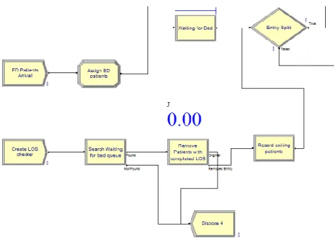
17. Waiting for bed process in ARENA model ... 45
18. Dummy variables created to search and remove patients with completed LOS ... 46
xi
20. Discharge process in ARENA simulation ... 48
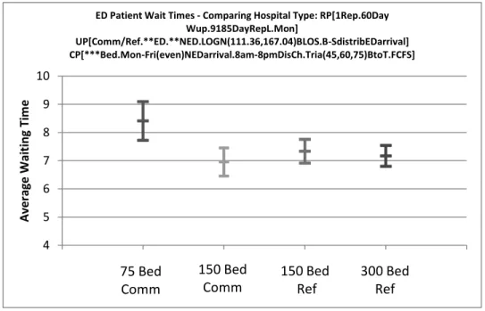
21. ED patient wait time comparing hospital types with baseline values ... 50
22. NonED patient wait time comparing hospital types with baseline values ... 50
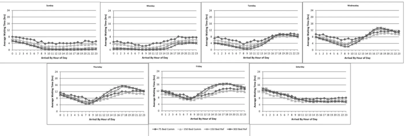
23. ED wait time by day and hour of bed request comparing hospital types using baseline values ... 51
24. NonED wait time by day and hour of bed request comparing hospital types using baseline values ... 51
25. 150 bed community hospital queue length for baseline values from time 0 to 10000 hours ... 52
26. ED patient wait times comparing discharge times for a 75 bed community hospital ... 53
27. NonED patient wait times comparing discharge times for a 75 bed community hospital ... 53
28. ED patient wait time comparing discharge times for a 150 bed community hospital... 54
29. NonED patient wait time comparing discharge times for a 150 bed community hospital ... 55
30. ED patient wait time comparing discharge times for a 150 bed referral hospital ... 56
31. NonED patient wait time comparing discharge times for a 150 bed referral hospital ... 56
32. ED patient wait time comparing discharge times for a 300 bed referral hospital ... 57
33. NonED patient wait time comparing discharge times for a 300 bed referral hospital ... 58
34. ED wait time comparing NonED arrival schedule for a 75 bed community hospital ... 59
35. NonED wait time comparing NonED arrival schedule for a 75 bed community hospital ... 60
36. ED patient wait time comparing NonED arrival schedule for a 150 bed community hospital... 61
37. NonED patient wait time comparing NonED arrival schedule for a 150 bed community hospital... 61
38. ED and NonED patient wait time comparing NonED arrival schedule for a 150 bed community hospital... 62
xii
39. ED patient wait time comparing NonED arrival schedules for a 150 bed
referral hospital ... 62
40. NonED patient wait time comparing NonED arrival schedule for a 150 bed referral hospital ... 63
41. ED patient wait time comparing NonED arrival schedule for a 300 bed referral hospital ... 64
42. NonED patient wait time comparing NonED arrival schedule for a 300 bed referral hospital ... 64
43. ED patient wait time comparing LOS for a 75 bed community hospital ... 65
44. NonED patient wait time comparing LOS for a 75 bed community hospital ... 66
45. ED patient wait time comparing LOS for a 150 bed community hospital ... 67
46. NonED patient wait time comparing LOS for a 150 bed community hospital ... 67
47. ED patient wait time comparing LOS for a 150 bed referral hospital ... 68
48. NonED patient wait time comparing LOS for a 150 bed referral hospital ... 69
49. ED patient wait time comparing LOS for a 300 bed referral hospital ... 70
1
CHAPTER 1
INTRODUCTION
1.1
Motivation
This study was motivated by the knowledge of hospitals being overcrowded more than ever. A decrease in the total number of US hospital beds (hospital closures), nursing shortage, poor economic status of hospital businesses, and an aging US population has all contributed to the crowding occurring in hospitals today. Many hospitals have more patients than they can handle. A congested hospital experiences delays in elective and emergency admissions which gave the foundation to the problem in this study.
1.2
Background
There is not a single answer to the problems that the health care industry faces today. Although technology and medical advances are being made at incredible rates, the process of delivering care is still inefficient where wait delays and cancelations occur regularly. Hospitals have responded by adding resources such as more beds, larger facilities, and increased staff to mitigate the delays but have found this alone is not the answer. But rather, the answer is believed to lie within understanding patient flow as a system and improving ways patients are able to receive timely care (Haraden and Resar, 2004).
The health care industry takes 15% of the United States’ gross domestic product as of 2006 while 45% of the cost is funded publically (Gupta and Denton 2008). Not only do delays have a financial burden on the provider as patients have waiting time thresholds, cause longer turnover time, and increase the number of ambulance diversions, wait times impose an even
2
greater risk of jeopardizing the quality of patient care. Patient waiting causes unnecessary suffering, adverse medical outcomes, further complications of handling delayed patients, added costs and reduced efficiencies. Improving the health care process by finding bottlenecks and system failures will involve understanding the system as a whole as patients flow through the system. Understanding the interactions between patients, clinicians, support services, and
resources will help show how different departments within the hospital interact (Hall et al. 2006). We believe that one method of improving and understanding the causes of waiting time is
through building a discrete event simulation model that simulates the admission and discharge process of patient flow of both ED and elective admissions (NonED).
By studying the admission process, the overcrowding that exists in emergency
departments all over the United States can also be better understood. Overcrowding is considered to be a serious public health problem in 91% of surveyed hospital directors and is forecasted to maintain or get worse due to increased closures of EDs, increased ED volumes, growing number of uninsured, and decreased reimbursement of uncompensated care (Olshaker and Rthlev 2006). Overcrowding in the ED creates delays, cause patients to leave without seeing a physician, decrease patient satisfaction, increase patient pain and suffering, and negatively affects the quality of care provided (Han et al. 2007). The inability to transfer emergency patients to inpatient beds is considered to be the most important factor causing overcrowding in the emergency department (Olshaker and Rathlev 2006). Studying the admission and discharge process of patients will also help benefit overcrowding issues within the emergency department.
1.3
Discrete Event Simulation
As the admission process is a multi-factorial problem involving many different input variables and processes such as ED and NonED admission rates, discharge hours, waiting for bed queue and LOS distributions, a discrete event simulation (DES) software was used. The use of
3
discrete event simulation provides a flexible means to model, analyze, and understand dynamic systems. Computer simulations is considered to be a promising tool which provides a method to study and improve processes without affecting patient care or needing significant monetary investments (Khare et al. 2009).
Discrete event simulation software is also considered as a research technique able to ask what if questions and test different process scenarios while assessing the efficiency of the health care process (June et al. 1999). DES models also provides greater flexibility by being able to use custom parameters and variables compared to the more traditional queuing analytic theory approach. Also, due to the complex nature of the health care industry, DES models have gained popularity to be used to effectively improve the process of health care systems (Duguay and Chetouane 2007). The chosen discrete event simulation software is ARENA version 13.5 created by Rockwell Automation Inc.
1.4
Problem of Description
The hospital admission and discharge process system is complex involving many components and is simplified within this study to better understand the major variables affecting the process. The simplified model will have two types of patients, patients admitted into the hospital through the emergency department (ED) and elective (NonEd) patients. ED patients are those who are admitted to the hospital through the emergency department who are in need of additional emergent/urgent care within the hospital. ED patients are admitted at random and can be admitted any time of the day and has a stochastic element. NonED patients are those who are admitted mostly by appointment with a majority of patients admitted during the day on weekdays and are scheduled ahead of time.
Each patient will enter a bed request queue upon arrival and will wait for an open bed. If a clean bed is available, the first person in the queue will be given a bed, spend time through
4
receiving care, and be discharged once the care is completed. As a patient is discharged, the bed will be cleaned and prepped for the next patient. This simplified process can be seen in Fig X. below.
Figure 1 Simplified admission discharge process
In reality, the admission and discharge process is more complex with different types of beds, many types of patients (intensive care, intermediate care, monitored or unmonitored, surgery) being moved around, with beds even set aside for only specific types of patients (i.e. male, female, children, adult). Even this scenario is a simplified version of reality. However, we are creating a model with the belief that a simplified version will help better understand the real system and provide invaluable information about the process.
Once beds are all occupied, the hospital is at full capacity which create delays in bed availability, and cancelations accrue to create a system that causes hospitals to inefficiently serve their patients. Patients waiting to be admitted through the ED are known as boarding, where patients wait in the ED to be admitted into the hospital. Boarding also increases the chance of overcrowding in the ED as the bed that is used by the patient waiting to be admitted is not able to be used for patients needing emergency care. Elective patients who are scheduled for an
5
appointment or surgery who need to be admitted to the hospital can also be delayed due to full capacity which can also cause cancelations. The figure below displays the simplified admission discharge process at full capacity.
6
CHAPTER 2
LITERATURE REVIEW
A literature review was conducted on the hospital admission system and the use of simulation as a means to understand and decrease waiting time. There is a need to understand the literature within this field as an introduction to the topic but also provide a foundation to this study. A number of databases: PubMED Central (PMC), Pub Med, Web of Science, Academic Search Premier, Engineering Village were searched through the Umass Amherst Library website. Articles focusing on those that predated the past 20 years were not included due to the major changes in the medical practice with the turn of the 21st century. The review was broken into a number of categories; admission scheduling, elective admission, emergency department, and computer simulation in health care processes.
2.1
Admission Scheduling
Helm et al. (2011) simulated a partner hospital through a custom designed c++ program. The group studied the effects of zone based admission control using one year of historical data of arrival rates, length of stay distributions, and transfer probabilities. In the study, expedited patients were identified within the ED as a third class of patients. Patients who are being
admitted through the ED that are able to delay their admission 1-3 days but unable to wait and be admitted as an elective patient due to excessive waiting times are the types of patients which fit the expedited patient category. This study provides a call-in mechanism to serve this third class of patients which allow the reduction of excess load that is placed on the ED during peak congestion periods. Helm et al. (2011) also suggest in their study a Markov decision process model which focuses on using the expedited patient category and elective admission cancelations
7
to create a balance between bed utilization and hospital congestion to provide an optimal admission policy.
Helm et al. (2009) also studied patient flow and admission control and found that hospitals are able to improve hospital occupancy and alleviate congestion by reducing variability through a more flexible system. It was found that many hospitals make decisions independently without considering the downstream effects on workload strain and costs of hospital resources. High variability of elective surgeries due to independent scheduling of each surgeon creates blockages for ED inpatients beds, increases ED waiting times and lowers the quality of health care. Using a patient flow simulation framework of a 160 bed hospital with three main units; surgery, medicine, and ICU beds, they showed that level loaded scheduling with call-in and cancellation thresholds compared to a hospital with the typical front loaded scheduling without daily control thresholds provided a dramatic reduction in the number of cancelations and reduction in variability by 27%. Such improvements could provide healthcare facilities with a means to efficiently staff hospitals to match workload and patient demand with overall
improvement in quality of care and cost savings from reduction of understaffing and overstaffing.
Haraden and Resar (2004) discusses the importance of patient flow in hospitals as a major area to study for understanding and improving patient wait and cancelations. Hospitals have responded by adding more resources through more beds, larger facilities, and increased staff numbers but have seen that just increasing resources does not solve the common occurrences of waiting. Interventions that smooth the flow of elective surgery, reducing waits for inpatient admission through the ED is critical in that understanding variation is the first step in providing timely flow of patients.
Lowery (1996) explains that when creating a hospital admission scheduling system through simulation, the simulation model should be able to be easily applied to multiple hospitals,
8
be valid, representing an actual system, and be able to show improvements in variability. Some of the input variables that are highlighted include number of beds, average standard deviation of LOS, arrival rates of emergency patients by day of week, and distribution of elective admits. Using a graphical approach is the most common method of validating a model and explained how understanding the admission process would prove to be invaluable to explaining how the system behaves.
White et al. (2011) conducted a study on the interactions between patient appointment policies and capacity allocation policies and their effects on performance measures in an outpatient healthcare clinic. They found that scheduling lower-variance, shorter appointments earlier would maintain physician utilization and clinic duration but lower overall patient waiting. From the study they also saw that the number of exam rooms displayed a bottleneck behavior where there would be no effect on physician utilization beyond a certain point and cause critical problems when too low.
Boston Medical Center in 2004 showed that elective surgery scheduling had a big impact on hospital systems and was a larger source of bottlenecks on patient throughput than emergencies. By also incorporating non-block scheduling of a pavilion at Boston Medical Center, dramatic results were seen with 334 elective surgeries that were canceled or delayed before the change dropped down to 3 delays/cancelations. Actively addressing patient flow problems through studying the issues and developing methods to modify the process is seen as a critical step in creating a more efficient health care delivery system.
The Chartis Group (2007) introduced the potential benefits of optimizing patient throughput not only on improved operating performance but also on the return on assets and use of capital. The group noted that some hospitals have had 5-12% increase in available capacity by just improving admission throughput which also improves the number of discharges per available
9
bed, increasing overall net revenue. In order for a hospital to optimize patient throughput, there has to be an organizational commitment where each part of the process must be aligned as a coherent system.
Kloehn (2004) in an executive summary tries to address how problems with patient throughput causes a wide array of unsolved issues in overcapacity, diversions, excessive wait times, bed placement control, and discharge process. A facility over 85% occupied is considered to have a high chance of throughput issues and delays in the ED. Throughput is also to have an impact in how patients are admitted and cause unnecessary delays and excessive wait times.
2.2
Elective Admission
Bowers and Mould (2002) conducted a study on reducing waiting time through "deferrable elective patients" to maximize utilization and still ensuring quality of care for orthopaedic patients in the UK. "Deferrable elective patients" are elective patients given the opportunity to receive earlier care with the possibility of postponement based on the event that the demand of care needed for that day is high. Using this policy would allow for patients to be seen earlier having an impact on waiting time but with the cost of 19% probability of treatment being deferred.
Gupta and Denton (2008) summarized key issues in the health care field using different kinds of models to help represent a scheduling system. There was concern that existing
manufacturing, transportation and logistics models are not able to easily fit into the health care field due to the nature of the health care industry. There are many issues that must be addressed such as patient and provider preferences, stochastic and dynamic nature of multi-priority demand, technology changes, and soft capacities to name just a few. The paper also describes the
challenges and future opportunities to implement novel industrial engineering and operation research techniques to hospital appointment scheduling systems.
10
May et al. (2011) reviews the problem of surgical scheduling by surveying past work and suggesting potential future research on capacity planning, process reengineering, surgical services portfolio, procedure duration estimation, schedule construction, and schedule execution,
monitoring and control. Surgical scheduling was considered to deviate significantly from even a detailed plan through the course of a surgical day due to the stochastic elements of arrivals, cancelations, and duration of the surgical procedures. However, the study concluded with the idea that a better guide will allow operational management to use their resources more effectively and efficiently with the economic and project management aspect of surgical scheduling having the greatest potential for relevant research.
Min and Yih (2009) studied patient priority within the elective surgery scheduling problem. Using a stochastic dynamic programming model, patients with the highest priorities were selected to be scheduled for surgery when capacity became available. The study showed that using patient priority had significant impacts on surgery schedules.
Bekker and Koeleman (2011) assessed a study on scheduling elective admissions that minimized the target and offered load of patients in order to maintain more consistent bed occupancy levels. Target load levels were determined based on the capacity in relation to the variability in offered load as well as incorporating weekly patterns of bed availability. Smoother admission best stabilizes bed occupancy levels. The more even distribution of elective
admissions throughout the week provided the most stable time performances by decreasing variability in bed demand and the probability of refusals. The article also found that patients with longer LOS scheduled on Fridays provided a more optimal schedule while higher admissions on Mondays with shorter LOS also were found to be advantageous. The model in this study however does not capture the discharge process.
11
Gallivan et al. (2002) conducted a study looking at inpatient admissions of a cardiac surgery department and hospital capacity using a mathematical model. The LOS although averaged less than 48 hours, had considerable overall variability with a lengthy tail which was found to have considerable impact on capacity requirements. A reserve capacity was required in order to avoid high rates of cancellations. Caution was advised when considering booked admission systems when there is a high degree of variability in length of stay due to the result of possible frequent operational difficulties for hospitals with limited reserve capacity.
2.3
Emergency Department
Forster et al. (2003) studied the effects of hospital occupancy on emergency department length of stays and patient disposition. They conducted an observational study of a 500 bed acute care teaching hospital which showed that increased hospital occupancy seemed to be a major indicator of increased ED LOS for admitted patients. A threshold of 90% bed occupancy appeared to indicate extensive increase in ED length of stay which is believed to be a an important determinant of ED overcrowding. Also, although there is little data verifying the claim, they suggested increasing hospital bed availability might contribute to less ED overcrowding especially when at the 90% bed occupancy threshold.
Han et al. (2007) assessed a study on the effects of expanding the emergency department and its effects on overcrowding. An increase in ED bed capacity had little effects on ambulance diversion, and increased the length of stay for admitted patients due to other bottlenecks within the hospital network.
Olshaker and Rathlev (2006) explored how emergency department overcrowding and ambulance diversion impacts boarding times of patients waiting to be admitted into the hospital. The inability to admit ED patients have been highlighted by the Joint Commission on
12
as the leading factor contributing to ED overcrowding. Olshaker and Rathlev (2006) also covers the causes of overcrowding through the development and changes within the health care industry as there is an increase in ED visits due to a number of ED closures, a greater percentage of patients not having health insurance, and a number of laws and programs effecting increased volumes.
Asplin et al. (2003), provide a conceptual model of the emergency department, described as an acute care system, a delivery system providing unscheduled care. We are most interested in the output component and the discussion of boarding, the inability to move admitted ED patients to an inpatient bed which is the most frequent reason for ED crowding and a reason for the ED’s inability to take on new patients. Some factors found to cause inpatient boarding in the ED is the lack of “physical inpatient beds, inadequate or inflexible staffing, isolation precautions, delays in cleaning room after patient discharge, over reliance on ICU or telemetry beds, inefficient
diagnostic and ancillary services on inpatient units, and delays in discharge of hospitalized patients to post-acute care facilities.”
Derlet et al. (2000) published a paper on the complexity of emergency departments and its interwoven issues as reasons for overcrowding and its effects on “patient risk, prolonged pain and suffering of patients, long patient waits, patient dissatisfaction, ambulance diversions, decreased physician productivity, increased frustration among medical staff, and violence." One reason for overcrowding in the study was due to the lack of beds for patients being admitted to the hospital, where patients in the ED must wait, known as boarding until a bed is freed which seem to be common in all ED’s. The paper goes on to discuss other issues as well as a more detailed explanation of the effects of overcrowding and overall decrease in quality of healthcare.
Khare et al. (2008) studied the influence of emergency department crowding by
13
study showed that by improving the rate at which admitted patients left the ED decreased the overall ED length of stay, while increasing the number of beds did not. Admitted patient departure from the ED proves to be a major factor and a possible bottleneck in ED crowding and is of important value to study.
Liu et al. (2012) conducted a study through survey on the effects of reducing crowding in the emergency department through crowding initiatives like vertical patient flow, a method of evaluating and managing patients without using an ED room. Further study was suggested in examining the effects of such crowding initiatives in patient outcomes (safety, LOS, satisfaction) as there is yet a widespread support system in place to create enough momentum to see
improvements in ED crowding.
2.4
Computer simulation in health care processes
The use of simulation is growing and is seen as a powerful tool within the health care industry being able to model a wide range of topic areas and answer a variety of research questions as explained in the systematic review regarding computer simulation in health care done by Fone et al. (2003). The review also discusses how computer modeling should provide valuable evidence in how to deal with stochastic elements within the industry. However, it is still yet to be seen the effects and true value of modeling such processes due to the lack of model implementation on real systems.
Duguay and Chetouane (2007) modeled the emergency department using discrete event simulation and found DES to be an effective tool due to the complexity of healthcare systems. They suggested the combination of total quality management and continuous quality
improvement techniques to specially be useful in combination with DES. The group studied a regional hospital to improve the current process through data collection and the use of control variables (physicians, nurses, and examination rooms). Analysis of waiting times and best
14
staffing scenarios was conducted by adding and reducing staff and exam rooms within budget limitations.
Kumar and Mo (2010) provide three different methods of bed prediction models, one of which was simulated through ARENA 10.0 to model bed occupancy levels for 3 different wards for three different types of patients. Data was collected from a hospital for values on the daily number of admissions, average length of stay over one year, and average number of beds for each patient type. The simulation showed to be a useful tool in predicting bed occupancy levels for coming weeks and actual values fell within the 95% confidence interval of the model.
Jacobson et al. (2006) reviewed journal articles using discrete event simulation on health care systems and showed the benefits of using optimization and simulation tools to give decision makers optimal system configurations. Using discrete-event simulation to analyze health care systems have become more accepted by healthcare decision makers. A benefit of using discrete-event simulation is the ability to incorporate multiple performance measures associated with health care systems to help understand the relationships that exist between various inputs.
Jun et al. (1999) also reviewed the literature involving discrete event simulation and found that distributing patient demand improved patient flow by decreasing waiting times in outpatient clinics. The survey also shows that there has been many studies on patient flow that use discrete event simulation but found a void in integrated multi-facility systems.
Sargent (2011) discusses verifying and validating simulation models through different approaches, graphical paradigms, and various techniques. The author mentions that there is yet to be a set of specific tests that easily applies to the validity of a model giving every new simulation project unique challenges.
15
Eddy et al. (2012) conclude the importance of creating a model that is transparent, showing how the model is built and valid in reproducing reality to become successful within the health care industry. Face, internal, cross, external, and predictive validity are all a means to validate a model with the latter two being the strongest forms. Validation of a model is also suggested with 4 criteria in mind: rigor of the process, quantity and quality of sources used,
model's ability to simulate sources with detail, and how closely results match observed outcomes.
There are also many studies of simulation that have been applied to the emergency department such as studies done by Miller et al. (2003), Samaha et al. (2003), and Blasak et al.
(2003).
16
CHAPTER 3
METHODOLOGY
3.1
Baseline parameters
The baseline parameters can be defined as the input parameters of the simulation model known to be standard within this study. The set of baseline parameters also acts as a guideline for future studies and researchers by providing the standard needed for reproducing the model. Many instances within the study compare a single parameter change to the baseline values.
3.1.1 Replication Parameters
Replication parameters are the values that provide information on the replication within the simulation software, found under Run Setup. Replication values include the number of replications, replication length, warm up period, replication start day, as well as time units. The replication parameters remained the same for every simulation in this study, and were not altered.
17
3.1.1.1 Number of Replications
The simulation model within this study initially exists in an empty and idle state, where there are no patients and no beds utilized in the hospital. As the simulation begins to run, patients enter the hospital and start filling beds without waiting in a queue due to the capacity of beds being underutilized. In a real life setting, a hospital is never empty, and therefore, a steady state simulation was necessary for this study. Understanding the capacities at any given time should not be affected by the initial idle state of the model. A steady state simulation model will help to understand the hospital's long-run performance measures and give insight into the waiting times of patients.
In a steady state simulation, you can estimate a long run performance measure with a specified confidence interval by increasing the number of replications, or by increasing the run length of the simulation (Banks et al. 2005). The simpler method would be to make independent and identically distributed replications with a warm up period allowing to gather and analyze data of a process in a steady state. However, because a part of the analysis involved in this study required manual manipulation of exported data, having multiple replications made it difficult to capture the data from each replication. Due to this reason, the second method of creating a steady state simulation using a single replication with a long run length was found to be more
advantageous. In every simulation run in this study, there is always 1 replication.
3.1.1.2 Warm Up Period
One method to help a simulation reach a steady state is with the use of a warm up period until the initial conditions bias on the data have subsided. After the point the warm up period is set for, the data would be reset and statistical information would be gathered from that point on. In our model, this would represent the point where we believed that the hospital could reflect the utilization on any given day. Kelton et al. 2007 explained in their simulation textbook that
18
determining how long a warm up period is difficult and advised to make key output plots and eyeball where they stabilized.
The two different output plots used in order to determine the warm up period are bed utilization and the waiting for a bed queue. For these sets of plots, the same model was used with a shortened simulation length in order to plot multiple replications. Only the initial period of the simulation is important until there is a period in which the simulation enters into a state of steady state. The following two graphs show plots from 10 different simulation replications displayed by the ARENA output analyzer over a period of 2000 hours or 83.33 days.
19
Figure 5 Queue length of a 150 bed community hospital with 10 replications
From the two graphs, first of bed utilization and the second of the queue length of patients waiting for a bed, we are able to estimate a warm up period that is believed to be
satisfactory. In the graph of bed utilization, we can see that the percentage of beds being utilized reaches 100% quite rapidly and in all replications within 500 hours or 20.83 days. The queue length of the 10 different replications has many peaks which is believed to be random and reaches a steady state by half way point in the graph, 1000 hours or 41.67 days. To be conservative, our warm up period was extended to 60 days in all the simulation runs within this study to create a system where the hospital is in a steady state.
3.1.1.3 Replication Length
A single replication simulation run requires a longer replication length in order to find a performance measure with a desirable confidence interval. Under a single replication, the data
20
becomes dependant when computing the standard error of a mean. To solve this problem, batch means could be used by splitting the single replication into a number of batches, with means considered to be independent of each other (Banks et al. 2005). The batch means are in essence a method to provide measures that are comparable to the means of a simulation with multiple replications. ARENA automatically batches single replications in sizes which attempt to make the data uncorrelated. ARENA attempts to compute a 95% confidence interval through batch means automatically and creates half widths for the output statistics. ARENA does not use data from the warm up period when calculating batch means and will not report a half width if the internal checks done through the program signal that the batch means collected were correlated (Kelton et al. 2007).
The method that ARENA uses to batch data is by forming 20 batches when enough data is collected. A time persistent statistic will form a batch with the average over 0.25 base time units. As the simulation is continuingly collecting data, once 20 batches are made, ARENA continues to count batches with the same batch sizes until 40 batches exist. At this point, the 40 batches are reformed by combining the means of batch 1 and 2, 3 and 4, and so on until 20 batches exist. The 20 batches have twice as many points compared to the original 20 batches, and the simulation program continues to create the 21st batch with the new batch size. Once 40 batches are made, they are again formed into 20 newer batches with again double the points of data. This method is used based on the reason that it is not more advantageous to continue to collect data and increase the number of batches which are more likely to produce correlated batch means if the batches are originally too small. (Kelton et al. I2007)
Original models that were used in the early stages of this study used 5 replications with a 5 year replication length. As we transitioned into a 1 replication model, we converted all the replications to a single simulation run of 25 years. A 25 year simulation length allowed the data collected to have batches that were believed to be unbiased, independent and identically
21
distributed due to the conservative lengthening of the simulation. ARENA also producing values of half widths with a 95% confidence interval for each of the statistical outputs also confirmed the chosen replication length was sufficient.
The replication length in each of the simulations conducted in this study was set to 9185 days, which is 25 years plus 60 days of warm up. This allows the replication length to fully incorporate 25 years of data.
3.1.1.4 Replication Start Date and Base Time Units
In order to have a standard between replications there was a need to pick a replication start date since the arrival rates of patients depended on the day of the week. January 2, 2012 was chosen as the start date, but more importantly, the simulation starting day of the week was
Monday. The base time unit in this study that fit with all the different arrival rates and discharge times is hours.
3.1.2 Uncontrollable Parameters
Uncontrollable parameters were the values in the model that were believed to be fixed and uncontrollable in the hospitals current state. Within a given situation, the UP, uncontrollable parameters would in most cases be set based on a number circumstances including the area a hospital is located, the types of patients served, type of facilities available, and access to certain technologies. Some of the uncontrollable parameters were the type of hospital (community versus referral), percentage of ED and NonED patients, patient length of stay, and the arrival rate of ED patients.
Every simulation was categorized using a shorthanded description of the model using brackets and periods to separate categories within the parameters. For uncontrollable parameters
22
the categories were listed in order based on the type of hospital, then the percentage of ED and NonED patients, length of stay, and the ED admission arrival rate.
The following is an example of this short hand representation describing a hospital as a community hospital, with 70% ED and 30% NonED patients, a length of stay with a lognormal distribution with the mean being 111.36 hours with a standard deviation of 167.04 hours, while using the Baystate distribution of ED patients.
UP[Comm.70ED.30NED.LOGN(111.36,167.04)BLOS.B-SdistribEDarrival]
3.1.2.1 Type of Hospital
Creating two types of hospitals, a tertiary referral hospital and a local community hospital would allow this study to be applicable to a larger population of hospitals in the country. In our study, a tertiary referral hospital was categorized as a hospital able to accommodate referrals from lower levels of care, that can treat more complex clinical conditions through specialized
personnel, and advanced technologies (Hensher et al. 2006). Community hospitals were considered to be smaller in size, treating a larger portion of their patients admitted through the emergency department. It would be nearly impossible to fit every health care facility or system in specific categories, but there were major differences in the size and patient type distribution that was addressed. This study allows a general comparison of different size hospitals while also considering the difference in their patient makeup. Often times, a community hospital would be located in a rural area while a referral hospital is in an urban setting.
A study done by HCUP, Healthcare Cost and Utilization Project categorized the number of beds between small, medium, and large size hospitals between regions, and location. Using the values found in the HCUP's data, 150 beds was chosen to represent the size of a large community hospital and a small/medium referral hospital. In order to compare community and
23
referral hospitals it was important the two different hospital types shared the same number of beds. A smaller community hospital with 75 beds was also considered while a 300 bed referral hospital was created as well. The representation of community hospitals having 75 and 150 beds while referral hospitals with 150 and 300 beds allowed a symmetric increase in size while also being able to consider the different type of patients that were admitted more effectively.
3.1.2.2 Hospital Patient Make Up
Once the size of the different hospitals was determined, the patient make up of each hospital was considered. In this study, there are two different types of patients admitted into the
hospital, ED and NonED patients. Hospitals in Massachusetts were examined in order to create the standard patient spread for each type of hospital by categorizing hospitals to be either community or referral. Each hospital’s percent of admissions from the ED was factored into the
baseline values. An assumption was made that the remainder of patients that were admitted would be considered as NonED patients.
Table 1 Mass hospital percentage of admission in 2010
Source: Inpatient hospital discharge database, 2011, Division Health Care Finance and Policy Efficiency of ED utilization in Massachusetts 2012, Division Health Care Finance Policy
Mass Hospitals FY10
Local Hospitals ED volume ED Inpt Admits ED Obs Admit Total Inpt Discharges % ED Inpt Admits Discharges/day
Baystate Franklin 29,203 2,722 925 4,292 63.4% 11.8
Baystate MaryLane 15,684 1,127 603 1,493 75.5% 4.1
Baystate Medical 112,447 19,833 7,612 37,988 52.2% 104.1
Berkshire Medical - Birkshire 56,514 8,152 2,153 10,775 75.7% 29.5
Cooley 36,735 6,416 895 9,161 70.0% 25.1 Harrington 35,707 2,954 1,555 4,056 72.8% 11.1 Holyoke 42,533 4,858 2,043 6,691 72.6% 18.3 Mercy 76,582 7,177 2,178 12,131 59.2% 33.2 Noble 27,567 2,485 2 3,475 71.5% 9.5 Total Mass 3,093,778 468,635 115,455 851,154 55.1% 2331.9
Referral Hospitals ED volume ED Inpt Admits ED Obs Admit Total Inpt Discharges % ED Inpt Admits Discharges/day
Beth Israel 55,046 19,431 6,807 41,595 46.7% 114.0
Boston Medical Center 127,643 18,382 6,249 30,251 60.8% 82.9
Brigham & Womens 56,437 13,427 6,361 51,754 25.9% 141.8
Childrens - Boston 47,560 NA NA 18,147 49.7
Mass General 89,587 21,826 3,180 50,337 43.4% 137.9
Tufts 41,437 8,279 906 21,075 39.3% 57.7
24
The average for % ED Inpatient Admits for the local community hospitals resulted in 70.1% which was rounded to 70%. 70% of patients admitted through the emergency department would result in 30% of patients admitted as NonED patients. The same process was taken for the referral hospitals which resulted in ED patients averaging 45.7% which was rounded down to 45% and of the patients admitted into a referral hospital, 55% would be NonED patients. The following table gives a breakdown of the baseline values used for the different types of hospitals used in this study. The percent spread of each type of hospital does not change throughout this study.
% Admissions for ED/Non ED
% from ED % Non ED / Elective
Admissions
Community Hospitals 70% 30%
Tertiary Hospitals 45% 55%
Table 2 Baseline percent admission for community and referral hospitals
3.1.2.3 Length of Stay (LOS)
The method of determining a patients length of stay was using existing data from
Baystate Medical Center, finding a distribution, and applying national numbers. The point of this study is to provide a general relationship between different types of hospitals and the admission of patients on a scale that could represent a majority of existing hospitals. Due to our objectives, it was important when possible not to use data specific to any given hospital.
Ozen et al. 2012 collected data from Baystate Medical Center in Springfield
25
discharged for a six month period. Time stamps were taken for four different types of patients, ED admits that had no surgery, ED admits who needed surgery, NonED admits needing surgery, and NonED admits non needing surgery. The LOS for each type of patient was heavily skewed right with the tail reaching times much further away from the majority of the data points. The following is a graph from their research showing the length of stays for NonED patients not needing surgery.
Figure 6 Length of stay distribution of NonED patients not needing surgery Asli 2012
The distributions with heavy right skews were best choices: we looked at johnson, lognormal, and Glog distributions. After analyzing the different distributions that would fit a skewed LOS, it was determined that using a lognormal distribution would best allow the input of national data on length of stay requiring only two parameters, the mean and standard deviation. Again, the use of national data allows this study to be more viable for a broader range of hospital systems.
26
National averages on the length of stay of patients were obtained from the 2010 HCUP Nationwide Inpatient Sample (NIS) , a database of hospital inpatient stays, the largest inpatient care database publically available in the United States.
NIS's length of stay is calculated by subtracting the date of admission from the date of discharge. Same day stays are therefore counted with a length of stay of 0. The average length of stay for inpatients from the 2010 HCUP NIS data came out to 4.64 days with a standard deviation of 6.96 days. Since the simulation's base time units is in hours, we converted the values resulting in an average LOS of 111.36 hours with a standard deviation of 167.04 hours.
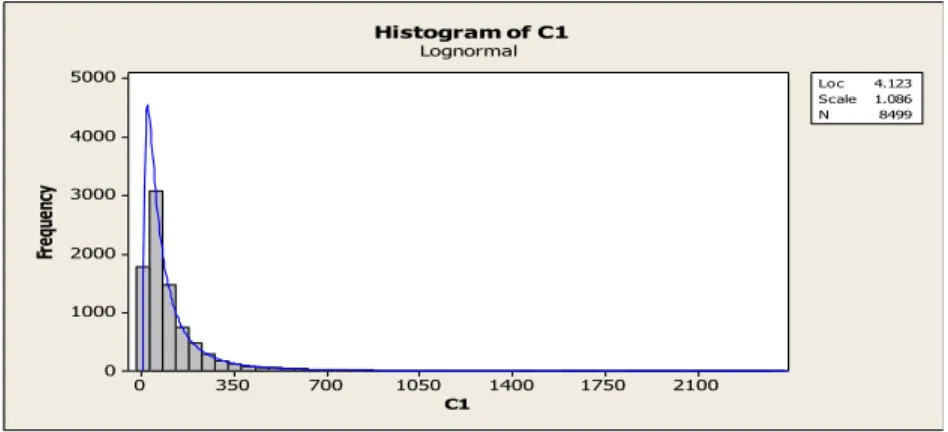
The length of stay baseline value used in our simulation model was a lognormal distribution having a mean of 111.36 and a standard deviation of 167.04 hours. In order to confirm in our ARENA software, a one year simulation run exporting the LOS values was conducted using the input lognormal(111.36, 167.04) for the LOS value. The following graphs shows the output values as the bar graph compared to the lognormal distribution shown as the blue line.
Figure 7 LOS lognormal distribution compared to ARENA LOS exported data
ARENA exported data represented as bar graph, lognormal distribution represented with blue line
2100 1750 1400 1050 700 350 0 5000 4000 3000 2000 1000 0 C1 Fr eq ue nc y Loc 4.123 Scale 1.086 N 8499 Histogram of C1 Lognormal
27
The location and scale parameters of the lognormal are the mean and standard deviation of the natural logarithm where the log of the lognormal distribution would be normally
distributed. The location and scale parameter can be found using the E[X] as the expected value of the distribution and the Var[X] being the variance (standard deviation2).
Figure 8 Equations of lognormal location and scale parameters
Calculations finding the location and scale parameters
Mean = 111.36 SD = 167.04 Mean^2 = 12401.0496 SD^2 = Var = 27902.3616
μ = ln(111.36) - (1/2) * ln(1+ (27902.3616/12401.0496)) = 4.1234 σ^2 = ln(1+ (27902.3616/12401.0496)) = 1.1787m =
σ =
1
.
1787
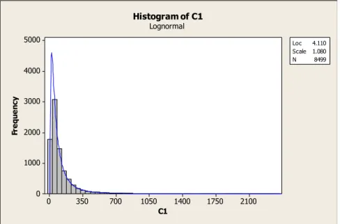
= 1.08567However, in ARENA we are able to input the mean and standard deviation of the lognormal directly. The one year simulation run had an average of 108.04 hours and a standard deviation of 147.468. By also best fitting the exported values of the LOS to a distribution, we obtained the following lognormal, which confirmed that the input parameters of the LOS
distribution was indeed a skewed right lognormal distribution that would converge to the baseline values of 111.36 hours with a standard deviation of 167.04 hours if ran for a longer period of time. LOS in our model represented the time the patient spent in the system from the moment they entered until the time they are ready to be discharged.
28
Figure 9 ARENA LOS exported values best fitted to a lognormal distribution
3.1.2.4 Weekly Arrival Rate
In order to create a crowded hospital system considering the given length of stay alongside the number of beds available, Little's Law was used to determine the weekly arrival rate of patients. Little's Law states that under steady state conditions, the number of beds in the system will equal the average rate of arrivals times the average time spent in the system.
Little's Law
L = # of Beds in the system
λ = Average number of patients arriving per unit time W = Average time spent in the system, length of stay
L = λW
Example of using Little's Law in our study
The following shows the arrival rate of a community hospital with 150 beds. λ is the average arrival rate of both ED and NonED patients into the system.
2100 1750 1400 1050 700 350 0 5000 4000 3000 2000 1000 0 C1 Fr e q u e n cy Loc 4.110 Scale 1.080 N 8499 Histogram of C1 Lognormal
29
L = 150 Beds
W = LOS = 4.64 days L = λ *W
λ = L / W = 150/4.64 = 32.33 patients per day
Due to the different arrival rate schedules, the arrival rate was converted to a weekly arrival rate by taking λ * 7.
Average arrival rate per week = λ * 7 = 32.33 patients per day * 7 = 226.29 patients per week
# of Beds in the Hospital Average daily arrival rate of patients
Average weekly arrival rate of patients
75 16.16 113.15
150 32.33 226.29
300 64.66 452.59
Table 3 Arrival rate chart based on hospital size
The number of patients arriving per week whether a community or referral hospital does not change based on the type of hospital when considering a 150 bed system. Both 150 Bed hospital systems, community and referral will see an average weekly arrival of 226.29 patients.
3.1.2.5 ED Patient Arrival Distribution
The hourly distribution of ED patients were determined to be an uncontrollable parameter because hospitals cannot restrict or determine when patients are able to receive care. Emergency departments are open 24/7 and patients arrive throughout the day Monday through Sunday unscheduled and also random. Admission arrival rates into the hospital from the emergency department have been collected from Baystate Medical in Springfield, Massachusetts by hour of
30
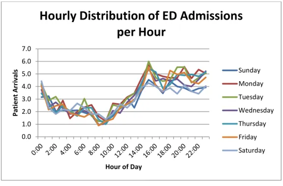
the day for each day of the week over a 6 month period. The daily arrival of patients being admitted from the ED followed a consistent trend shown below.
Figure 10 Average patient arrival for ED patients each day of the week at Baystate Medical Center
The arrival process of patient admission for different departments generally follows a Poisson process (Bekker and Koeleman 2011). The arrival rate for ED patients are often considered to follow a Poisson distribution. The data also would indicate that the inter-arrival rate for ED patients by hour of the day follows an exponential distribution, giving the arrival rate of hospital admissions by hour of the day from the ED a Poisson distribution. The actual
percentiles of ED arrivals per hour is compared to the percentiles of a Poisson distribution using the actual mean indicate that the arrival rate of ED patients is Poisson distributed.
0.0 1.0 2.0 3.0 4.0 5.0 6.0 7.0 Pati e n t A rr iv al s Hour of Day
Hourly Distribution of ED Admissions
per Hour
Sunday Monday Tuesday Wednesday Thursday Friday Saturday31
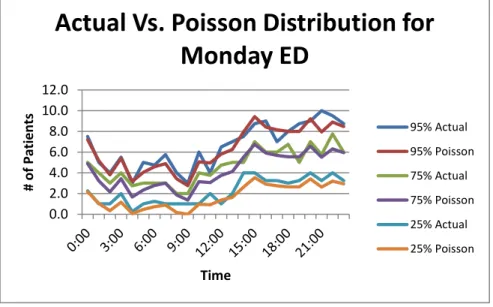
Figure 11 ED admission comparing actual distribution to a Poisson distribution on Mondays at Baystate Medical Springfield Massachusetts
In order to create a simpler model for this study, there was an assumption that each day of the week could be represented by a single distribution of ED arrivals by taking the average of the entire week. From the average, a single distribution of the percentage of patients arriving per hour for ED patients was created shown in the following graph. This graph shows based on the daily arrival rate of ED patients admitted into the hospital, the number of patients by percentage admitted each hour that was used in this study. For example, 5% of the daily ED admits will arrive at midnight. We also see from this distribution that there is a larger number of ED patients admitted between 3pm - 12am. The ED hourly admission distribution was used as the baseline values for the distribution of ED patient arrivals on average throughout the day.
0.0 2.0 4.0 6.0 8.0 10.0 12.0 # o f Pati e n ts Time
Actual Vs. Poisson Distribution for
Monday ED
95% Actual 95% Poisson 75% Actual 75% Poisson 25% Actual 25% Poisson32
Figure 12 Average ED admission by percent of the daily arrival rate per hour
Since the arrival rate of ED patients into the hospital follows a Poisson distribution, the input data into the simulation was conducted as a stochastic component of the model. The baseline values depended on the total weekly volume of patients admitted through the ED but follow the same hourly distribution each day. In our simulation model, both the total admissions as well as the arrival rate following a Poisson distribution was checked. The daily arrival rate of patients was found by taking the weekly arrival rate and using the percentage of ED patients based on the type of hospital and dividing by the number of days that ED patients could be admitted per week.
Example of Finding the Daily Arrival Rate of ED patients for a 150 Bed Community/Referral Hospital
Average weekly arrival rate of patients for a 150 bed hospital found using Little's Law = 226.29 patients 0.0% 1.0% 2.0% 3.0% 4.0% 5.0% 6.0% 7.0% 8.0% 0:00 2:00 4:00 6:00 8:00 10:00 12:00 14:00 16:00 18:00 20:00 22:00 Per ce n t A d m issi o n b y Hou r Time of Day
33
% of patients admitted from the ED in a community hospital = 70%
Average weekly arrival of ED patients in a 150 bed community hospital = 226.29 * 70% = 158.405 patients
Average daily arrival of ED patients in a 150 Bed community hospital = 158.405/7 = 22.629 Average weekly arrival of ED patients in a 150 bed referral hospital = 226.29 * 45% = 101.832
patients
Average daily arrival of ED patients in a 150 bed referral hospital = 101.832/7 = 14.547 patients
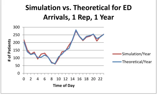
Using the daily arrival rate of ED patients, the hourly arrival rate percentage was multiplied to the average daily arrival rate to find the hourly admission rate of ED patients. The total number of patients arriving in the simulation by hour was compared to the theoretical estimate. From the data we can conclude that the schedule used in the simulation is accurate by the total number of ED patients admitted into the hospital by hour of day.
Figure 13 Comparison of the number of ED patients being admitted in a 1 year simulation run compared to the theoretical value
0 50 100 150 200 250 300 0 2 4 6 8 10 12 14 16 18 20 22 # o f Pati e n ts Time of Day
Simulation vs. Theoretical for ED
Arrivals, 1 Rep, 1 Year
Simulation/Year Theoretical/Year
34
To verify that the input schedule in the simulation for the ED admission rate is Poisson distributed, the number patients arriving for every hour of the day was found in a 1 year
simulation run. The number of patients arriving for each hour was counted and compared to the likeliness of that event based on the Poisson distribution. Six different hours of the day were checked where two of them can be found in the following table. Over a year period, the results show that the simulation is indeed showing an ED arrival rate that is Poisson distributed.
# Patients arriving within the hour
% of event based on Poisson distribution
# of times event occurred in simulation
% the event occurred in the simulation 12am - 1am 0 0.565 207 0.567 1 0.322 110 0.301 2 0.092 38 0.104 3 0.017 8 0.022 4 0.002 2 0.005 12pm - 1pm 0 0.663 249 0.682 1 0.273 91 0.249 2 0.056 22 0.060 3 0.008 2 0.005 4 0.001 1 0.003
Table 4 Two hours with percentages of events occurring with a Poisson distribution compared to actual events during a 1 year simulation run
In this study, there were four different ED arrival rates, all being Poisson distributed, with an hourly distribution based on the daily arrival rate found using Little's Law and the type of hospital being studied. The number of patients being admitted while following the ED distribution is random as it is in hospitals throughout this country. Within the short hand representation describing the values used within a particular simulation run, B-SdstribEDarrival stands for the Bay State ED arrival distribution used to find the percentage of patients arriving each hour of the day.
35
3.1.3 Controllable Parameters (CP)
Controllable parameters are the values that were considered to be controllable within a hospital's management. Such parameters involve values regarding the number of beds, NonED admission rates, allowable discharge hours, the bed turn over time, and patient priority.
The shorthanded description of the simulation model's values for the controllable
parameters are listed in order by the number of beds, NonED admission days, the hours available for patient discharge, the length of time for the bed turn over time, and patient priority.
CP[150Bed.Mon-Fri(even)NEDarrival.8am-8pmDisCh.Tria(45,60,75)BtoT.FCFS]
would represent a model that has 150 beds, allows NonEd patients to arrive Monday through Friday, 8am-8pm available patient discharge hours, a triangular distribution of min, mean, max values of 45, 60, and 75 minutes of time for a bed to be cleaned, and a first come first serve (FCFS) patient priority system.
3.1.3.1 Number of Beds
The number of beds in the simulation is considered to be controllable because hospitals are able to increase or decrease the number of beds which exist. Changing the number of beds may be restricted to the space available as well as financial constraints, however, we felt the number of beds within a hospital in general, is flexible.
The baseline values within this study for the number of beds is covered in section 3.1.3.1 Type of Hospital. There are 3 different sizes of hospitals with different number of beds.
Community hospitals will have 75 beds and 150 beds while referral hospitals will be studied with bed sizes of 150 and 300 beds.
36
3.1.3.2 NonED Admission Rates
NonED patients are admitted into the hospital outside of the emergency department. The admission is considered to be controllable due to the hospital's ability to cancel, delay, and schedule in advanced when the patients are admitted. In this study, the baseline values for NonED admission rates was a Monday through Friday schedule with a uniform distribution over ten hours from 8am-6pm. A baseline of 5 days of NonED allowable admission days is used due to the data from Baystate Medical showing the majority of NonED admits being admitted on weekdays. Weekend admissions were not included in this study.
Like the method used to find the daily arrival rates for ED patients, the percentage of NonED of the weekly arrival rate was multiplied then used to find the daily arrival rate based on the number of allowable days for NonED admissions. A Mon-Fri NonED admission schedules has 5 allowable admission days. The daily arrival rate for 5 NonED arrival days equals the weekly arrival of NonED patients divided by 5.
Example of Finding the Daily Arrival Rate of NonED patients for a 150 Bed Community/Referral Hospital
Average weekly arrival rate of patients for a 150 bed hospital found using Little's Law = 226.29 patients
% of NonED patients admitted in a community hospital = 30% % of NonED patients admitted in a referral hospital = 55%
Average weekly arrival of NonED patients in a 150 bed community hospital = 226.29 * 30% = 67.887 patients
Average daily arrival of NonED patients in a 150 Bed community hospital = 67.887/5 = 13.577
Average weekly arrival ofNon ED patients in a 150 bed referral hospital = 226.29 * 55% = 124.46 patients