THE SHOOTING METHOD FOR SOLVING SECOND ORDER FUZZY TWO-POINT BOUNDARY VALUE PROBLEMS

(1)

ISSN: 1311-1728 (printed version); ISSN: 1314-8060 (on-line version)

doi:_{http://dx.doi.org/10.12732/ijam.v32i4.9}

Basem S. Attili University of Sharjah

College of Sciences - Department of Mathematics Sharjah - P. O. Box 27272

UNITED ARAB EMIRATES

Abstract: We consider the fuzzy two-point boundary value problem (FBVP) subject to some fuzzy boundary conditions on an interval [a, b]. Numerically, we start by transforming the two-point boundary value problem into a system of fuzzy initial value problems (FIVP). To solve the resulting system, we use an improveds−stage Runge-Kutta Nystrom 4th order method adopted to handle fuzzy problems. Numerical results will be presented to give the numerical details and to show the efficiency of the method.

AMS Subject Classification: 65H10

Key Words: fuzzy two-point BVP’s, fuzzy Runge-Kutta method, fuzzy dif-ferential equations, shooting method

1. Introduction

Many problems in applied sciences and engineering are modeled as fuzzy differ-ential equations (FDE) that are subject to fuzzy initial or boundary conditions, see O’Regan and Lakshmikantham [16]. To obtain a closed form solution for FBVP is generally not an easy task. Instead, numerical approximation is an efficient tool in the simulation of such problems.

In handling FBVP’s, different approaches where adopted by different au-thors. One approach based on Zadeh’s extension principle solves the associated crisp problem then substitute the fuzzy conditions in the solution, see Guo et

(2)

al. [7] and Zadeh [21]. Another approach transforms the FBVP to a crisp one by interpreting it as a family of differential inclusions, see Hullermeier [8] and Li et al. [15]. A third approach assumes the solution and the derivatives to be fuzzy functions although the boundary values are fuzzy, see Lakshmikantham et al. [14] and O’Regan and Lakshmikantham [16].

Numerically, many authors solved and produced numerical simulations of FBVP’s. To list some, the four-stage order Runge-Kutta methods for FDEs were developed in for example Allahviranloo et al. [1], first order FDEs under strongly generalized derivatives were considered by Bede et al. [3]. Generalized Hakuhara differentiability was considered by Chalco-Cano and Roman-Flores [4] to numerically solve a linear second order FBVP. Existence and uniqueness of numerical solutions was considered by Fard et al. [5], while in Fatullayev et al. [6], the authors considered initial value solvers and Gaussian iteration to solve the systems involved. Solving FDE using Bernstein neural network was done by Jafaeri et al. [9] while Adams and Nystrorm methods and predictor-corrector methods for solving FDEs can be found in Khastan and Ivaz [12] and Khastan and Nieto [13] respectively. Euler method was applied for solving initial value problem for FDEs in Palligkinis et al. [17] and Runge-Kutta methods and numerical simulation using general linear method and B-series was done in Rabiei et al. [18] and Rabiei et al. [19], respectively.

We consider the fuzzy two-point boundary value problem of the form, see Gue et al. [7] and Li et al. [15]

y′′

(x) =f(x, y(x), y′

(x)), a≤x≤b,

subject to the fuzzy boundary conditions

y(a) =α, y(b) =β, where y: [a, b]×RF ×RF →RF,

is continuous fuzzy valued function and α, β are fuzzy numbers and RF is the

(3)

order improved Runge-Kutta Nystrom method for treating fuzzy systems is done in Section 4. Finally and in the last section we present some numerical details and results.

2. Basic concepts

In order to introduce the fuzzy two point boundary value problem, we need some basic definitions and notations used in fuzzy calculus. In what follows, we will adopt a suitable modification of the Hukuhara differentiability termed as strongly generalized differentiability, which has the advantage of dealing properly with fuzzy differential equations.

Definition 1. (Kaleva [10]) A fuzzy number u is a fuzzy set u : R →

[0,1] with normal, convex, and upper semi-continuous membership function of bounded support.

We will denote the set of fuzzy numbers onRbyRF which meansR⊂RF.

For practical reasons, we use the parametric form of a fuzzy numberu,denoted by [u]r_{, which is defined as:}

[u]r =

 



{s∈R:u(s)≥r} ; r ∈(0,1],

{s∈R:u(s)>0} ; r= 0,

with {.} representing the closure of {.}. Thus, if u is a fuzzy number, then [u]r _{= [u}

1(r), u2(r)], where u1(r) =min{s: s ∈ [u]r} and u2(r) =max{s : s∈ [u]r_} _{for each} _r_∈_[0,_1]._{As a result, the following is a characterization of fuzzy}

numbers that is very convenient in studying fuzzy differential equations. Then u :R → [0,1] is a fuzzy number with parameterization given by [u1(r), u2(r)] defined by u(s) =sup{r : u1(r) ≤ s ≤ u2(r)}. For the operations on fuzzy numbers, we mainly need to define what is called the Hakuhara difference of two fuzzy numbers uand v.

Definition 2. Letuandvare two fuzzy numbers, if there exists an element w ∈ RF such that u = v+w, then w is the Hukuhara difference denoted by

u⊖v.

(4)

Definition 3. (Kaleva [10]) Let y : [a, b] → RF and x0 ∈ [a, b]. We say that y is strongly generalized differentiable at x0, if there exists an element y′

(x0)∈RF such that either:

(i) for eachh >0 sufficiently close to 0,theH−differencesy(x0+h)⊖y(x0), y(x0)⊖y(x0−h) exist and

lim

h→₀+

y(x0+h)⊖y(x0)

h = limh→₀+

y(x0)⊖y(x0−h)

h =y

′ (x0),

(ii) for eachh >0 sufficiently close to 0,theH−differencesy(x0)⊖y(x0+h), y(x0−h)⊖y(x0) exist and

lim

h→₀+

y(x0)⊖y(x0+h)

−h = limh→₀+

y(x0−h)⊖y(x0)

−h =y

′ (x0).

Here the limit is taken in the metric space (RF, D) withD the Hausdorff

distance mapping. We say that y is 1− differentiable on [a, b] if y is differ-entiable in the sense (i) of the previous definition. Its derivative is denoted by D₁1y . Similarly, we say thaty is 2−differentiable on [a, b] ify is differentiable in the sense (ii) of the previous definition. Its derivative is denoted by D1₂y. Now for the purpose of numerical computations, if we lety: [a, b]→RF,where

[y(x)]r = [y1r(x), y2r(x)] for eachr∈[0,1],then

D1₁y(x)r

= [y′

1r(x), y

′ 2r(x)]

and

D₂1y(x)r

= [y′

2r(x), y

′

1r(x)], for more details, see for example Kaleva

[10]. This gives two options to find the derivative of a given fuzzy valued function. For the second derivative, we have 4 options given as the derivative of the first derivative; that is, D1₁ D₁1y(x)

, D₂1 D₁1y(x)

, D1₁ D1₂y(x)

and D₂1 D1₂y(x)

.

Theorem 4. LetD1₁y : [a, b]→RF andD21y : [a, b]→RF,with[y(x)]r=

[y1r(x), y2r(x)] for eachr ∈[0,1],then:

1. ifD1₁yis1−differentiable, theny′

1r(x)andy

′

2r(x)are differentiable

func-tions andD₁2_,₁y(x)r

= [y′′ 1r(x), y

′′ 2r(x)],

2. ifD1₁yis2−differentiable, theny′

1r(x)andy

′

func-tions and

D₁2_,₂y(x)r

= [y′′ 2r(x), y

′′ 1r(x)],

3. ifD1₂yis1−differentiable, theny′

1r(x)andy

′

func-tions andD₂2_,₁y(x)r

= [y′′ 2r(x), y

′′ 1r(x)],

4. ifD1₂yis2−differentiable, theny′

1r(x)andy

′

func-tions and

D₂2_,₂y(x)r

= [y′′ 1r(x), y

(5)

This provides a way to transform a fuzzy differential equation into a system of ordinary differential equations and for numerical computation and to use a specific numerical method, there will be no need to use the method in fuzzy setting but rather directly on the resulting ordinary differential system.

3. The shooting method Let be given the two-point boundary value problem

y′′

=f(x, y, y′

) (1)

subject to

u(a) =α, u(b)) =β. (2)

Iff(x, y(x), y′

(x)) is linear, it can be written in the form

f(x, y(x), y′

(x)) =p(x)y′

(x) +q(x)y(x) +h(x), (3)

in which case the shooting method requires the solution of two linear systems

u′′

= p(x)u′

(x) +q(x)u(x) +h(x), u(a) =α, u′ (b) = 0 v′′

= p(x)v′

(x) +q(x)v(x), v(a) = 0, v′

(b) = 1, (4)

and the solution in this case is obtained in one step. Then the solution y(x) is a combination of the two solutions u(x) and v(x) and is given as

y(x) =u(x) +β−u(b)

v(b) v(x). (5)

Iff(x, y(x), y′

(x)) is nonlinear, we start by transforming (1)-(2) to a first order system of the form

W′ =

w1 w2

′ =

w2

f(x, w1(x), w2(x))

=g(x, W); x∈[a, b], (6)

subject to the boundary conditions

w1(a) =α, w1(b) =β. (7)

To use the improved Runge-Kutta Nystrom method, let a = x0 < x1 < ... < xm =b be a partition of [a, b].Let Wj(x, Sj) denote the solution of the initial

value problem

W′

= g(x, W); W(xj) =Sj;

(6)

Define the mappingH :Rmn −→Rmn by H={Hj} with

Hj = Wj(xj+1, Sj)−Sj+1; 0≤j≤m−2,

and

Hm−₁ = M_aS₀+M_bW_m−₁(x_m, S_m−₁), (8) withMa=

1 0 0 0

and Mb =

0 0 0 1

.LetS = (ST

0, S1T, ..., SmT−1),then (8) can be written in the form

H(S) = 0, (9)

which is to be solved for Sj using Newton’s method given by

S(i+1)=S(i)−[DG(S(i))]−₁

DG(S(i)), i= 0,1, ... , (10) where DG(S(i)_{) is the Jacobian matrix of the system. It should be noted here} that there is an equivalence between the shooting (discretized) problem and the original differential equation to be solved in the limit asm−→ ∞.More details on the equivalence and the shooting technique can be found in for example Attili [2], Keller [11] and Stoer and Bulirsch [20] (page 486).

4. Fuzzy Runge-Kutta Nystrom method of order 4

The improved s−stage Runge-Kutta (IRK) method for solving special second order differential equations was given by Rabiei et al. [18]. The method is a two-step method but requires less number of stages which results in a reduction of function evaluations compared to the normal Runge-Kutta Nystrom method. The general form of the IRK is

yn+1 = yn+

3h 2 y

′

n−

h 2y

′

n−₁+h

2

s

X

i=2

¯_b_i_(k_i₋_k_i₋₁₎_,

y′

n+1 = y

′

n+h

"

b1k1−b−1k−1+

s

X

i=2

bi(ki−k−i)

#

, (11)

with

k1 =f(xn, yn), k−1=f(xn−1, yn−1),

ki = f



xn+cih, yn+hciy

′

n+h2

i−1

X

j=1

aijkj



(7)

k−i = f



xn−₁+cih, yn−₁+hciyn′−₁+h 2

i−₁

X

j=1

aijk−j



,

withi= 2, ... , s andc2, c3, ... , cs∈[0, 1], ki andk−i depend onkj andk−j

forj= 1, 2, ... , i−1, sis the number of function evaluations at each step and depends on the accuracy of the method. Note that kj are evaluated at each

step whilek−j are calculated from the previous step.

We are interested in the extension of this method to fuzzy differential equa-tions to produce the fuzzy improved Runge-Kutta of order 4 (FIRK). To do so, assume that the approximate solution is given as [y(x)]r = [y1(x;r), y2(x;r)]. Define

[ki(x; y(x;r))]r= [ki1(x; y(x;r)), ki2(x; y(x;r))], i= 1, ..., s. As before and at each step,

k−i1(xn−1; y(xn−1;r)) and k−i2(xn−1; y(xn−1;r)), i= 1, ..., s,

are replaced by ki1(xn; y(xn;r)) and ki2(xn; y(xn;r)), i= 1, ..., sfrom

pre-vious step. Then the fuzzy improved Runge-Kutta Nystrom method will be given as follows: Forj = 1,2,we have

yj(xn+1;r) = yj(xn;r) +

3h 2 y

′

j(xn;r)−

h 2y

′

j(xn−₁;r)

+h2¯b2[k2j(xn; y(xn;r))−k−2j(xn−1; y(xn−1;r))] +h2¯b3[k3j(xn; y(xn;r))−k−3j(xn−₁; y(x_n−₁;r))] ;

y′

j(xn+1;r) = y

′

j(xn;r)

+h[b1k1j(xn;y(xn;r))−b−1k−1j(xn−1;y(xn−1;r))] +b2[k2j(xn; y(xn;r))−k−2j(xn−₁; y(x_n−₁;r))] +b3[k3j(xn; y(xn;r))−k−3j(xn−₁; y(x_n−₁;r))], where

k₁₁(xn; y(xn;r)) = min [f(xn, u) ; u∈[y1(xn;r), y2(xn;r)]],

k12(xn; y(xn;r)) = max [f(xn, u) ; u∈[y1(xn;r), y2(xn;r)]],

k21(xn; y(xn;r)) = min [f(xn+c2h, u) ;

(8)

k22(xn; y(xn;r)) = max [f(xn+c2h, u) ;

u∈[v11(xn; y(xn;r)), v12(xn; y(xn;r))]],

k31(xn; y(xn;r)) = min [f(xn+c3h, u) ;

k32(xn; y(xn;r)) = max [f(xn+c3h, u) ;

with

v₁₁(xn; y(xn;r)) = y1(xn;r)

+hc2y1′(xn;r) +h2a21k11(xn; y(xn;r)),

v12(xn; y(xn;r)) = y2(xn;r)

+hc2y2′(xn;r) +h2a21k12(xn; y(xn;r)),

v21(xn; y(xn;r)) = y1(xn;r) +hc3y′1(xn;r)

+h2{a31k11(xn; y(xn;r)) +a32k21(xn; y(xn;r))},

v22(xn; y(xn;r)) = y2(xn;r) +hc3y′2(xn;r)

+h2{a31k12(xn; y(xn;r)) +a32k22(xn; y(xn;r))},

with the coefficients c2 = 1₄, c3 = 3₄, a21 = ₃₂1, a31 = 0, a32 = ₃₂9, b−1 = −1

18. b1= 1918. b2 = −1

6 . b3= 1118.

5. Numerical details and examples

As explained earlier, and to solve the two-point fuzzy boundary value problem, there are 4 different systems to be considered based on the type of second derivatives. They are as follows:

1. The 1−1 system:

y′′

1r=f x, y1r(x), y

′ 1r(x)

, y′′

2r=f x, y2r(x), y

′ 2r(x)

, (12)

subject to the boundary conditions

y1r(a) =α1r, y2r(a) =α2r, y1r(b) =β1r, y2r(b) =β2r. (13)

(9)

y′′

1r =f x, y2r(x), y

′ 2r(x)

, y′′

2r =f x, y1r(x), y

′ 1r(x)

.

y′′

1r =f x, y2r(x), y1′r(x)

, y′′

2r =f x, y1r(x), y2′r(x)

.

y′′

1r =f x, y1r(x), y

′ 2r(x)

, y′′

2r =f x, y2r(x), y

′ 1r(x)

.

To use the shooting method to solve any of the previous 4 systems, we transform the boundary value problem into an initial value system. This is done by assuming the missing initial conditions; that is,y′

1r(a) andy

′

2r(a),then

we solve the resulting system subject to the initial conditions

y1r(a) =α1r, y2r(a) =α1r, y

′

1r(a) =S1r, y

′

2r(a) =S2r,

using the FIRK method to obtain the solutionsy1r(b; S1r, S2r) andy2r(b;S1r,

S2r). Then using Newtons iteration, we seek the values S1r, S2r,up to a given

tolerance, that satisfies

y1r(b; S1r, S2r)−β1r = 0,

y2r(b; S1r, S2r)−β2r = 0.

Now for numerical testing, we consider the following examples:

Example 1: Consider the fuzzy two point boundary value problem: y′′

(x)−y′

(x) = ρ+ 1, 0≤x≤1, y(0) = 0, y(1) =ρ,

whereρ is a triangular fuzzy number whose membership function is ρ(s) = max (0, 1−s), s∈R.

The 4 different cases to consider are:

1. The system (12) corresponding to the 1 - 1 differentiability is

y′′

1r(x) = y

′

1r(x) +r, y

′′

2r(x) =y

′

2r(x) + 2−r

(10)

0.2 0.4 0.6 0.8 1.0 x

-1.0

-0.5 0.5 1.0

y

-0.2 _-0.1 0.1 y

0.2 0.4 0.6 0.8 1.0

r

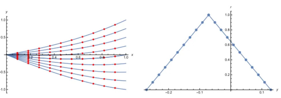
Figure 1: Left: Solutionsy1r(x) and y2r(x) for different values ofr;

Right:The exact and the numerical solutions atx= 0.2

y′′

1r(x) = y

′

2r(x) + 2−r, y

′′

2r(x) =y

′

1r(x) +r

y1r(0) = 0, y2r(0) = 0; y1r(1) =r−1, y2r(1) = 1−r.

y′′

1r(x) = y

′

1r(x) + 2−r, y

′′

2r(x) =y

′

2r(x) +r

y1r(0) = 0, y2r(0) = 0; y1r(1) =r−1, y2r(1) = 1−r.

y′′

1r(x) = y

′

2r(x) +r, y

′′

2r(x) =y

′

2r(x) + 2−r

y1r(0) = 0, y2r(0) = 0; y1r(1) =r−1, y2r(1) = 1−r.

To implement the shooting method, we first rewrite each system as a first order initial value system then solve the initial value problems involved using the FIRK. The solutions corresponding to the 1 - 1 differentiability for different values of r = 0.0, 0.25, 0.5, 0.75, 1.0 are given in Figure 1 (left). Note that the upper 4 curves are fory1r(x) and the lower 4 curves are fory2r(x) with

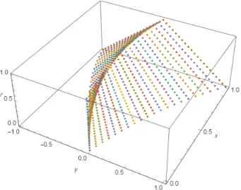
the middle for both at r = 1 since they coincide. Figure 1 (right) shows the solution at x = 0.2 of both the exact and the approximate numerical one. In Figure 2 we present a 3-D simulation of the solution.

(11)

Figure 2: 3-D simulation of the Solution

y′′

= y′

+ 3y+f(x)

y(0) =

2

9(r−1), 2

9(1−r)

y(1) =

2

9(r−1), 2

9(1−r)

with

f1r(x;r) = (1−r)(3−2t)−

1 3 9t

2₋_9t_{+ 2}

(1−r)

f2r(x;r) = (r −1)(3−2t)−

1 3(9t

2₋_9t_{+ 2)(r} ₋_1).

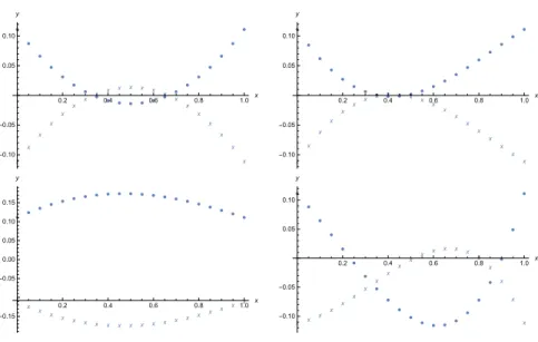
The solutions of the (1−1), (1 −2), (2 −1) and (2−2) systems for r = 0.5 are given in Figures 3. The results obtained match with that reported in Glufatullayev et al. [6].

References

(12)

x x x x x x x x

x x x x x _x

x x x x x x x

0.2 0.4 0.6 0.8 1.0x

-0.10 -0.05 0.05 0.10 y x x x x x x x

x x x x _x

x x x x x x x x x

0.2 0.4 0.6 0.8 1.0 x

-0.10 -0.05 0.05 0.10 y x x x _x x _x

x x x x x x x x x x x x

x x

x

0.2 0.4 0.6 0.8 1.0x

-0.15 -0.05 0.00 0.05 0.10 0.15 y x x x x x x x x x x x x

x x x _x

x

0.2 0.4 0.6 0.8 1.0 x

-0.10

-0.05 0.05 0.10

y

Figure 3: The solutions of the (1-1), (1-2), (2-1) and (2-2) systems forr= 0.5.

[2] B. Attili, On the numerical implementation of the shooting methods to the one-dimensional singular boundary value problems,Intern. J. Comput. Math.,47 (1993), 65-75.

[3] B. Bede, I. Rudas and A. Bencsik, First order linear fuzzy differential equa-tions under generalized differentiability, Inform. Sci., 177 (2007), 1648-1662.

[4] Y. Chalco-Cano, and H. Roman-Flores, On new solution of fuzzy differen-tial equations, Chaos, Solit. Fract.,38(2008), 112-119.

[5] O. Fard, T. Bidgoli and A. Rivaz, On existence and uniqueness of solutions to the fuzzy dynamic equations on time scales, Math. Comput. Appl., 22 (2017), 1-16.

[6] A. G. Fatullayev, E. Can and C. Koroglu, Numerical solution of a boundary value problem for a second order fuzzy differential equation,TWMS J. Pure Appl. Math.,4 (2013), 169-176.

(13)

[8] E. Hullermeier, An approach to modeling and simulation of uncertain dy-namical systems,Inter. J. Uncertain. Fuzz. and Knowledge Based Syst.,5 (1997), 117-137.

[9] R. Jafari, W. Yu, Xiaoou Li and S. Razvarz, Numerical solution of fuzzy differential equations with Z-numbers using Bernstein neural networks, In-tern. J. Comput. Intelli. Sys.,10 (2017) 1226-1237.

[10] O. Kaleva, Fuzzy differential equations,Fuzzy Sets and Systems,24(1987), 301-317.

[11] H.B. Keller, Numerical Solution of Two Point Boundary Value Problems, SIAM (1976).

[12] A. Khastan and K. Ivaz, Numerical solution of fuzzy differential equations by Nystrom method,Chaos, Solit. Fract.,41(2009), 859-868.

[13] A. Khastan, and J. Nieto, A boundary value problem for second order fuzzy differential equations,Nonlinear Anal., 72(2010), 3583-3593. [14] V. Lakshmikantham, K. Murty and J. Turner, Two point boundary value

problems associated with nonlinear fuzzy differential equations,Math. In-equal. and Applic.,4 (2001), 527-533.

[15] D. Li, M. Chen and X. Xue, Two point boundary value problems of un-certain dynamical systems,Fuzzy Sets and Systems,179 (2011), 50-61. [16] D. O’Regan, V. Lakshmikantham and J. Nieto, Initial and boundary value

problems for fuzzy differential equations, Nonlin. Anal., 54 (2003), 405-415.

[17] S. Palligkinis, G. Papageorgiou and I. Famelis, Runge-Kutta methods for fuzzy differential equations,Appl. Math.and Comput.209 (2009), 97-105. [18] F. Rabiei, F. Ismail, N. Senu and N. Abasi, Construction of improved Runge-Kutta Nystrom method for solving second order ordinary differen-tial equations, World Appl. Sci. J. 20(2012), 1685-1695.

[19] F. Rabiei, F. Abd Hamid, M. Rashidi and F. Ismail, Numerical simulation of fuzzy differential equations using general linear method and B-series,

Advanc. in Mech. Eng.,9 (2017), 1–16.

(14)