Chasing Hard-to-Get Cases in Panel
Surveys: Is it Worth it?
Nicole Watson & Mark Wooden
Melbourne Institute of Applied Economic and Social Research,
University of Melbourne
Abstract
In many population surveys, fieldwork effort tends to be disproportionately concentrated on a relatively small proportion of hard-to-get cases. This article examines whether this effort is justified within a panel survey setting. It considers three questions: (i) are hard-to-get cases that are interviewed different from other interviewed cases? (ii) do cases that require a lot of effort in one survey wave require a lot of effort in all waves? and (iii) can easy-to-get cases be re-weighted to eliminate biases arising from not interviewing hard-to-get cases? Using data from a large nationally representative household panel survey, we find that hard-to-get cases are distinctly different from easy-to-get cases, suggesting that failure to obtain interviews with them would likely introduce biases into the sample. Further, being hard-to-get is mostly not a persistent state, meaning these high cost cases are not high cost every year. Simulations confirm that removing hard-to-get cases introduces biases, and these biases lead to an understatement of the extent of change experienced by the population. However, we also find that under one of five fieldwork curtailment strate-gies considered, the bias in population estimates that would arise if the hard-to-get cases were not pursued can be corrected by applying weights. Nevertheless, this conclusion only applies to the curtailment strategy involving the smallest decline in sample size. Biases associated with curtailment strategies involving larger sample size reductions, and hence greatest cost savings, are not so easily corrected.
Keywords: HILDA Survey, sample representativeness, longitudinal surveys, fieldwork
curtailment strategies, fieldwork efficiency
© The Author(s) 2019. This is an Open Access article distributed under the terms of the
Acknowledgments
The research reported on in this paper was, in part, supported by an Australian Re-search Council Discovery Grant (#DP1095497). This paper uses unit record data from the Household, Income and Labour Dynamics in Australia (HILDA) Survey. The HILDA Project was initiated and is funded by the Australian Government Department of Social Services (DSS) and is managed by the Melbourne Institute of Applied Eco-nomic and Social Research (Melbourne Institute). The findings and views reported in this paper, however, are those of the authors and should not be attributed to either DSS or the Melbourne Institute.
Direct correspondence to
Nicole Watson, Melbourne Institute of Applied Economic and Social Research, Level 5, 111 Barry Street, University of Melbourne, Victoria 3010, Australia E-mail: [email protected]
The return to additional survey fieldwork effort, as measured by additional sur-vey respondents, invariably declines with the rate of response. Obtaining very high response rates to population surveys thus typically requires concentrating field-work effort, especially towards the end of the fieldfield-work period, on a relatively small proportion of cases who are hard-to-get. But is the extra effort and cost spent on achieving high response rates justified?
or not pursuing cases extend well beyond a single wave. In this article, we examine whether the fieldwork effort devoted to obtaining hard-to-get interviews across six annual survey waves is justified.
Another feature of previous research using either cross-sectional or panel data is the wide variation across studies in how a ‘hard-to-get’ case is defined. The most common types of definitions employed include any case that: requires a large num-ber of numnum-ber of visits or calls (Cottler et al., 1987; Hall et al., 2013; Heerwegh et al., 2007; Kennickell, 2000; Lin & Schaeffer, 1995; Lynn et al., 2002; Yan et al., 2004); has refused earlier in the fieldwork period (Billiet et al., 2007; Hall et al., 2013; Fitzgerald & Fuller, 1982; Lin & Schaeffer, 1995; Lynn et al., 2002; Woodruff et al., 2000; Yan et al., 2004); or was interviewed late in the fieldwork period (Etter & Perneger, 1997; Haring et al., 2009; Kennickell, 2000; Lahaut et al., 2003; Lar-roque et al., 1999; Studer et al., 2013; Ullman & Newcomb, 1998; Yan et al., 2004).
Most studies find that hard-to-get cases are different from easy-to-get cases. These differences extend from socio-demographic variables such as age (Cottler et al., 1987; Hall et al., 2013; Kennickell, 2000; Larroque et al., 1999), sex (Cottler et al., 1987), race (Cottler et al., 1987; Hall et al., 2013), and education (Cottler et al., 1987; Etter & Perneger, 1997; Kennickell, 2000; Larroque et al., 1999), to more substantive variables such as employment (Hall et al., 2013), occupation (Larroque et al., 1999), income (Etter & Perneger, 1997; Kennickell, 2000), wealth (Kennick-ell, 2000), smoking (Woodruff et al., 2000), substance use (Studer et al., 2013), and physical health (Etter & Perneger, 1997). Obtaining interviews with these hard-to-get cases is expected to reduce biases in survey estimates. How important this reduction in bias is, however, depends on how similar the interviewed hard-to-get cases are to the non-respondents.
For longitudinal surveys, decisions about how much effort to devote to pursu-ing hard-to-get cases should be influenced, at least in part, by expectations about the likelihood of retaining such sample members in subsequent waves. Being a hard-to-get respondent in one wave, for example, has been found to be predictive of attrition in the next (Haring et al., 2009; Watson & Wooden, 2009). More gener-ally, does the extra effort (and cost) required to interview the hard-to-get cases fall persistently on the same cases from wave to wave? As far as we are aware, this is an issue not considered in any previous research.
Further, and perhaps most importantly, relatively few studies have tested in a simulation setting whether re-weighting the easy-to-get cases can reduce the poten-tial biases introduced from not pursuing interviews with the hard-to-get cases. And those studies that have been conducted (e.g., Billiet et al., 2007; Hall et al., 2013) have used cross-sectional data.
1. Are hard-to-get cases that are ultimately interviewed different from other inter-viewed cases?
2. Do cases that require a lot of effort in one survey wave require a lot of effort in all waves?
3. Can easy-to-get cases be re-weighted to eliminate biases potentially arising from not interviewing hard-to-get cases?
We build on previous research in a number of ways. First, we define hard-to-get cases in five different ways and so can assess how sensitive conclusions are to the choice of measure. Second, we analyze the extent to which being hard-to-get is a state that persists over time. Third, we examine whether the biases that may result if fieldwork is curtailed over an extended period (six annual survey waves) can be eliminated by re-weighting the remaining (i.e., easy-to-get) cases.
Data
The HILDA Survey is a panel that began in 2001 with a three-stage stratified clus-tered nationally representative sample of households (Watson & Wooden, 2012). There were 19,914 people living in the 7682 responding households in wave 1. These people are followed over time and the sample is extended to include all people liv-ing with these original sample members at the time of the subsequent interviews. Interviews are conducted annually with all sample members aged 15 years or older. The vast majority (over 90 percent) of these interviews are undertaken face-to-face, with the remainder by telephone.
The initial responding sample was achieved from a total of 11,693 households identified as in-scope, giving a wave 1 household-level response rate of 66 percent (AAPOR RR1). Annual re-interview rates of individuals are high, rising from 87 percent in wave 2 to over 94 percent by wave 5, and remaining above that level in all subsequent waves.
Methods
Defining Hard-to-Get Cases
We examine a range of different definitions of ‘hard-to-get’, based on the length of time since commencement of fieldwork, whether an initial refusal was received, and the number of calls made. The most natural delineations of time for the HILDA Survey are the fieldwork stages described earlier, with the survey manager deciding at the end of the first and second fieldwork stages who among the non-respondents should be re-approached. The two time-based definitions of hard-to-get cases used here are:
Definition A: The individual was interviewed during a follow-up stage of field-work.
Definition B: The interview was completed after the New Year.
Alternatively, the survey manager may choose not to re-issue to field anyone who initially refused. This suggests a third definition:
Definition C: The individual initially refused before being interviewed.
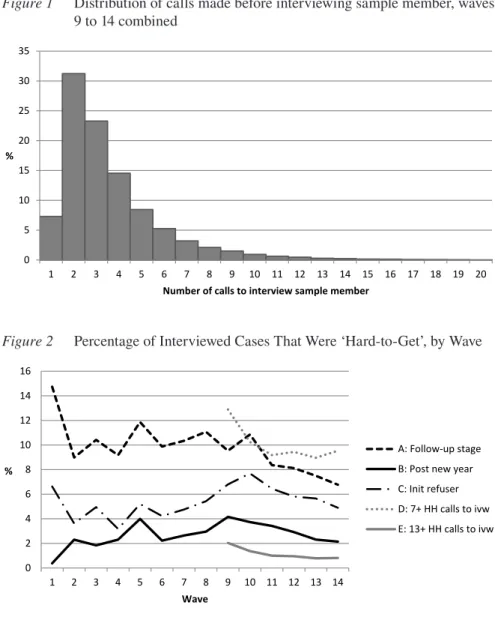
Finally, we create binary variables based on the number of calls exceeding some threshold. A call is counted if it was a face-to-face visit or if it was a telephone call that resulted in an appointment, an interview, or other information to finalize the outcome of an individual. From 2009 (wave 9), a change from pen-and-paper interviewing to computer-assisted personal interviewing facilitated the collection of detailed call records. Using these records, we can determine the number of calls made to the household before a particular individual is interviewed. The distribu-tion of these calls, based on data pooled from waves 9 to 14, is shown in Figure 1. For this analysis, we focus on two specific thresholds – 7 or more calls, and 13 or more calls required to obtain an interview. Obviously, a number of different thresh-olds could have been selected due to the greater granularity of call-based measures compared to those used in the first three definitions. The choice of the particular thresholds used here reflects the operational requirements imposed on the company engaged to undertake the fieldwork for the HILDA Survey. Specifically, an inter-viewer must make at least six calls to a household in a particular fieldwork period before they can return the household to the office with an inconclusive outcome (such as a non-contact), and then up to a further 6 calls after making contact to interview sample members. This provides two further definitions.
Definition D: 7 or more calls were made to the household by the time the indi-vidual was interviewed.
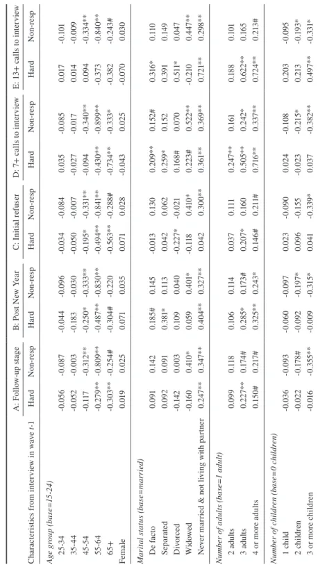
Figure 2 shows the proportion of interviews that were hard-to-get according to each of these five definitions, and how this has varied over time. Approximately 10 per-cent of interviews required a follow-up period of fieldwork to achieve the interview (definition A); though there is a noticeable decline in this proportion in later waves (waves 11 to 14). Only about half of these follow-up cases were due to an initial refusal (definition C) in the early waves, but this rises to around 70 percent in waves 9 to 14. This shift coincides with a change in fieldwork provider, which occurred
Figure 1 Distribution of calls made before interviewing sample member, waves 9 to 14 combined
0 5 10 15 20 25 30 35
1 2 3 4 5 6 7 8 9 10 11 12 13 14 15 16 17 18 19 20
%
Number of calls to interview sample member
Figure 2 Percentage of Interviewed Cases That Were ‘Hard-to-Get’, by Wave
0 2 4 6 8 10 12 14 16
1 2 3 4 5 6 7 8 9 10 11 12 13 14
%
Wave
after wave 8, suggesting either a change in re-issuing practice or a greater ability on the part of the new provider to convert initial refusals to interviews. The propor-tion of cases interviewed after the New Year (definipropor-tion B) each wave is relatively small (2 to 4 percent) and varies somewhat wave to wave. The proportion of cases defined as hard-to-get when using call counts varies substantially depending on the particular call threshold applied. Using a cut-off of 7 or more calls to define a hard-to-get case (definition D) results in 9 to 13 percent of the interviewed cases being classified as hard-to-get. When the higher cut-off of 13 or more calls is used (definition E), the proportion of interviewed cases defined as hard-to-get declines to just 1 to 2 percent.
Assessing the Impact of Pursuing Hard-to-Get Cases
Multinomial logistic models of the three interview outcomes at wave t – easy-to-get interview, hard-to-get interview, and not interviewed – are used to assess whether the hard-to-get cases are appreciably different from the easy-to-get cases (research question 1). We include a range of personal and household characteristics, all mea-sured at wave t-1, that are often found to be associated with non-response (see Wat-son & Wooden, 2009). These include: age (in 10-year bands), sex, marital status (6 categories), number of adults living in the household, number of children (aged less than 15) living in the household, education level (6 categories), country / region of birth (3 categories), whether the sample member has a restrictive long-term health condition, area of residence (9 categories), employment status (6 categories), real equivalized (i.e., household size adjusted) gross annual (financial year) household income (with missing values imputed; see Hayes & Watson, 2009), whether an owner-occupier of a home, whether the household moved between waves t-1 and t, and a set of wave indicators.
Missing data on covariates resulted in the loss of just 520 observations (0.7 percent) from the models employing the first three definitions of hard-to-get, leav-ing a total of 77,315 person-wave observations. For the last two hard-to-get defi-nitions, a further 54 person-wave observations were dropped due to missing call record information. To allow repeated observations on the same individuals, the multinomial logistic models are fitted as two-level hierarchical models where level 1 is the wave observation and level 2 is the individual. Two random effects, which were allowed to be correlated, were assumed for the different interview outcomes.
To assess whether individuals are hard-to-get repeatedly over time simply because of their particular socio-demographic characteristics (research question 2), we rerun the above set of multinomial logit models and include an indicator vari-able for whether the individual was hard-to-get in wave t-1.
sample curtailment strategies are associated with significant differences in selected personal and household characteristics, and assess whether these differences can be eliminated through the application of survey weights constructed for the reduced sample under each of the five curtailment strategies that only contains the easy-to-get cases. We then similarly test for differences in responses to 15 selected esti-mates of change over time. The weights used relate to a “balanced” panel of respon-dents from wave 1 to 14 where the hard-to-get cases have been dropped from wave 9 onwards. The balanced panel weights were constructed by adjusting the wave 1 cross-sectional weights for attrition from wave 1 to wave 14 (by multiplying by the inverse of the response propensity that is modelled on a range of wave 1 socio-economic characteristics and some post-wave 1 mobility information where avail-able). The weights are then calibrated to a set of external wave 1 totals. This follows the same methodology employed to construct the regular HILDA Survey weights (Watson, 2012). Standard errors of the difference between the full sample and the truncated sample (i.e., after excluding the hard-to-get cases) for each definition of hard-to-get, were calculated using jackknife estimation with 45 replicates.
To ensure that all definitions are examined across the same timeframe, all analyses that follow are restricted to the outcomes observed in waves 9 to 14.
Results
Are the Hard-to-Get Cases Different From Other Cases?
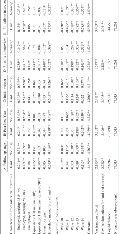
The coefficients from the estimation of multinomial logit regression models with random effects predicting interview outcomes are shown in Table 1. Separate esti-mates are provided for each of the five definitions of hard-to-get.
Ta bl e 1 M ul tin om ia l L og it o f I nt er vi ew O ut co me , w ith R an do m E ffe ct s: w av
es 9 t
o 1 4 A : F ol lo w-up st ag e B: P ost N ew Y ea r C: In iti al re fuser D : 7 + c al ls t o i nt er vi ew E: 1 3+ c al ls t o i nt er vi ew Ch ar ac te rist ic s f ro m i nt er vi ew i n w av e t-1 H ar d N on -re sp H ar d N on -re sp H ar d N on -re sp H ar d N on -re sp H ar d N on -re sp Ag e g ro up ( ba se =1 5-24 ) 25 -34 -0.0 56 -0.0 87 -0.0 44 -0.0 96 -0.0 34 -0.0 84 0.0 35 -0.0 85 0.0 17 -0 .10 1 35 -4 4 -0.0 52 -0.0 03 -0. 183 -0.0 30 -0.0 50 -0.0 07 -0.0 27 -0.0 17 0.0 14 -0.0 09 45 -5 4 -0 .11 7 -0 .31 2* * -0 .2 50* -0 .333 ** -0 .19 5* -0 .3 31* * -0.0 94 -0 .3 40 ** 0.0 94 -0 .3 34* * 55 -6 4 -0 .2 79 ** -0 .8 09 ** -0.4 87 ** -0. 83 0* * -0 .49 4** -0 .8 41* * -0.4 30 ** -0 .8 99 ** -0 .3 73 -0 .8 40 ** 65+ -0 .3 03 ** -0. 25 4# -0. 30 4# -0. 22 0 -0 .5 63 ** -0. 28 8# -0 .73 4* * -0 .333 * -0 .38 2 -0 .2 43 # Fe m al e 0.0 19 0.0 25 0.0 71 0.0 35 0.0 71 0.0 28 -0.0 43 0.0 25 -0.0 70 0.0 30 M ar ita l s ta tu s ( ba se= m ar ri ed ) D e fa ct o 0.0 91 0.14 2 0.18 5# 0.14 5 -0.0 13 0.1 30 0. 20 9** 0.1 52 # 0. 31 6* 0.11 0 Sep ar at ed 0.0 92 0.0 91 0. 38 1* 0.11 3 0.0 42 0.0 62 0. 259 * 0.1 52 0. 391 0.14 9 D iv or ce d -0 .14 2 0.0 03 0.1 09 0.0 40 -0 .227 * -0.0 21 0.1 68 # 0.0 70 0. 51 1* 0.0 47 W id ow ed -0 .16 0 0.4 10 * 0.0 59 0.4 01 * -0 .11 8 0.4 10 * 0. 223 # 0. 52 2* * -0 .2 10 0.4 47 ** N ev er m ar rie
d & n
A : F ol lo w-up st ag e B: P ost N ew Y ea r C: In iti al re fuser D : 7 + c al ls t o i nt er vi ew E: 1 3+ c al ls t o i nt er vi ew Ch ar ac te rist ic s f ro m i nt er vi ew i n w av e t-1 H ar d N on -re sp H ar d N on -re sp H ar d N on -re sp H ar d N on -re sp H ar d N on -re sp H ig he st l ev el o f e du ca tio n ( ba se =Y ea r 1 1 o r b el ow ) Ye ar 1 2 0.1 03 # -0 .13 4 -0.0 36 -0 .17 6* 0.0 25 -0 .14 4 0.0 78 -0 .15 3# -0 .12 4 -0 .17 3* Ce rt I II o r I V 0.0 83 -0.0 72 0.0 94 -0.0 85 0.0 39 -0.0 77 0.1 20 * -0.0 62 -0 .13 6 -0.0 96 D ip lo m a 0.0 25 -0 .2 68* -0 .16 3 -0 .31 1* -0.0 51 -0 .2 91* 0.0 48 -0 .2 60* 0.0 79 -0 .2 75 * G rad ua te -0 .15 4* -0 .4 49 ** -0 .2 90* -0 .49 1** -0 .3 75 ** -0 .49 2** -0 .12 7* -0.4 35 ** -0.4 64 ** -0.4 57 ** Po st g rad ua te -0 .18 2* -0 .6 25* * -0. 22 6# -0 .6 40 ** -0 .3 65* * -0 .6 59 ** -0 .2 20* * -0 .6 29* * -0.4 11 * -0 .6 06* * Cou nt ry o f b ir th (b as e= Au st ra lia ) M ai n E ng lis h-sp ea ki ng co unt ry -0.0 34 -0 .13 0 -0 .13 0 -0 .15 2 -0 .14 3 -0 .15 7 -0.0 17 -0 .14 0 -0.0 34 -0 .14 3 N ot m ai n E ng lis h-sp ea ki ng co unt ry 0.4 16 ** 0. 37 7* * 0.4 32 ** 0. 35 0* * 0. 27 1* * 0. 33 8* * 0.4 31 ** 0. 38 2* * 0. 53 7* * 0. 305 ** Lo ng t er m h ea lth c on di tio n -0 .11 4* -0.0 10 -0 .2 69 ** -0.0 09 -0 .139 ** -0.0 23 -0 .12 7* * -0.0 15 -0 .2 15 # -0.0 11 Ar ea o f r es id en ce ( ba se = M aj or c ity : S yd ne y) M aj or c ity : M el bo ur ne -0 .16 4* -0 .18 7# -0 .2 57* -0 .17 0 -0 .16 8* -0 .18 5# -0 .13 1* -0 .19 7# -0 .3 05 * -0 .16 9# M aj or c ity : B ris ba ne -0.0 86 -0 .16 1 -0. 20 4 -0 .16 0 -0 .18 5# -0 .18 7 -0 .6 67* * -0 .2 77* -1 .10 5* * -0 .17 9 M aj or c ity : A de la id e -0.0 62 -0.0 82 -0 .19 7 -0.0 95 -0 .18 6# -0.0 99 -0 .5 21* * -0 .17 5 -1 .5 63 ** -0 .12 1 M aj or c ity : P er th -0 .10 8 0.0 72 -0 .2 15 0.0 71 -0 .2 71* 0.0 22 -0 .2 96* * 0.0 16 -0 .52 7* * 0.0 58 M aj or c ity : o th er -0.4 23 ** -0.4 78 ** -0.4 16 ** -0.4 70 ** -0 .5 45* * -0.4 87 ** -0 .8 55* * -0 .58 0** -1. 13 4* * -0.4 59 ** Inn er re gi on al -0.0 48 -0 .10 9 -0 .32 6* * -0 .13 7 -0 .16 5* -0 .131 -0 .6 80 ** -0 .2 50* * -1 .0 41* * -0 .151 O ut er re gio na l 0.18 2* 0. 30 1* * 0. 20 2# 0. 26 4* 0.0 26 0. 27 0* -0 .72 2* * 0.1 31 -0 .72 7* * 0. 26 2* Re m ot e 0. 629* * 0. 68 6* * 1.0 04* * 0. 69 9** 0. 60 8* * 0. 69 4* * -0. 20 5# 0. 49 8** -0. 30 8 0. 53 6* * Em pl oy m en t s ta tu s ( ba se = no t i n l ab ou r f or ce ) Em pl oy ed , w or ki ng < =3 4 h rs -0.0 57 -0 .12 7 -0 .100 -0 .11 4 -0.0 06 -0 .133 0.1 00 * -0 .12 5 0.1 21 -0 .12 8 Em pl oy ed , w or ki ng 3 5-44 h rs 0.0 87 0. 26 4* * 0.14 3 0. 27 0* * 0. 20 8* * 0. 252 ** 0.1 34 * 0. 27 3* * 0. 36 5* 0. 26 9** Ta bl
e 1 c
on
tinu
A : F ol lo w-up st ag e B: P ost N ew Y ea r C: In iti al re fuser D : 7 + c al ls t o i nt er vi ew E: 1 3+ c al ls t o i nt er vi ew Ch ar ac te rist ic s f ro m i nt er vi ew i n w av e t-1 H ar d N on -re sp H ar d N on -re sp H ar d N on -re sp H ar d N on -re sp H ar d N on -re sp Em pl oy ed , w or ki ng 4 5-54 h rs 0. 20 4* * 0. 32 1* * 0. 24 1* 0. 31 3* * 0. 30 8* * 0. 31 9* * 0. 25 5* * 0. 34 2* * 0.4 24 * 0. 33 1* * Em pl oy ed , w or ki ng 5 5+ h rs 0.4 80 ** 0. 60 9** 0. 38 1* * 0. 56 4* * 0. 54 2* * 0. 58 8** 0.4 41 ** 0. 58 7** 0. 56 8* * 0. 57 0* * Une mp lo ye d 0.0 18 0. 23 8# 0.0 66 0. 24 6* 0.14 3 0. 23 5# 0.1 52 # 0. 257* 0.18 6 0. 26 1* Eq ui va liz ed H H i nc om e ( /1 0 5) 0.4 35 ** 0.1 51 0.4 02 ** 0.1 81 0. 38 2* * 0.1 68 0.4 43 ** 0.1 57 0. 317 0.1 25 Eq ui va liz ed H H i nc om e s qu ar ed ( /1 0 10) -0 .0 49 ** -0.0 03 -0.0 46 -0.0 08 -0.0 38 # -0.0 05 -0.0 71 ** -0.0 04 -0.0 91 -0.0 02 O w ne r o cc up ie r 0.0 15 -0 .10 3 -0.0 14 -0.0 97 0.0 33 -0.0 94 -0 .14 8* * -0 .13 2* -0 .2 67* -0 .12 1# H ou se ho ld m ov ed ( bt w t -1 a nd t ) 0. 53 3* * 0.4 19 ** 0. 839 ** 0.4 18 ** 0. 60 5* * 0.4 26 ** 0. 50 2* * 0. 39 8** 0. 575 ** 0. 32 2* * Ne xt w av e ( ba se = w av e 9 ) Wa ve 10 0. 30 3* * 0.18 0* 0.0 65 0.11 3 0. 28 6* * 0.1 68 * -0 .2 18 ** 0.0 58 -0.4 20 ** 0.0 96 W av e 11 0.0 20 0.17 0* 0.0 67 0.1 68 * 0.1 55 * 0. 20 1* -0 .3 07* * 0.1 04 -0.4 85 ** 0.1 59 * W ave 12 0.0 53 0. 339 ** -0.0 61 0. 31 9* * 0.111 # 0. 358 ** -0 .19 8* * 0. 28 9** -0 .5 18 ** 0. 32 0* * Wa ve 1 3 -0.0 19 0. 37 3* * -0 .18 8* 0. 36 2* * 0.1 24 * 0.4 10 ** -0 .222 ** 0. 32 8* * -0 .58 2** 0. 36 7* * Wa ve 14 -0 .11 5* 0. 34 4* * -0 .3 02* * 0. 339 ** -0.0 22 0. 37 7* * -0 .14 3* * 0. 33 1* * -0 .58 5** 0. 35 4* * Co ns ta nt -3 .4 89 ** -4 .70 3* * -4 .9 39 ** -4 .73 2* * -3 .76 6* * -4 .71 9* * -2 .73 4* * -4 .52 6* * -5 .6 75 ** -4 .5 94* * Va r ( ra nd om e ffe ct s) 2.1 55 ** 3. 20 2* * 2. 41 1* * 1. 54 7* * 3. 40 3* * Co v ( ra nd om e ffe ct s f or h ar d a nd n on -re sp ) 2.7 28 ** 3. 49 6** 3. 00 3* * 2.1 81 ** 3. 04 1* * Lo g-lik eli ho od -2 9,6 94 -18 ,8 90 -2 5, 83 2 -31 ,8 52 -14 ,75 3 N( pe rs on -y ea r o bs er vat io ns ) 77, 31 5 77, 31 5 77, 31 5 77 ,26 1 77 ,26 1 No te
: # p<
0.1
0; * p<
0. 05 ; * * p< 0. 01 . Ta bl
e 1 c
on
tinu
How Persistent are Hard-to-Get Cases?
Do cases that require a lot of work in one wave require a lot of work in all waves? Figure 3 shows the proportion of hard-to-get cases at one wave that are interviewed in subsequent waves but were hard-to-get. It shows that the level of reoccurrence is relatively low, with 9 to 24 percent of hard-to-get cases in one wave classified as to-get in the next wave, and the rate of persistence in being classified as hard-to-get declines over time, with 5 to 17 percent classified as hard-hard-to-get four waves later. The large majority (75 to 90 percent, depending on the hard-to-get definition used) of hard-to-get cases are classified as easy-to-get in the next wave.
Does the relatively small amount of persistence observed in the hard-to-get cases remain after controlling for respondent characteristics? To test this, we mod-ify the model presented in Table 1 (which predicts whether a case will be easy-to-get, hard-to-get or a non-respondent) and include an indicator of whether the indi-vidual was hard-to-get in the prior wave (when the other characteristics included in the model were measured). Table 2 reports the estimated coefficients and mean pre-dicted probabilities for this variable. We find a strong negative association between being hard-to-get in one wave and being easy-to-get in the next. The predicted probability, holding all else constant, of being an easy-to-get case (using definition A; i.e., whether they require follow-up work or not) for those who were easy-to-get in the previous wave is 89.1 percent. This compares with 80.9 percent of those who were previously hard-to-get. The differences in the predicted probabilities are similar for the other four definitions; i.e., 7.2 percentage points for definition B, 8.4 percentage points for definition C, 8.3 percentage points for definition D, and 6.5 percentage points for definition E.
In summary, the large majority of hard-to-get cases (over 80 percent under all definitions) are easy-to-get come the next survey wave. This is not to say, however, that there is no state persistence; a hard-to-get case is still much more likely (around twice as likely) to be hard-to-get next wave than an otherwise comparable case clas-sified as easy-to-get.
Can the Differences in Hard-to-Get Cases be Corrected by
Weighting?
Figure 3 Average Percentage of Hard-to-Get Interviewed Cases in Future Waves Conditional on Being Hard-to-Get in Wave t
0 5 10 15 20 25
t+1 t+2 t+3 t+4
%
hard-to-get
cases
Wave
A: Follow-up stage B: Post new year C: Init refuser D: 7+ HH calls to ivw E: 13+ HH calls to ivw
Table 2 Coefficient and Predicted Probabilities for Hard-to-Get in Prior Wave in Multinomial Logit Model of Interview Outcome with Random Effects
Easy-to-get at t Non-respondent at t Mean predicted
probability Mean predicted probability
Hard-to-get in wave t-1 Coeff at Hard t-1 at Easy t-1 Coeff Hard at t-1 atEasy t-1 Definition A: Follow-up stage -0.800** 80.9 89.1 0.059 6.9 4.0 Definition B: Post New Year -1.205** 86.2 93.4 -0.238* 7.9 4.2 Definition C: Initial refuser -0.936** 82.4 90.8 0.003 7.3 4.1 Definition D: 7+ calls to interview -0.714** 80.2 88.4 0.181* 6.9 3.8 Definition E: 13+ calls to interview -1.315** 88.5 95.0 -0.188 9.2 4.2
Note: Models include controls for all the covariates shown in Table 1. # p<0.10; * p<0.05;
** p<0.01.
panel. The full balanced panel from wave 1 to 14 includes 6707 individuals. This declines to 6572 when cases requiring 13 or more calls (definition E) are excluded (a 2 percent reduction), or 6245 cases if the post New Year fieldwork (definition B) is dropped (a 7 percent reduction). Greater reductions in the sample occur when the broader definitions of hard-to-get are used. The balanced panel contains 5661 cases if all initial refusers (definition C) are dropped (a 16 percent reduction), 5225 cases if all follow-up fieldwork (definition A) is abandoned (a 22 percent reduction), or 5046 cases if cases requiring 7 or more calls (definition D) are dropped (a 25 percent reduction).
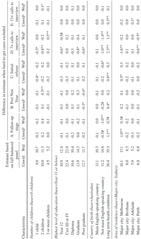
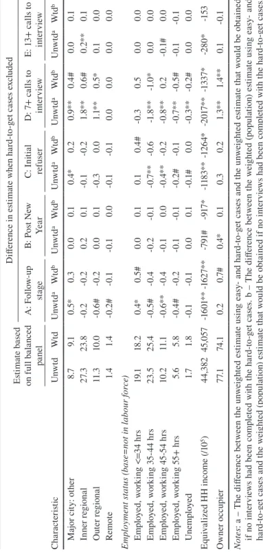
The unweighted and weighted estimates for the personal and household vari-ables for the full balanced panel are presented in the first two columns of Table 3. The weighted estimates are constructed by weighting the responses provided by both easy- and hard-to-get cases by the wave 1 to 14 balanced panel weight available in the HILDA Survey dataset. The unweighted estimates are similarly restricted to cases that have a positive balanced panel weight to aid comparison of the weighted and unweighted estimates. The following columns in the table provide (for each definition of hard-to-get): i) the difference between the unweighted estimate for the full balanced panel and the unweighted estimate obtained after dropping the relevant hard-to-get cases from waves 9 to 14; and ii) the difference between the weighted estimate for the full balanced panel and the estimate obtained by apply-ing the recalculated balanced panel weight after droppapply-ing the relevant hard-to-get cases from waves 9 to 14. The estimates are marked to indicate the p-value for the two-sided z-test for whether this difference is statistically different from zero (# p<0.10; * p<0.05; ** p<0.01).
We find that the definition of hard-to-get that shows the largest number of dif-ferences in the unweighted estimates is the curtailment strategy that drops the most cases (definition D which drops cases requiring 7 or more calls) and is least able to be corrected by the weights. The curtailment strategy affecting the personal and household estimates the least is definition E, which drops people requiring 13 or more calls. Further, these estimates are most amenable to correction by the appli-cation of weights (while one estimate is not corrected, this is expected by chance alone). Nevertheless, this strategy involves a very small decline in the number of cases followed, and hence the potential for costs savings is commensurately small. Arguably, our results suggest that the best curtailment strategy in terms of maxi-mising sample reduction (and thus saving fieldwork effort) while minimaxi-mising the effect on estimates is strategy A (not pursuing persons into the follow-up fieldwork phase). However, application of weights is still unable to correct for differences observed on at least three variables (age, country of birth and income).
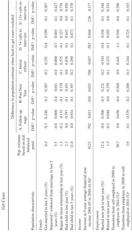
last five years; the proportion who separated from a marriage or were widowed in the last 5 years; the proportion that began a de facto relationship in the last year; the proportion who had a new birth in the last year; and the proportion who had a new birth in the last 5 years. There is one measure relating to income: the increase in the 5-year average income between the start and end of the panel (i.e., 2001-05 versus 2010-14). There are four estimates related to employment: whether a new job was started in the last year; whether retired in the last year; for those self-employed in 2009, the proportion that switched to being an employee by 2014; and for those who were employees in 2009, the proportion that transitioned to self-employment by 2014. In terms of health, we include the proportion of people who experienced the onset of a long-term health condition between 2009 and 2014. The final group of four estimates relate to housing: the proportion who moved house in the last year; the proportion who moved house in the last five years; the proportion who transitioned from living in a home that was not owned (i.e., was rented or provided rent-free) to one that was owned between 2009 and 2014; and the proportion who transitioned from living in a home that was owned to one that was not between 2009 and 2014.
The population estimates for the subset of variables are presented in the first column of Table 4. These estimates are constructed by weighting the responses pro-vided by easy- and hard-to-get cases (the full balanced panel) by the wave 1 to 14 balanced panel weight available in the HILDA Survey dataset. Subsequent columns in the table provide (for each definition of hard-to-get): i) the difference between this first population estimate and the one obtained by applying the recalculated bal-anced panel weight after dropping the relevant hard-to-get cases from waves 9 to 14; and ii) the p-value for the two-sided z-test for whether this difference is statisti-cally equivalent to zero.
Ta bl e 3 Es tim at es o f W av e 1 4 ( 20 14 ) P er so na l a nd H ou se ho ld C ha ra ct er ist ics a nd t he E ffe ct o f E xc lu di ng H ard-to -G et C as es Es tim at e ba se d on f ul l ba la nc ed pa ne l D iff er enc e i n e sti m at e w he n h ar d-to -g et c as es e xc lud ed A : F ol lo w-up sta ge B: P os t N ew Ye ar C: I ni tia l re fuser D: 7 + c al ls t o in te rv iew E: 1 3+ c al ls t o in te rv iew Ch ar ac te ris tic Unw td Wt d Unw td a Wt d b Unw td a Wt d b Unw td a Wt d b Unw td a Wt d b Unw td a Wt d b Ag e g ro up ( ba se =1 5-24 ) 25 -34 9.4 13 .9 -0 .5* * -0 .3* * -0 .5* * -0. 2# -0 .4* -0 .2* -0 .9 ** -0. 2 -0 .1 0.0 35 -4 4 16 .4 18 .9 -0 .4 -0 .4* -0. 2 -0 .1 -0 .9 ** -0. 3# -1 .3* * -0 .7* * -0 .1 -0 .1 45 -5 4 23 .3 20.6 0.1 0.4 0. 2 0. 2 -0. 2 0.4 # -1 .3* * 0. 2 -0. 2# 0.0 55 -6 4 21 .6 20 .1 0.0 0. 2 0. 2 0. 2 0. 3 0.1 -0 .1 0. 2 0.1 # 0. 2# 65+ 29. 4 26. 5 0. 8* 0.1 0. 3# -0 .1 1.1* * 0.1 3. 6* * 0. 5# 0. 2* * 0.0 Fe m al e 54. 6 51 .3 0.0 0.0 0.1 0.0 -0 .1 -0 .1 0.7 ** 0.1 0.0 0.0 M ar ita l sta tu s ( ba se = m ar ri ed ) D e fa ct o 9.7 10.6 -0. 2 -0. 2 -0 .1 -0 .1 -0 .1 0.1 -0 .9 ** -0 .7* 0.0 0.0 Sep ar at ed 3. 6 3. 4 0.0 0.0 0.0 0.0 -0 .1 -0 .1 -0. 3# -0. 2 0.0 0.0 D ivo rc ed 8. 5 7.6 0.1 0.0 0.1 0.1 0.0 -0 .1 -0 .1 -0. 3 0.0 0.0 W id ow ed 7.8 7.1 0.1 -0. 2 -0 .1 -0. 2 0.1 -0. 2 0.7 ** 0.0 0.1* * 0.0 N ev er m ar rie
d & n
Es tim at e ba se d on f ul l ba la nc ed pa ne l D iff er enc e i n e sti m at e w he n h ar d-to -g et c as es e xc lud ed A : F ol lo w-up sta ge B: P os t N ew Ye ar C: I ni tia l re fuser D: 7 + c al ls t o in te rv iew E: 1 3+ c al ls t o in te rv iew Ch ar ac te ris tic Unw td Wt d Unw td a Wt d b Unw td a Wt d b Unw td a Wt d b Unw td a Wt d b Unw td a Wt d b Nu m be r o f c hi ld re n ( ba se = 0 c hi ld re n) 1 c hi ld 9.8 10 .7 -0. 2 -0. 2 -0 .1 -0 .1 -0 .4* -0. 2 -0 .5* 0.0 -0 .1 0.0 2 c hi ldr en 10.0 11 .3 0. 2 0.4 0.1 0. 5* * -0. 2 0. 2 -0 .8* * -0. 2 0.1 0.1* 3 o r m or e c hi ld re n 4. 5 5. 2 0.0 0.1 -0 .1 -0 .1 -0. 2 0.0 0. 2 0. 5* * -0 .1 -0 .1 H ig he st l ev el o f e du ca tio n ( ba se =Y ea r 1
1 or b
el ow ) Ye ar 1 2 10 .9 12 .4 -0 .1 -0 .1 -0 .1 -0 .1 -0. 3 -0 .1 -0.6 * -0. 5# 0.0 0.0 Ce rt I II o r I V 22 .4 22 .9 -0 .1 0.0 0.0 0.0 -0. 3 -0. 2 0.0 0. 2 0.0 0.0 D ip lo m a 10.6 10 .4 -0. 2 -0 .1 0.1 0. 2 -0 .1 0.1 -0. 3 0.1 0.0 0.1 G rad ua te 13 .9 14 .3 0.0 -0. 2 0.1 0. 3 0.1 0.0 -0 .8* -0 .4 0.0 0.0 Po st g rad ua te 12 .7 11 .7 -0. 2 -0 .1 -0 .3* -0 .4* 0. 2 0.1 -0.6 * 0.1 0.0 0.0 C ou ntr y o f b ir th (ba se = Au str al ia ) M ai n E ng lis h-sp ea ki ng co unt ry 11 .1 10 .3 -0 .1 0.0 0.0 -0 .1 0.1 -0 .1 0.1 0.0 0.0 0.0 No t m ai n E ng lis h-sp ea ki ng co unt ry 11 .2 14 .8 -0. 5# -1 .0 ** -0. 2# 0.0 -0. 2 -0.6 * -1 .0 ** -1. 4* * 0.0 -0 .1 Lon g t er m h ea lth c on di tion 36 .4 35. 3 1.1* * 0.7 # 0. 4* 0. 2 0. 8* * 0. 3 2. 5* * 1.1* * 0. 3* * 0.1 Ar ea o f r es id en ce ( ba se = M aj or c ity : S yd ne y) M ajo r c ity : Me lb ou rn e 16 .1 17. 1 1.0 ** 0. 3# 0. 2 0.1 0. 5* 0. 3 -1 .6 ** -0. 2 -0. 2 0.0 M ajo r c ity : B ris ba ne 8.0 8. 3 -0. 2 0. 2 -0 .1 0.0 -0. 2 0. 2 0.1 0.0 0.0 0.0 M ajo r ci ty : A de la ide 5.9 5. 2 -0. 3 0.0 0.0 0.0 -0 .1 0.0 0.1 0.0 0.1* 0.0 M ajo r c ity : P er th 6.8 6.8 -0. 2 -0 .1 -0 .1 -0. 2 0.0 -0. 2 -0.6 ** -0 .5* 0.0 0.0 Ta bl
e 3 c
on
tinu
Es tim at e ba se d on f ul l ba la nc ed pa ne l D iff er enc e i n e sti m at e w he n h ar d-to -g et c as es e xc lud ed A : F ol lo w-up sta ge B: P os t N ew Ye ar C: I ni tia l re fuser D: 7 + c al ls t o in te rv iew E: 1 3+ c al ls t o in te rv iew Ch ar ac te ris tic Unw td Wt d Unw td a Wt d b Unw td a Wt d b Unw td a Wt d b Unw td a Wt d b Unw td a Wt d b M ajo r c ity : o th er 8.7 9.1 0. 5* 0. 3 0.0 0.1 0. 4* 0. 2 0.9 ** 0.4 # 0.0 0.1 In ne r r eg ion al 27. 3 23. 8 -0. 2 -0. 2 0. 2 0.1 -0 .1 -0. 2 1.8 ** 0.6 # 0. 2* * 0.1 O ut er r eg ion al 11 .3 10.0 -0.6 # -0. 2 0.0 0.1 -0. 3 0.0 1.1* * 0. 5* 0.1 0.0 Remo te 1.4 1.4 -0. 2# -0 .1 -0 .1 0.0 -0 .1 -0 .1 0.0 0.0 0.0 0.0 Em pl oy m en t s ta tu s ( ba se = no t i n l ab ou r f or ce ) Em pl oy ed , w or ki ng < =3 4 h rs 19. 1 18 .2 0. 4* 0. 5# 0.0 0.1 0.1 0.4 # -0. 3 0. 5 0.0 0.0 Em pl oy ed , w or ki ng 3 5-44 h rs 23. 5 25. 4 -0. 5# -0 .4 -0. 2 -0 .1 -0 .7* * -0.6 -1 .8 ** -1 .0 * 0.0 0.0 Em pl oy ed , w or ki ng 4 5-54 h rs 10 .2 11 .1 -0.6 ** -0 .4 -0 .1 0.0 -0 .4* * -0. 2 -0 .8* * 0. 2 -0 .1# 0.0 Em pl oy ed , w or ki ng 5 5+ h rs 5.6 5. 8 -0 .4 # -0. 2 -0 .1 -0 .1 -0. 2# -0 .1 -0 .7* * -0. 5# -0 .1 -0 .1 Une mp lo ye d 1.7 1.8 -0 .1 -0 .1 0.0 0.1 -0 .1# 0.0 -0 .3* * -0. 2# 0.0 0.0 Eq ui va liz ed H H i nc om e ( /1 0 5) 44 ,38 2 45 ,0 57 -1 60 1* * -16 27 ** -7 91 # -9 17 * -11 83 ** -1 26 4* -2 017 ** -1 33 7* -2 80 * -1 53 O w ne r o cc upi er 77. 1 74 .1 0. 2 0.7 # 0. 4* 0.1 0. 3 0. 2 1.3 ** 1.4* * 0.1 -0 .1 No te s
: a – T
he d iff er enc e b et we en t he u nw eig ht ed e sti m at e u sin g e as y- a nd h ar d-to -g et c as es a nd t he u nw eig ht ed e sti m at e t ha t w ou ld b e o bt ai ne d if n o i nt er vi ew s h ad b ee n c om pl et ed w ith t he h ar d-to -g et c as es
. b – T
he d iff er enc e b et we en t he w eig ht ed ( po pu la tion ) e sti m at e u sin g e as y- a nd ha rd -to -g et c as es a nd t he w eig ht ed ( po pu la tion ) e sti m at e t ha t w ou ld b e o bt ai ne d i f n o i nt er vi ew s h ad b ee n c om pl et ed w ith t he h ar d-to -g et c as es . # p< 0.1
0; * p<
0. 05 ; * * p< 0. 01 . Ta bl
e 3 c
on
tinu
Ta bl e 4 Po pu lat io n E sti m at es o f S ele ct ed W av e 1 4 ( 20 14 ) C ha ra ct er ist ics S pe ci fic t o C ha ng e a nd t he E ffe ct o f E xc lu di ng H ar d-to -G et C as es Po pu la tion c ha ra ct er ist ic Po p. e sti m at e ba se
d on f
ul l ba la nc ed pa ne l D iff er enc e i n p op ul at ion e sti m at e w he n h ar d-to -g et c as es e xc lud ed A : F ol lo w-up sta ge B: P os t N ew Ye ar C: I ni tia l re fuser D: 7 + c al ls t o in te rv iew E: 1 3+ c al ls t o in te rv iew D iff. ap-v al ue D iff. ap-v al ue D iff. ap-v al ue D iff. ap-v al ue D iff. ap-v al ue Fa m ily G ot m ar rie d i n l as
t 5 y
ea rs ( %) 6.4 -0. 3 0. 24 6 -0. 2 0. 367 -0. 2 0. 351 -0 .4 0.1 99 -0 .1 0. 367 Se pa ra te
d / w
id ow ed f ro m m ar ria ge i n l as t 5 ye ar s (% ) 5. 5 -0. 8 0.0 00 -0 .4 0.0 11 -0. 8 0.0 00 -0 .7 0.0 03 -0 .1 0. 42 7 Be ga n d e f ac to r el at ion sh ip i n l as t y ea r ( %) 1.3 -0. 2 0.1 33 -0 .1 0.17 8 -0 .1 0. 575 -0 .1 0. 32 7 0.0 0.7 78 H ad c hi ld i n l as t y ea r ( %) 2.3 0.0 0.7 97 -0 .1 0. 451 0.0 0. 87 6 0.1 0.6 43 0.0 0. 45 0 H ad c hi ld i n l as
t 5 y
Po pu la tion c ha ra ct er ist ic Po p. e sti m at e ba se
d on f
ul l ba la nc ed pa ne l D iff er enc e i n p op ul at ion e sti m at e w he n h ar d-to -g et c as es e xc lud ed A : F ol lo w-up sta ge B: P os t N ew Ye ar C: I ni tia l re fuser D: 7 + c al ls t o in te rv iew E: 1 3+ c al ls t o in te rv iew D iff. ap-v al ue D iff. ap-v al ue D iff. ap-v al ue D iff. ap-v al ue D iff. ap-v al ue H ea lth O ns et o f l on g t er m h ea lth c on di tion b /w 2 00 9 an d 2 01 4 ( %) 17. 7 0.4 0. 417 0.0 0. 89 2 0. 2 0. 52 5 0.6 0. 20 2 0. 2 0.14 3 H ou si ng M ov ed b /w 2 00 9 a nd 2 01 4 ( %) 39 .7 -1 .7 0.0 00 -0. 5 0.0 26 -1 .3 0.0 00 -1 .7 0.0 01 -0. 2 0.0 91 M ov ed b /w 2 01 3 a nd 2 01 4 ( %) 12 .3 -0 .7 0.0 41 -0. 2 0.17 3 -0 .1 0.7 34 -0. 5 0.14 5 0.0 0. 82 5 Tr an sit ion f ro m n ot l iv in g i n o w ne d h om e i n 20 09 t o l iv in g i n o w ne d h om e i n 2 01 4 ( %) f 28 .7 1.7 0.0 28 0. 5 0. 251 0.9 0.18 9 2.6 0.0 05 -0 .1 0. 80 9 Tr an sit ion f ro m l iv in g i n o w ne d h om e i n 2 00 9 to n ot l iv in g i n o w ne d h om e i n 2 01 4 ( %) g 8. 3 -0 .4 0. 29 3 -0. 3 0.11 8 -0 .4 0. 257 -0. 5 0.18 9 0.1 0.18 7 No te s
: a – T
he d iff er enc e b et we en t he p op ul at ion e sti m at e u sin g e as y- a nd h ar d-to -g et c as es a nd t he p op ul at ion e sti m at e t ha t w ou ld b e o bt ai ne d i f no i nt er vi ew s h ad b ee n c om pl et ed w ith t he h ar d-to -g et c as es
. b – G
ro ss ( i.e ., b ef or e t ax ) a nn ua l ( m ea su re d o ve
r a fi
na nc ia l y ea r; i .e.
, 1 J
ul y t o 3 0 Ju ne ) r ea l ( m ea su re d i n 2 00 1 p ric es ) p er son al i nc om
e. c – E
m pl oy ed p er son s on
ly. d – S
el f-e m pl oy ed p er son s on
ly. e – E
m
pl
oy
ee
s on
ly. f – N
on -ho m e o w ne rs on
ly. g – H
om e o w ne rs on ly. Ta bl
e 4 c
on
tinu
Discussion
This paper has examined the effect of pursuing hard-to-get cases in a panel setting. We used data from waves 9 to 14 of the HILDA Survey and applied five differ-ent definitions of being hard-to-get (based on time in field, whether a refusal was initially obtained, or the number of calls required to achieve the interview). Using different definitions provides a test of the sensitivity of the findings to different pos-sibilities of curtailing the fieldwork effort. Our results suggest three key findings.
First, survey respondents who are hard-to-get, regardless of the definition used, are distinctly different from those who are easy-to-get. This means that in pursuing the hard-to-get cases, we are not simply bringing into the sample more of the same and thus replicating the biases that exist in the sub-sample of early-to-get cases.
Second, being hard-to-get is mostly not a persistent state. The vast majority of sample members who are hard-to-get in one wave (80 to 90 percent) will be easy-to-get in the next wave. This suggests that difficulty obtaining interviews with a case in one wave is largely situational and such cases will not routinely be difficult to interview over a longer time span.
Third, we have uncovered evidence that it is possible to curtail some elements of fieldwork – notably capping the number of call attempts to no more than 12 – without noticeably affecting population estimates. That is, any biases that might arise can be largely rectified through the use of appropriate sample weights. This conclusion, as might be expected, applies to the definition of hard-to-get involving the smallest decline in sample size. When we consider other more significant cur-tailment strategies involving greater sample losses, and hence greater cost savings, however, the effects on population estimates are more serious. The sample that is lost through these more expansive curtailment strategies tends to be those who have experienced greater change in their lives. Even with the curtailment strategy involving the second smallest decline in the sample size (via dropping the post New Year fieldwork) where the wave-specific estimates can be corrected by weighting, the estimates relating to change over time could not be. Of course, it is not just the number of cases that are dropped that is important, but also what type of cases are dropped. A limitation inherent in examining different definitions of ‘hard-to-get’ is that they will result in different numbers of cases being dropped. However, for the two curtailment strategies that did involve a similar decrease in the number of cases (A and D), we find evidence of different impacts. That is, the curtailment strategy that restricts the number of calls to 6 resulted in substantially more differences in the unweighted and weighted wave-specific estimates but fewer differences in esti-mates of change over time than the strategy that involved no follow-up fieldwork.
are, on average, quite different from other respondents, suggesting that failure to obtain interviews with them would likely introduce biases into the sample. At the same time, most of these more costly cases are not high cost every year. One quali-fication is that our simulations suggest that the number of calls to a household could be limited to 12 without significant losses to the sample integrity. This strategy, however, results in a relatively modest reduction in overall sample size (just 2 per-cent). That said, it is also important to bear in mind that we have only examined the effect of curtailment on a limited set of population estimates; it may be that even very modest curtailment strategies could have significant effects on other estimates. We expect that these findings are relevant to other longitudinal surveys that employ face-to-face, telephone and possibly even online methodologies. While the definitions of hard-to-get versus easy-to-get may need to change (especially for online surveys), this study has shown that the findings are similar across defini-tions. Not pursuing the hard-to-get cases could cause biases in estimates that are not able to be eliminated through weighting, and these biases tend to favour stabil-ity rather than change over time. We encourage researchers to replicate this analy-sis with other longitudinal studies. We also encourage use of other definitions of ‘hard-to-get’, such as the number of calls to first contact and the use of reminder emails or texts (in online surveys).
Finally, we note that we have restricted our attention to potential fieldwork modifications that standardize fieldwork protocols across all cases. An alternative, known as responsive design, is to focus the extended effort only on those cases thought most likely to reduce the bias in key estimates or improve the efficiency of the estimates (Groves & Heeringa 2006; Schouten, Peytchev, & Wagner 2017; Tourangeau et al. 2016). This, however, is far from straightforward in longitudinal surveys or in surveys that cover a wide number of subject domains. Another chal-lenge for all curtailment strategies is that it would require survey funders to shift their focus from response rates as a measure of survey quality to other quality mea-sures (Kreuter 2013).
References
Behr, A., Bellgardt, E., & Rendtel, U. (2005). Extent and determinants of panel attrition in the European Community Household Panel. European Sociological Review, 21(5), 489-512.
Billiet, J., Philippens, M., Fitzgerald, R., & Stoop, I. (2007). Estimation of nonresponse bias in the European Social Survey: Using information from reluctant respondents. Journal
of Official Statistics, 23(2), 135-162.
Cottler, L. B., Zipp, J. F., Robins, L. N., & Spitznagel, E. L. (1987). Difficult-to-recruit re-spondents and their effect on prevalence estimates in an epidemiologic survey.
Etter, J., & Perneger, T. V. (1997). Analysis of non-response bias in a mailed health sur-vey. Journal of Clinical Epidemiology, 50(10), 1123-1128. doi:10.1016/S0895-4356(97)00166-2
Fitzgerald, R., & Fuller, L. (1982). I hear you knocking but you can’t come in: The effects of reluctant respondents and refusers on sample survey estimates. Sociological Methods
and Research, 11(1), 3-32. doi:10.1177/0049124182011001001
Groves, R. M., & Heeringa, S. G. (2006). Responsive design for household surveys: Tools for actively controlling survey errors and costs. Journal of the Royal Statistical
Soci-ety, Series A, 169(3), 439-457. doi:10.1111/j.1467-985X.2006.00423.x
Hall, J., Brown, V., Nicolaas, G., & Lynn, P. (2013). Extended field efforts to reduce the risk of non-response bias: Have the effects changed over time? Can weight-ing achieve the same effects? Bulletin de Méthodologie Sociologique, 117(1), 5-25. doi:10.1177/0759106312465545
Haring, R., Alte, D., Völzke, H., Sauer, S., Wallaschofski, H., John, U., & Schmidt, C. O. (2009). Extended recruitment efforts minimize attrition but not necessarily bias.
Jour-nal of Clinical Epidemiology, 62(3), 252-260. doi:10.1016/j.jclinepi.2008.06.010
Hayes, C., & Watson, N. (2009). HILDA imputation methods. HILDA Project Technical Paper Series 2/09, Melbourne Institute of Applied Economic and Social Research, University of Melbourne. Available at http://melbourneinstitute.unimelb.edu.au/assets/ documents/hilda-bibliography/hilda-technical-papers/htec209.pdf
Heerwegh, D., Abts, Koen., & Loosveldt, G. (2007). Minimizing survey refusal and noncon-tact rates: Do our efforts pay off? Survey Research Methods, 1(1), 3-10. doi:10.18148/ srm/2007.v1i1.46
Kennickell, A. B. (2000). What do the “late” cases tell us? Evidence from the 1998 Sur-vey of Consumer Finances. Presented at the 1999 International Conference on SurSur-vey Nonresponse, Portland, Oregon. Available at www.federalreserve.gov/Pubs/OSS/oss2/ papers/icsn99.9.pdf.
Kreuter, F. (2013). Facing the nonresponse challenge. The Annals of the American Academy
of Political and Social Science, 645(1), 23-35. doi:10.1177/0002716212456815
Lahaut, V. M. H. C. J., Jansen, H. A. M., Van de Mheen, D., Garretsen, H. F. L., Verdurmen, J. E. E., & Van Dijk, A. (2003). Estimating non-response bias in a survey on alcohol consumption: Comparison of response waves. Alcohol and Alcoholism, 38(2), 128-134. doi:10.1093/alcalc/agg044
Larroque, B., Kaminski, M., Bouvier-Colle, M., & Hollebecque, V. (1999). Participation in a mail survey: Role of repeated mailings and characteristics of nonrespondents among recent mothers. Paediatric and Perinatal Epidemiology,13(2), 218-233. doi:10.1046/ j.1365-3016.1999.00176.x
Lepkowski, J. M., & Couper, M. P. (2002). Nonresponse in the second wave of longitudinal household surveys. In R. M. Groves, D. A. Dillman, J. L. Eltinge and R. J. A. Little (Eds.), Survey Nonresponse (pp. 259-272). New York: John Wiley and Sons.
Lin, I., & Schaeffer, N. C. (1995). Using survey participants to estimate the impact of non-participation. Public Opinion Quarterly, 59(2), 236-258. doi:10.1086/269471
Lugtig, P., Das, M., & Scherpenzeel, A. (2014). Nonresponse and attrition in a probability-based online panel for the general population. In M. Callegaro, R. Baker, J. Bethlehem, A. S. Göritz, J .A. Krosnick and P. J. Lavrakas(Eds.), Online Panel Research: A Data
Lynn, P., Clarke, P. S., Martin, J., & Sturgis, P. (2002). The effects of extended interviewer efforts on nonresponse bias. In R. M. Groves, D. A. Dillman, J. L. Eltinge, & R. J. A. Little(Eds.), Survey Nonresponse (pp. 135-147). New York: Wiley.
Schouten, B., Peytchev, A., & Wagner, J. (2017). Adaptive Survey Design. Boca Raton: CRC Press.
Stoop, I. A. L. (2005). The Hunt for the Last Respondent: Nonresponse in Sample Surveys. The Hague: Social and Cultural Planning Office of the Netherlands.
Studer, J., Baggio, S., Mohler-Kuo, M., Dermota, P., Gaume, J., Bertholet, N., Daeppen, J., & Gmel, G. (2013). Examining non-response bias in substance use research – are late respondents proxies for non-respondents? Drug and Alcohol Dependence, 132(1), 316-323. doi:10.1016/j.drugalcdep.2013.02.029
Tourangeau, R., Brick, J. M., Lohr, S., and Li, J. (2016). Adaptive and responsive survey designs: a review and assessment. Journal of the Royal Statistical Society, Series A, 180(1), 203-223. doi:10.1111/rssa.12186
Ullman, J. B., & Newcomb, M. D. (1998). Eager, reluctant, and nonresponders to a mailed lon-gitudinal survey: Attitudinal and substance use characteristics differentiate respondents.
Journal of Applied Social Psychology, 28(4), 357-375. doi:10.1111/j.1559-1816.1998.
tb01710.x
Watson, N. (2012). Longitudinal and cross-sectional weighting methodology for the HILDA Survey. HILDA Project Technical Paper Series 2/12, Melbourne Institute of Applied Economic and Social Research, University of Melbourne. Available at http://melbour- neinstitute.unimelb.edu.au/assets/documents/hilda-bibliography/hilda-technical-pa-pers/htec212.pdf.
Watson, N., & Wooden, M. (2009). Identifying factors affecting longitudinal survey re-sponse. In P. Lynn(Ed.), Methodology of Longitudinal Surveys (pp. 157-181). Chich-ester: Wiley.
Watson, N., & Wooden, M. (2012). The HILDA Survey: A case study in the design and de-velopment of a successful household panel study. Longitudinal and Life Course Stud-ies, 3(3), 369-381. doi:10.14301/llcs.v3i3.208
Woodruff, S. I., Conway, T. L., & Edwards, C. C. (2000). Increasing response rates to a smoking survey for U.S. Navy enlisted women. Evaluation and the Health Professions, 23(2), 172-181. doi:10.1177/016327870002300203
Yan, T., Tourangeau, R., & Arens, Z. (2004). When less is more: Are reluctant respondents poor reporters? Proceedings of the Survey Research Methods Section, American