Modeling And Simulation Of Grid Connected Inverter For
Power Quality Enhancement By Using Cascaded
Current-Voltage Control Strategy
D Vishnu Vardhan Reddy
PG Student [PS],Dept. of EEE, GCET, Kadapa, Andhra Pradesh, India
Mrs. M Rama Subbamma
Professor & D.O.A,Dept of EEE, GCET, Kadapa, Andhra Pradesh, India
Abstract--This paper is presenting, a cascaded current–
voltage control strategy which is proposed for inverters to concurrently get better the power quality of the inverter local load voltage and the current exchanged with the grid. It also enables faultless transfer of the operation mode from stand-alone mode to grid-connected mode or vice versa. The control proposal includes an inner voltage loop and an outer current loop, with both controllers designed using the fuzzy logic control and H∞repetitive control strategy. This leads to a very low total harmonic distortion in both the inverter local load voltage and the current exchanged with the grid at the same time. The proposed control strategy can be used to single-phase inverters and also for three-phase four-wire inverters. The balanced clean currents can be injected into grid, incase of grid connected inverters, even though these inverters have local loads(if any),which are unbalanced and/or nonlinear. Simulation under different scenarios, with comparisons made to the current repetitive controller replaced with a current proportional–resonant controller, is presented to demonstrate the excellent performance of the proposed system.
I. INTRODUCTION
The purpose of distributed power generation
has been increasing quickly in the past decades. Compared to the conventional centralized power generation, distributed generation (DG) units can able to deliver clean and renewable power close to the customer’s end [1]. As a result, it can improve the stress of many conventional transmission and distribution infrastructures. If the grid is connected to any distributed generating units by using power electronic converters, they have the opportunity to realize enhanced power generation through a flexible digital control of the power converters. Alternatively, high penetration of power electronics based DG units also introduces a few issues, such as system resonance, protection interference, etc. In order to overcome these problems, the micro grid concept has
been proposed, which is realized through the control of multiple DG units. Compared to a single DG unit, the micro grid can achieve superior power management within its distribution networks. In addition, the islanding operation of micro grid offers high reliability power supply to the critical loads. Therefore, micro grid is considered to cover the way to the future smart grid [1].
It is beneficial to operate the inverters as voltage sources for the reason that there is no need to change the controller when the operation mode is changed. A parallel control structure consisting of an output voltage controller and a grid current controller was proposed in [8] in order to achieve seamless transfer via changing the references to the controller without changing the controller. One more important feature for grid connected inverters or micro grids is the active and reactive power control; see, e.g., [9] and [10] for more details. As nonlinear and/or unbalanced loads can represent a high proportion of the total load in small-scale systems, the problem with power quality is a meticulous concern in micro grids [11].The two important common utility voltage quality problems are unbalanced utility grid voltages and utility voltage sags, may have an effect on micro grid power quality [12], [13].
in the natural reference frame then it is more advantageous.
One more power quality problem in micro grids is the total harmonic distortion (THD) of the inverter local load voltage and the current exchanged with the grid (referred to as the grid current in this paper), According to industrial regulations the grid current should be maintained low. It has been known that it is not a problem to obtain low THD either for the inverter local load voltage [15], [16] or for the grid current [17], [18]. However, no approach has been reported in the literature to obtain low THD for both the inverter local load voltage and the grid current at the same time.
This may even have been understood impossible because there may be nonlinear local loads. In this paper, a cascaded control structure is adopted which consisting of an inner-loop voltage controller and an outer-loop current controller to achieve this, after spotting that the inverter LCL filter can be split into two separate parts (which is, of course, obvious but nobody has taken advantage of it). The voltage controller can be designed by using LC part, and the current controller can be designed by using grid interface inductor. The voltage controller is answerable for the power quality of the inverter local load voltage and power distribution and synchronization with the grid, and the current controller is answerable for the power quality of the grid current, the power exchanged with the grid, and the over current protection. The proposed strategy is able to maintain low THD in both the inverter local load voltage and the grid current at the same time by using the H∞ repetitive control and fuzzy control. When the inverter is connected to the grid, both controllers are active; when the inverter is not connected to the grid, the current controller is working under zero current reference. For this reason, no extra effort is needed when changing the operation mode of the inverter, which significantly facilitates the seamless mode transfer for grid-connected inverters. For three-phase inverters, the same individual controller can be used for each phase in the natural frame when the system is implemented with a neutral point controller. As a result, the inverter can handle with unbalanced local loads for three-phase applications.
In other words, harmonic currents and unbalanced local load currents are all restricted locally and do not affect the grid. Simulation results are presented to show the excellent performance of the proposed control scheme. It is worth stressing that the cascaded current–voltage control structure enhances the quality of both the inverter local load
voltage and the grid current at the same time and achieves seamless transfer of the operation mode. The outer-loop current controller provides a reference for the inner-loop voltage controller, which is the key to allow the concurrent improvement of the THD in the grid current and the inverter local load voltage and to achieve the seamless transfer of operation mode. This is different from the conventional voltage–current control method [12], where the (inner) current loop is used to regulate the filter inductor current of the inverter (not the grid current), so it is impossible to achieve simultaneous improvement of the THD in the grid current and the inverter local load voltage. An inner current loop can still be added to the proposed structure inside the voltage loop without any difficulty to perform the conventional function, if needed.
The multi loop control strategies analyzed and indicated that it was impossible to stabilize an inverter with a proportional feedback of the capacitor voltage and that the performance with an inner- loop proportional–derivative voltage controller was not good either. This paper has demonstrated that excellent performance can be achieved with an inner-loop repetitive controller for current and fuzzy logic control for voltage.
II. PROCEDURE FOR PROPOSED CONTROL SCHEME
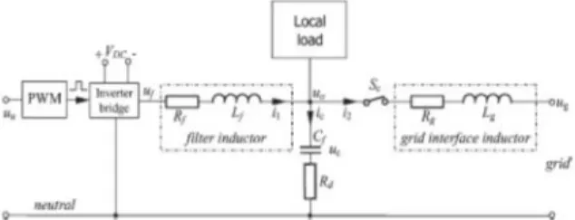
Fig. 1 shows the arrangement of a single-phase inverter connected to the grid. It consists of an inverter bridge, an LC filter, and a grid interface inductor connected with a circuit breaker. It is worth noting that the local loads are connected in parallel with the filter capacitor.
Fig. 1. Sketch of a grid-connected single-phase inverter with local loads
The current i1 flowing through the filter inductor is called the filter inductor current in this paper, and the current i2 flowing through the grid interface inductor is called the grid current in this paper. The control objective is to maintain low THD for the inverter local load voltage uo and
Fig. 2. Control plant Pufor the inner voltage
controller.
Fig. 3. Control plant Pifor the outer current
controller.
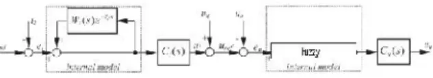
As a matter of fact, the system can be regarded as two parts, as shown in Figs. 2 and 3, cascaded together. For this reason, a cascaded controller can be adopted and designed. The proposed controller, as shown in Fig. 4, consists of two loops: an inner voltage loop to adjust the inverter local load voltage uo and an outer current loop to
adjust the grid current i2. According to the basic principles of control theory about cascaded control, if the dynamics of the outer loop is designed to be slower than that of the inner loop, then the two loops can be designed separately. Consequently, the outer-loop controller can be designed under the assumption that the inner loop is already in the steady state, i.e., uo = uref . It is also worth stressing that the current controller is in the outer loop and the voltage controller is in the inner loop.
Fig. 4. Proposed cascaded current–voltage controller for inverters, where both controllers adopt the H∞
repetitive and fuzzy strategy.
This is divergent to what is normally done. In this paper, both controllers are designed using fuzzy and H∞repetitive control strategy because of its outstanding performance in reducing THD. The voltage controller main objectives are the following: to deal with power quality problems of the inverter local load voltage even under unbalanced and/or
nonlinear local loads, to generate and dispatch power to the local load, and to synchronize the inverter with the grid. Whenever the inverter is synchronized and connected with the grid, then the grid determines voltage and frequency ratings. The main purpose of the outer-loop current controller is to exchange a clean current with the grid even in the presence of grid voltage distortion and/or nonlinear (and/or unbalanced for three-phase applications) local loads connected to the inverter. The current controller can be used for over current protection, but usually, it is included in the drive circuits of the inverter bridge. A phase-locked loop (PLL) can be used to provide the phase information of the grid voltage, which is needed to generate the current reference Iref.
As the control arrangement described here uses just one inverter connected to the system and the inverter is assumed to be powered by a constant dc voltage source, no controller is needed to regulate the dc-link voltage (otherwise, a controller can be introduced to regulate the dc-link voltage). Another important feature is that the grid voltage ugis fed
forward and added to the output of the current controller. This is used as a synchronization method, and it does not affect the design of the controller, as will be seen later.
III. DESIGNING OF VOLTAGE CONTROLLER
The design of the voltage controller will be outlined hereinafter, following the detailed procedures proposed in [16]. An important feature different from what is known is that the control plant of the voltage controller is no longer the whole LCL filter but just the LC filter, as shown in Fig. 2. Lineal control theory uses mathematical models of a process and some specifications of the predictable behavior in close loop, to design a controller [9]. These control strategies are extremely used in systems that can be assumed as linear in certain range of their operation. Moreover, it is absolutely necessary to obtain a linear model that represents the relationship between input and output in order to design the controller [17].
Given the above points, linear control strategies could be restricted in design and performance. On the other hand, non-linear strategies such as Knowledge Based Fuzzy Control (KBFC) [10], outperform linear controllers in many of the cases exposed above. KBFC is based on human knowledge which adds several types of information and can mix different control strategies that cannot simply be added through an analytical control law. On top of that, like human knowledge, KBFC does not need an accurate mathematical model in order to work out a control action [9]. What is more, KBFC uses the experience and the knowledge of an expert about the behavior of the system in order to work out the control action.
A kind of KBFC is the rule-based fuzzy control, where the human knowledge is estimated by means of linguistic fuzzy rules in the form if then. Each rule describes the control action in a particular condition of the system. Control action that would be done by a human operator. Therefore, under a specific condition of the system (if condition1) can be specified an action (then action1).
A rule base could be defined throughout different conditions of a system in which each rule defines an action for a specific condition. In the same manner, both condition and action are represented by linguistic terms such as (large, medium, small) for condition and (increase a few, increase a lot) for actions, those linguistic terms belong to fuzzy sets with overlapped boundaries. Hence, by means of fuzzy sets it is possible to get smooth interpolation between different rules, in order to describe completely the behavior of the system with few rules. To represent the qualitative knowledge of a human expert fuzzy control can be implemented based on that characteristic.
Fig.5 Membership functions
The controllers are based on a Mamdani fuzzy inference system, that kind of controllers are usually used into feedback systems because the rule base represents a static mapping between antecedents and consequents
Table: Rule table
∆e/e NB NS ZE PS PB
NBC BD MD SD SD NC
NSC MD SD NC NC SI
NC SD SD NC SI SI
PSC SD NC NC SI MI
PBC NC SI SI MI BI
IV. DESIGNING OF CURRENT CONTROLLER
As mentioned before, when designing the outer-loop current controller, it can be understood that the inner voltage loop tracks the reference voltage perfectly, i.e., uo = uref . Hence, the control plant for the current loop is simply the grid inductor, as shown in Fig. 3. The formulation of the H∞ control problem to design the H∞compensator Ciis
similar to that in the case of the voltage control loop shown in Fig. 5 but with a different plant Piand the
subscript u replaced with i.
A. State-Space Model of the Plant Pi
Since it can be assumed that uo= uref, there is uo= ug+ uior ui= uo−ugfrom Figs. 3 and 4, i.e.,
ui is actually the voltage dropped on the grid inductor. The feed forwarded grid voltage ug provides a base local load voltage for the inverter. The same voltage ugappears on both sides of the grid
interface inductor Lg, and it does not have an effect
on the controller design. Therefore, the feed forwarded voltage path can be ignored during the design process.
TABLE I
PARAMETERS OF INVERTER
Parameter Value Parameter Value
Lf 150µH Rf 0.045Ω
Lg 450µH Rg 0.135Ω
Cf 22µF Rd 1Ω
This is a very essential feature. The only contribution that needs to be careful during the design process is the output ui of the repetitive
current controller. The grid current i2flowing through the grid interface inductor Lg is chosen as the state variable xi= i2. The external input is wi= iref, and the control input is ui. The output signal from the plant Pi
is the tracking error ei= iref− i2, i.e., the difference between the current reference and the grid current. The plant Pi can then be described by the state
equation as follows:
and the output equation
= = + +
where
= − = 0 =
= −1 = 1 = 0
The corresponding transfer function of Piis
= .
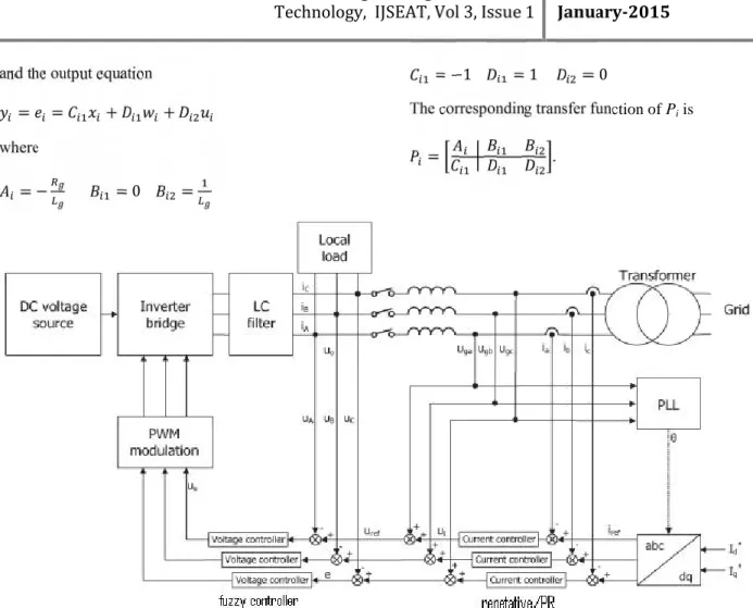
Fig. 6. Sketch of a grid-connected three-phase inverter using the proposed strategy.
B. Formulation of the Standard H∞Problem
Similarly, a standard H∞ problem can be formulated as in the case of the voltage controller shown in Fig. 5, replacing the subscript u with i. The resulting generalized plant can be obtained as
=
⎣ ⎢ ⎢ ⎢ ⎡
0 0
0 0
0
0 0 μ
⎦ ⎥ ⎥ ⎥ ⎤
(6)
with weighting parameters ξi and μi and low-pass
filter
=
, which can be selectedsimilarly as the corresponding ones for the voltage controller. The controller Ci can then be found
according to the generalized plant˜Piusing the H∞
control theory, e.g., by using the function hinfsyn provided in MATLAB.
C. Design of the H∞Current Controller
According to [16] and [18], the filter Wiwas chosen
= −2555 25501 1 and the weighting parameters were chosen as ξi = 100 and μi = 1.8. The H∞
controller Ciwhich nearly minimizes the H∞norm of
the transfer matrix from ˜ wi to˜ziwas obtained by
using the MATLAB function hinfsyn as
( ) =( . ×. )(( )).
The factor s + 4.334 × 10⁸ in the denominator can be approximated with the constant 4.334 × 10⁸ without causing any perceptible performance change. The resulting reduced controller is
( ) = . ( ).
The above-designed controller was implemented to estimate its performance in both stand-alone and grid connected modes with different loads. The faultless transfer of the operation modes was also carried out. The H∞ repetitive current controller was replaced with a proportional–resonant (PR) current controller for comparison in the grid-connected mode. In the stand-alone mode, in view of the fact that the grid current reference was set to zero and the circuit breaker was turned off (which means that the current controller was not functioning), the simulation results with both the repetitive current controller and the PR current controller are analogous, and hence, no comparative results are provided for the stand-alone mode. The PR controller was designed with the plant used as
( ) = 0.735 + .
A. In the Stand-Alone Mode
The voltage reference was situate to the grid voltage (the inverter is synchronized and ready to be connected to the utility grid). The assessment of the proposed controller was made for a resistive load (RA
= RB = RC = 12 Ω), a nonlinear load (a three-phase
uncontrolled rectifier loaded with an LC filter with L = 150μH and C = 1000μF and a resistor R= 20 Ω), and an unbalanced load (RA= RC= 12 Ωand RB=∞).
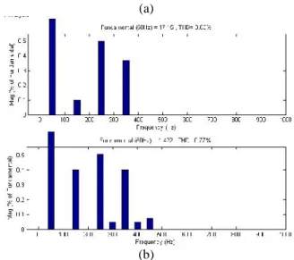
1) With the Resistive Load: The local load voltage uA,
voltage reference uref, and filter inductor current iA
are shown in Fig. 7(a). And then Fig. 7(b) shows the spectrum of the inverter local load voltage and the local load current. The recorded local voltage THD was 0.63%, while the grid voltage THD was 0.89%. In view of the fact that the utility grid voltage was used as the reference, it is worth mentioning that the excellence of the inverter local load voltage was better than that of the grid voltage, even without using an active filter.
(a)
(b)
Fig. 7. Stand-alone mode with a resistive load. (a) (Upper) uAand its reference urefand (lower) current
iA. (b) (Upper) Voltage THD and (lower) current
THD.
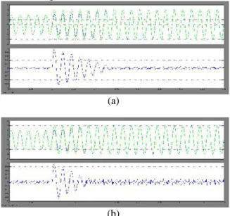
2) With the Nonlinear Load: The local load voltage uA, voltage reference uref, and filter inductor current iAare shown in Fig. 8(a). The spectra of the inverter
local load voltage and the local load current are shown in Fig. 8(b). The recorded local load voltage THD was 2.27%, while the grid voltage THD was 1.78%. The simulation results make obvious acceptable performance of the voltage controller for nonlinear loads.
3) With the Unbalanced Load: The inverter local load voltage and the local load currents are shown in Fig. 9(a) with their spectra shown in Fig. 9(b). The recorded local load voltage THD was 0.68%, while the grid voltage THD was 0.50%.
(b)
Fig. 8. Stand-alone mode with a nonlinear load. (a) (Upper) uAand its reference urefand (lower) current
iA. (b) (Upper) Voltage THD and (lower) current
THD.
In view of the fact that the proposed control structure adopts separate controllers for each phase, the unbalanced loads had no influence on the voltage controller performance, and the inverter local load voltages remain balanced.
B. In the Grid-Connected Mode
The current reference of the grid current I*d
was set at 2 A (corresponding to 1.41 A rms), after connecting the inverter to the grid. And the reactive power was set at 0 var (I*q = 0). The resistive, nonlinear, and unbalanced loads used in the previous section were used once again. Furthermore, the case without a local load was carried out as well. At last, the transient responses of the system were evaluated.
(a)
(b)
Fig. 9. Stand-alone mode with an unbalanced load. (a) (Upper) Inverter local load voltage and (lower) local load currents. (b) (Upper) Voltage THD and
(lower) current THD.
1) Without a Local Load: The spectra of the inverter local load voltage and the grid current of both controllers are shown in the left column of Fig. 10. The recorded THD of the local voltage was 0.51% for the proposed controller and 0.51% for the PR controller, while the grid voltage THDs were 0.51% and 0.51%, respectively. The THD of the grid current was 1.38% for the proposed controller and 2.73% for the PR controller. In this simulation, the proposed controller outperforms the PR-current–fuzzy voltage controller. Note that the grid was cleaner when the PR-current- fuzzy based voltage controller was tested.
2) With the Resistive Load: The spectra of the inverter local load voltages and grid currents are observed in the middle-left column of Fig. 10. When the resistive local load is connected, the recorded local load voltage THD was 0.60% for the proposed H∞controller and 0.47% for the PR controller, while the grid voltage THDs were 0.60% and 0.47%, respectively. The grid current THD was 1.19% for the proposed H∞ controller and 2.58% for the PR controller. The presentation of both controllers remains almost unchanged with comparison to the previous simulation without a local load. The proposed controller again outperforms the PR current– fuzzy-voltage controller. Observe that the grid was cleaner again when the PR-current-fuzzy-voltage controller was tested.
4) With the Unbalanced Load: The spectra of the inverter local load voltage and the grid current are exposed in the right column of Fig. 10. The recorded local load voltage THD was 0.53% in the case with the H∞current controller and 0.49% in the case with the PR controller, while the grid voltage THDs were 0.53% and 0.49%, respectively. The grid current THDs were 1.20% and 2.54%, respectively. Both schemes can inject balanced clean currents to the grid even though the local load is not balanced.
C. Transient Performance
1) Transient Response to the Change of the Grid Current Reference (No Local Load Connected): A step change in the grid current I∗dreference from 2 A
(1.41 A rms) to 3 A (2.12 A rms) was applied (while
keeping I∗q= 0). The grid current ia, its reference iref, and the current tracking error eiare shown in Fig. 11.
The proposed controller took about 12 cycles to settle down, and the PR-current–fuzzy based voltage controller took about eight cycles to settle down. This is reasonable because each repetitive controller takes about five cycles to settle down. This reflects the exchange between low THD and system response speed.
2) Transient Response to the Change of the Resistive Local Load: The filter inductor current and the grid current, jointly with the reference current and the tracking error, when the three-phase resistive local load was changed from RA= RB= RC= 12 Ω to RA=
RB= RC= 100 Ωand back, are shown in Fig. 12.
(a)
(b)
Fig. 10. Spectra of the inverter local load voltage and the grid current with (left column) no load, resistive load (middle-left column), (middle-right column) nonlinear load, and (right column) unbalanced load. (a) H∞repetitive
D. Seamless Transfer of the Operation Mode
The transient response of the grid current when the inverter was changed it’s mode from the stand-alone to the grid connected mode and back is shown in Fig. 13.
(a)
(b)
Fig. 11. Transient response in the grid-connected mode without local load to 1-A step change in I*d:
(Upper) Grid current iaand its reference irefand (lower) current tracking error ei. (a) H∞repetitive
current–fuzzy based voltage controller. (b) PR-current-fuzzy based voltage controller.
Fig. 12. Transient responses of the inverter and grid currents when the local load was changed. Filter
inductor current iA. (upper) Grid current ia, its
reference iref(middle) , and the current tracking error ei(lower).
Fig. 13. Transient response of the inverter when transferred from the standalone mode to the
grid-connected mode and then back.
VI. CONCLUSION
Hence in micro grids the cascaded current-voltage control strategy has been proposed for inverters to improve the power quality. This scheme consists of an inner voltage loop and an outer current loop and offers excellent performance in terms of THD for both the inverter local load voltage and the grid current. Especially, when nonlinear and/or unbalanced loads are linked to the inverter in the grid-connected mode, the proposed scheme extensively improves the THD of the inverter local load voltage and the grid current at the same time. The controllers are designed using the H∞repetitive current control and fuzzy based voltage control in this paper. The proposed approach also achieves faultless transfer between the stand-alone and the grid-connected modes. The approach can be used for single-phase systems or three-phase systems. Therefore, the nonlinear harmonic currents and unbalanced local load currents are all contained locally and do not have an effect on the grid. Simulation results under various scenarios have demonstrated the excellent performance of the proposed scheme.
REFERENCES
[1] N. Hatziargyriou, H. Asano, R. Iravani, and C. Marnay, “Microgrids,” IEEE Power Energy Mag., vol. 5, no. 4, pp. 78–94, Jul./Aug. 2007.
[2] F. Katiraei, R. Iravani, N. Hatziargyriou, and A. Dimeas, “Microgrids management,” IEEE Power Energy Mag., vol. 6, no. 3, pp. 54–65, May/Jun. 2008.
[3] C. Xiarnay, H. Asano, S. Papathanassiou, and G. Strbac, “Policymaking for microgrids,” IEEE Power Energy Mag., vol. 6, no. 3, pp. 66–77, May/Jun. 2008.
[4] Y. Mohamed and E. El-Saadany, “Adaptive decentralized droop controller to preserve power sharing stability of paralleled inverters in distributed generation microgrids,” IEEE Trans. Power Electron., vol. 23, no. 6, pp. 2806–2816, Nov. 2008. [5] Y. Li and C.-N. Kao, “An accurate power control strategy for powerelectronics- interfaced distributed generation units operating in a lowvoltagemultibus microgrid,” IEEE Trans. Power Electron., vol. 24, no. 12, pp. 2977–2988, Dec. 2009.
mode transfer microgrid applications,” IEEE Trans. Power Electron., vol. 25, no. 1, pp. 6–15, Jan. 2010. [7] J. Guerrero, J. Vasquez, J. Matas, M. Castilla, and L. de Vicuna, “Control strategy for flexible microgrid based on parallel line-interactive UPS systems,” IEEE Trans. Ind. Electron., vol. 56, no. 3, pp. 726– 736, Mar. 2009.
[8] Z. Yao, L. Xiao, and Y. Yan, “Seamless transfer of single-phase gridinteractive inverters between grid-connected and stand-alone modes,”IEEE Trans. Power Electron., vol. 25, no. 6, pp. 1597–1603, Jun. 2010.
[9] Q.-C. Zhong and G. Weiss, “Synchronverters: Inverters that mimic synchronous generators,” IEEE Trans. Ind. Electron., vol. 58, no. 4, pp. 1259–1267, Apr. 2011.
[10] Q.-C. Zhong, “Robust droop controller for accurate proportional load sharing among inverters operated in parallel,”IEEE Trans. Ind. Electron., vol. 60, no. 4, pp. 1281–1290, Apr. 2013.
[11] M. Prodanovic and T. Green, “High-quality power generation through distributed control of a power parkmicrogrid,” IEEE Trans. Ind. Electron., vol. 53, no. 5, pp. 1471–1482, Oct. 2006.
[12] Y. W. Li, D. Vilathgamuwa, and P. C. Loh, “A grid-interfacing power quality compensator for three-phase three-wire microgrid applications,” IEEE Trans. Power Electron., vol. 21, no. 4, pp. 1021– 1031, Jul. 2006.
[13] D. Vilathgamuwa, P. C. Loh, and Y. Li, “Protection of microgrids during utility voltage sags,” IEEE Trans. Ind. Electron., vol. 53, no. 5, pp. 1427– 1436, Oct. 2006.
[14] F. Blaabjerg, R. Teodorescu, M. Liserre, and A. Timbus, “Overview of control and grid synchronization for distributed power generation systems,”IEEE Trans. Ind. Electron., vol. 53, no. 5, pp. 1398–1409, Oct. 2006.
[15] G.Weiss, Q.-C. Zhong, T. Green, and J. Liang, “H∞ repetitive control of DC–AC converters in micro-grids,” IEEE Trans. Power Electron., vol. 19, no. 1, pp. 219–230, Jan. 2004.
[16] T. Hornik and Q.-C. Zhong, “H∞ repetitive voltage control of gridconnected inverters with frequency adaptive mechanism,” IET Proc. Power Electron., vol. 3, no. 6, pp. 925–935, Nov. 2010. [17] T. Hornik and Q.-C. Zhong, “H∞ repetitive current controller for gridconnected inverters,” in Proc. 35th IEEE IECON, 2009, pp. 554–559.
[18] T. Hornik and Q.-C. Zhong, “A current control strategy for voltage-source inverters in microgrids based onH∞ and repetitive control,” IEEE Trans. Power Electron., vol. 26, no. 3, pp. 943–952, Mar. 2011.
AUTHOR’S PROFILE
VISHNU VARDHAN
REDDY was born in
sunkesula village, Khajipet mandal, kadapa district, Andhra Pradesh, INDIA. He received his B.Tech degree (Electrical and Electronics Engineering) from the Mekapati Rajamohan Reddy Institute of Technology & Science, Udayagiri, Nellore district in 2009 and pursuing M.Tech (Power Systems) from the Global College of Engineering & Technology, Kadapa.
Mrs. M Rama Subbamma