Core Module Optimizing PDE Sparse Matrix Models with
HPCG Example
Earle Jennings1
c
The Author 2017. This paper is published with open access at SuperFri.org
This paper introduces a fundamentally new computer architecture for supercomputers. The core module is application compatible with an existing superscalar microprocessor, with minimized energy use, and is optimized for local sparse matrix operations. Optimized sparse matrix manip-ulation is discussed by analyzing the High Performance Conjugate Gradient (HPCG) benchmark specification. This analysis shows how the DRAM memory wall is removed for this benchmark, and for sparse matrix models of partial differential equations (PDEs) for a wide cross section of applications. By giving the programmer improved control over the configuration of the super-computer, the potential for communication problems is minimized. Application compatibility is achieved while removing the superscalar instruction interpreter and multi-thread controller from the existing microprocessor’s hardware. These are transformed into compile-time utilities. The instruction cache is removed through an innovation in VLIW instruction processing. The data caches are unnecessary and are turned off in order to optimally implement sparse matrix models. Keywords: HPCG, superscalar, sparse matrix, partial differential equation, memory wall, HPC.
Introduction
Today’s high performance, superscalar microprocessor includes a superscalar instruction in-terpreter [12], instuction and data caches, as well as a multi-thread controller [19]. These elements consume more than 90% of the silicon and more than 90% of the energy, without processing any of the data. These are the energy monsters in today’s high performance microprocessors. This paper introduces a core module known as the Simultaneous Multi-Processor (SiMulPro) core module, which removes all of these problems.
Application Compatibility
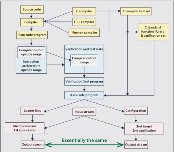
Application compatibility requires the existing compiler technology remain basically un-touched. Removing the hardware overhead of the superscalar instruction interpreter, multi-thread controller and the instruction cache, requires that the SiMulPro core module be seman-tically compatible with the existing microprocessor of Figure 1. This means that each assembly language program needs to generate two applications, the first for the microprocessor, which is the first target of existing software tools. The second target is the SiMulPro core module, which does not implement the microprocessor’s Instruction Set Architecture (ISA). This is discussed in section 1. Semantic compatibility is established for this assembly language program when both applications respond to the same input stream by generating essentially equal output streams.
Confirming application compatibility needs to be cost effectively managed by breaking this job into several steps. For High Performance Computers (HPC), particularly supercomputers, C, C++ and Fortran compilers are the most commonly used. Consider the C compiler. It has a compiler test set, which is used today to confirm generated assembly code targeting the microprocessor. The first step of verifying application compatibility uses this C compiler test set to verify semantic compatibility with the second target (SiMulPro core and core module) from its generated assembly language programs. The compiler test set is exercised through the C
compiler to generate its family of assembly test programs. These generated assembly programs can verify semantic compatibility, and therefore application compatibility, between the existing microprocessor and the SiMulPro core module.
A second step uses the assembly code programs of one, or more, C function libraries, each with their verification set, to extend verification of semantic compatibility between these two targets. At this point, there are two ways to proceed. One approach continues to the C++ and Fortran compilers, their test sets, and so on. The other approach starts from the compiler output opcode range, and successively extends testing, using the verification and test suite of the microprocessor. The verification can extend beyond the compiler output opcode range, to include more, possibly all, of the ISA.
Figure 1. Semantic compatibility confirmed against both compiler technology and the verifica-tion and test set of the microprocessor implementing an Instrucverifica-tion Set Architecture (ISA)
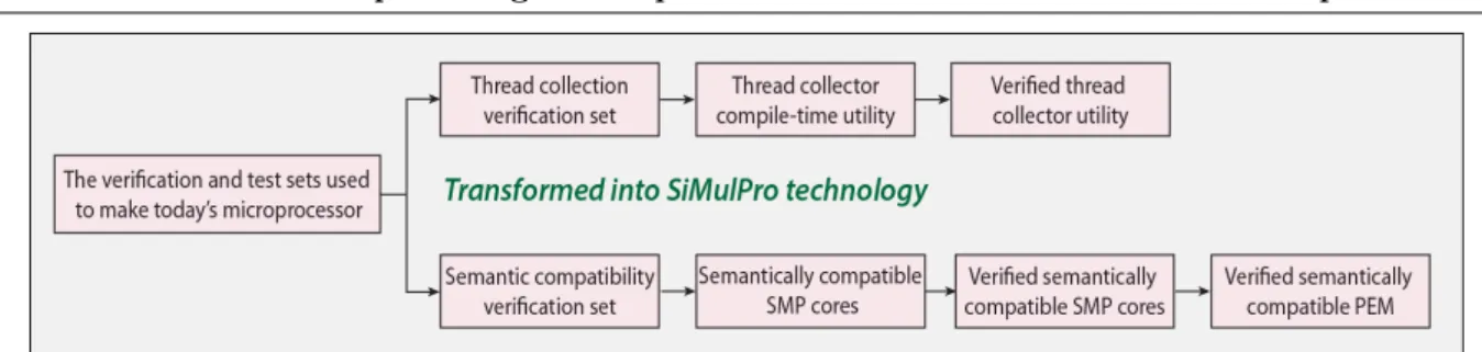
Figure 2.Components of the verification and test set and of the generated SiMulPro technology
1. Simultaneous Multi-Processor (SiMulPro) Cores And Core
Module
This simple SiMulPro core supports two simultaneous processes. It implements a simulta-neous process state calculator, which issues two process states for executing these processes.
Figure 3. A simple SiMulPro core
Each of these simultaneous processes separately owns instructed resources. The separated ownership means that both processes cannot contend for the same resource, making them im-mune to stalling from contentions. Each instructed resource includes its own local instruction processor, which can access its own local instruction memory component. The state of each process stimulates each owned, local instruction processor. Each instruction processor accesses its own local instruction memory to generate the local instruction to direct that resource. Each of the processors includes its simultaneous process and its owned resources.
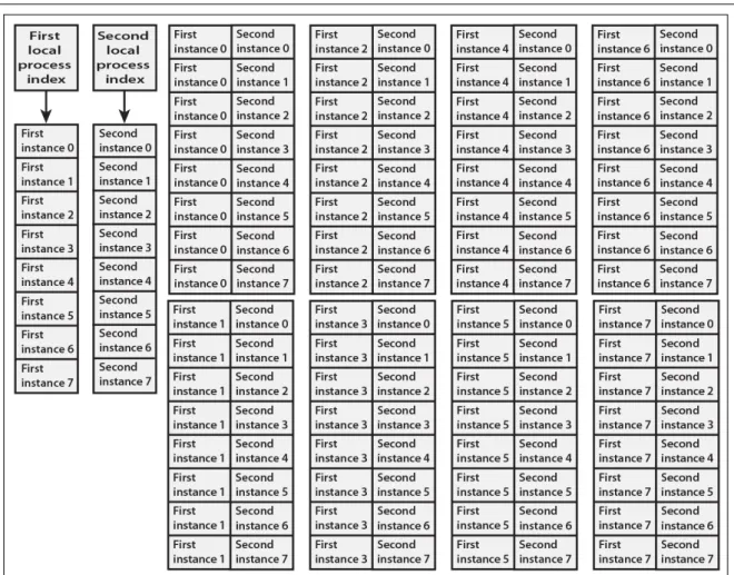
Figure 4 shows a use of this simplified SiMulPro core. The right hand side is characteristic of the Multiflow [6], and the EPIC architecture [16], which led to the I-64 [11] and the Itanium [17]. The Mill computer [7] bears some resemblance to the left hand side, but has only two instruction pointers.
Figure 4.The first and second SiMulPro processes each have 8 process states, shown on the left. A single VLIW instruction pointer requires an equivalent VLIW memory of 64 VLIW words, shown on the right
instruction caching. Also, all predecessor VLIW approaches require unique compilers, which negates application compatibility.
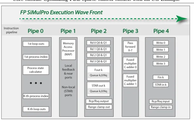
Figure 5 shows the FP SiMulPro core including the process state calculator, which generates multiple process states (or indexes) and their corresponding loop outputs, on every clock cycle. This is shown in instruction pipe 0. These process states, etc., form an execution wave front, which successively traverses each instruction pipe. Assume each instructed resource includes 256 local instructions per task. If K is 4, this is a virtual VLIW instruction space of 4 Giga-VLIW instructions. If K is 6, this is 256 Tera-VLIW instructions.
Pipe 1 includes the Memory Access Processor (MAP), which generates all local addressing for many standard access patterns, including matrix and vectors, buffering, and FFTs. During local, linear algebra operations, as in Linpack, all non-floating point cores are turned off. The system capabilities of instruction pipes 2 and 4 are coupled:
Figure 5.Example FP SiMulPro core supporting K simultaneous processors
• Data is fed back from instruction pipe 4 to output queues in instruction pipe 2. This feed mechanism also provides a router-less feed interface to neighboring modules. This is more energy efficient, because hardware routers are not needed.
• Farther communication uses the STAR (Simultaneous Transmit And Receive) input port of pipe 4 and output queues of pipe 2. The transfer request channel sends to a memory controller the parameters for each programmed memory access pattern. The state of the core modules can be saved with an acceptable overhead. The memory controllers can re-spond to anticipating memory requests, which preload data into the controller for low latency transfers when the data is actually needed. This combined with the VLIW in-struction space makes caches unnecessary. Each channel can transmit and receive a STAR message on each local clock cycle, assumed to be 1 ns. The application layer of the STAR message includes a package with a payload of 128 + 5 bits and a context field of 32 bits. The payload can hold two double precision numbers, sufficient to efficiently download, or upload, the state of the cores in a Data Processing Chip (DPC). Also, the payload can hold a double precision number and an index list, which can represent a non-zero entry in a sparse matrix, or a vector component associated with one, or more, of the non-zero, sparse matrix entries. This package with, or without the context, is supported by the arithmetic and feed interfaces as well, so that sparse matrix processing, as well as matrix pivots, are consistently and efficiently supported.
• Reciprocals, reciprocal square roots and a range clamp circuit, for range limiting of tran-scendental functions, are each supported with input in pipe 4 and output in pipe 2.
algorithms can go from coarse (16 bit), to finer, and finest arithmetic (64 bit posit), with re-duced communication overhead, and memory access for early iterations. Neural networks and deep learning can operate in 16 bit mode, providing 8 posit multiply-accumulates per execution wave front.
Within each execution wave front, a use vector, of the used resources is generated. Within the wave front, a use bit drives a power gate generating a gated power used by the resource, for each resource. In CMOS, the clock may be gated to control power. However, in technologies such as memristors and molecular gates, other specific mechanisms may provide this capability.
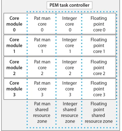
2. Core Modules And Programmable Execution Module (PEM)
Figure 6. The PEM contains 4 core modules, each including 3 types of SiMulPro cores
The PEM is roughly a quad core superscalar microprocessor, without the overhead. Note that without this overhead Data Processor Chips (DPCs) can scale from about 60 core micropro-cessors to ten times that many core modules, with about the same power and silicon as today’s chips. Instances of the same typed cores, such as the FP cores discussed above, can share their instructed resources. This increases the virtual VLIW space. Assume each FP core supports 6 simultaneous processors and 256 instructions per resource. The VLIW instruction space is then 2(4∗6∗8)= 2192= 222(19∗10)>4∗1057.
DRAM. This saves at least 15% of the energy used in the core module. Pat Man organizes and directs the FP and integer activities needed for local sparse matrix operations.
Each core module can operate as a seperate unit. Core module 0 may perform a simulation of one object. Simultaneously, core module 1 may simulate a second model. Alternatively, each core module may be configured to model the same object, but at differing geometric locations.
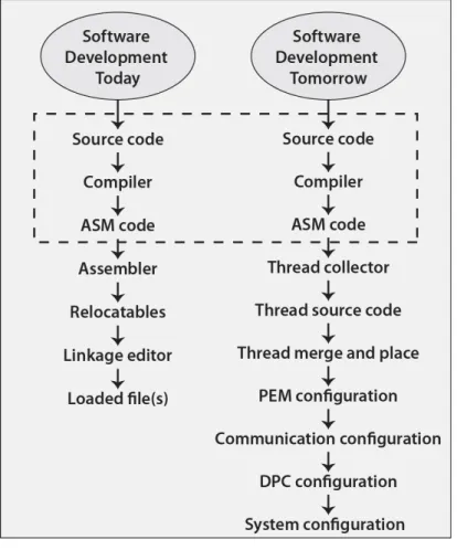
3. Software Development Today And Tomorrow
The compiler is basically unchanged between today and tomorrow. The superscalar inter-preter hardware, in particular its behavioral model, is transformed into the thread collector utility as shown in Figures 2 and 6. The thread collector is now a compile-time utility receiving assembly code, which it translates into microcode. The microcode is then scheduled, as close to the start of a thread as allowed by the preceding assembler instructions. The thread collector outputs these sequenced micro code instructions as one, or more, thread source code files.
Figure 7. Software Development Summary
behav-ioral models of the microprocessor’s data processing resources are injected into SiMulPro core templates to create the core module. The semantic compatibility verification set is derived, as discussed above, from the compiler test sets, etc.. Exercising the core model with the semantic compatibility verification set generates the verified, semantically compatible SiMulPro cores and core module. Verifying the core module creates the semantically compatible PEM.
3.1. Threads
Today, a thread of execution, is the smallest sequence of program instructions which can be managed independently by a scheduler in an operating system. In this architecture, threads are operations of at least one core, in a PEM, expressed as one or more processes. Consider the following example shown in Figure 8 of a process defined in a thread source code file.
process DotAccum // Declarations FeedbackInput
ProductIn 1, DotAccum 2; FeedbackOut
ProductFedback1 ProductIn 1; DotFedback[1:5] DotAccum[1:5]; C-Adder DotAccum 0; STAR Out Data DotOut 0; // Process List
ProcessStates
DPaccum6, // highest priority, least probable process state DPaccum5, DPaccum4, DPaccum3, DPaccum2, DPaccum1,
DPaccum0; // least priority and most probable state endProcessStates;
Endprocess;
Figure 8. Short example of thread source code
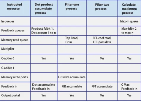
After collecting the threads, the intermediate program representation is analyzed from the thread source code files, and thread merging begins. Consider the following example of processes shown in Figure 9, all to be placed in the same core after merging. Note that these four processes share ownership of C-adder0, as they all use this resource. Consider how actions are triggered by a simultaneous process. Each process owns all of its stimulators, which can be queues associated with one or more RAM read ports, feedback, feed local or feed farther (STAR) sources. The process can also be stimulated by the state of internal loop registers. Assume that the four processes of Figure 9 are to be merged and have the following process states:
Table 1.The states of the processes to be merged
Dot Accum Filter 1 Filter 2 Max Calc Merged
DPaccum6 Facc2 F2acc3 Max5 DPaccum5 Facc1 F2acc2 Max4 DPaccum4 Facc0 F2acc1 Max3 DPaccum3 F2acc0 Max2
DPaccum2 Max1
DPaccum1 Max0
DPaccum0
Given that the highest priority state of each process (shown in the top row) is its least probable state, merging there processes proceeds by first listing the highest priority states of each process as shown in the Merged 1 column:
Table 2.Resulting top states of the merged process
Dot Accum Filter 1 Filter 2 Max Calc Merged 1 Merged 2
DPaccum6 Facc2 F2acc3 Max5 DPaccum6 DPaccum6 DPaccum5 Facc1 F2acc2 Max4 Facc2 Facc2 DPaccum4 Facc0 F2acc1 Max3 F2acc3 F2acc3 DPaccum3 F2acc0 Max2 Max5 Max5
DPaccum2 Max1 DPaccum5
DPaccum1 Max0 Facc1
DPaccum0 F2acc2
The merging of these processes continues in this fashion as shown in the Merged 2 column. At runtime, the instruction set operations are gone, replaced by their microcode sequences, sched-uled as opportunistically as the assembly program segment permits, and then, possibly, merged with other simultaneous processes. This runtime situation is new to application developers. They need to know what processes have been initiated.
Table 3.Example of a thread condition register
Thread Condition Register Collapse Cond Cond Cond Cond
Count 0 1 ... p
it releases its processes to respond to feedback, input and loop conditions. For instance, each thread may use a 2 bit arithmetic condition code, where ’00’ means == 0, ’01’ means >0, ’10’ means <0, and ’11’ means unavailable. Arithmetic error codes may be represented by another 2 bit code, where ’00’ means normal, ’01’ means infinite generated, ’10’ means Not A Number (NAN) generated, and ’11’ means unavailable.
subprogram X1(parm list) {
code 1 // cond state length = 0 Cond collapse = 0
if test1 // 0 0
{ code 2) // 1 0
else { code 3 // 2 0
} code 4 // 1 1
}
Figure 10.Example showing condition length and collapse count of the condition code register
Let’s look briefly at what is needed to aid the programmer in this post-branching architec-ture. We need a semantic content that consistently describes branching across Fortran, C and C++, at a minimum. Let’s focus on Arithmetic IFs from Fortran, the switch conditional from C, and Range limiting for transcendental functions. Each of these branching mechnisms can be described by 2 bit encoding of trinary condition states, making it a feasible and consistent choice across all three languages. We also need some form of loop constructs that account for the looping of these languages. Fortunately, C provides us with two primitives into which the other implementations can be mapped:
do { body1 } while test1; while test2 do { body2 };
Figure 11.Thread Placement for Block LU Decomposition in one Data Processor Chip
distinct threads. However, each core, in each of the PEM, can be configured differently. Complex parsers, data analytics, numerically intensive, and all other manner of threads, can be placed to create networks of state machines. These networks can be unique to each DPC. These state machine networks optimize the big computational, and the big data, processing of tomorrow.
4. Introduction To Sparse Matrix Mathematics And Models
A matrix is a 2-D rectangular array of numbers, either FP or posit numbers. A sparse matrix
A= [ai,j] is a matrix in which most numbers are zeros. A column vectorx=
h
x0 ... xN
iT
is called a stimulus and a vector b = h b0 ... bN
iT
is called a response when Ax = b, or
X
ai,jxj =bi for all i.
Matrix mathematics [8] is an innately useful tool in many applications [14]. In particular, sparse matrix math [15] has been harnessed to approximate solutions to partial differential equations [1], [18] specifically, 3-D models of physical systems, which includes fluids, stress and strain of solids, the dynamics of molecules, plasmas [2], as well as the weather.
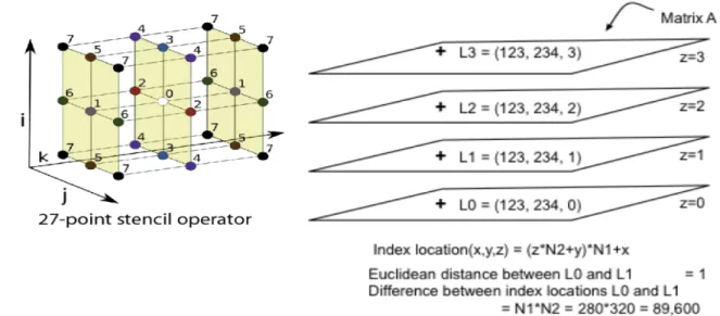
Many differential operators, for example the Laplacian, support very stable and efficient finite difference approximations, such as the 27 stencil model [13] used in HPCG benchmark [10].
Figure 12. On left is the 27 point stencil from the HPCG specification, and on right, the index enumeration problem for finite difference schemes
These fetches of the stimulus vector are likely to trigger cache faults. To execute these sparse linear models efficiently, we need to situate the geometric neighborhoods of the model system in a single core. By concentrating the relevant geometric information in one core, data caching is unneeded. The main memory is accessed only once, eliminating the memory wall problem.
5. Local Implementation Of Sparse Matrix Solvers For A
Geometric Neighborhood
The indexing rasterization discussed above for the 3-D model of HPCG, leads to an index location calculated as
IndexLocation x, y, z = (z∗N2 +y)∗N1 +x=IL
implying a localization function, which generates x, y, and z by performing
k=f loor(IL/N1)
x=rem(IL/N1)
y=rem(k/N2)
z=f loor(k/N2)
Note that HPCG sets N1 = 280 andN2 = 320.
Figure 13.Allocation of FP RAM in Vector stores with the indexing mirrored by Int RAM
locally. The response vector components correspond to one of the row indexes of the matrix rows being stored locally. The vector length is chosen so that the stencil can be stored in just one vector store, and the boundary stencils fit naturally within this vector store, without requiring garbage collection. The integer RAM contains the indexes of the corresponding FP RAM locations. The Pat Man core keeps track of the management tables for the FP and Int Cores. Note that in some implementations the vector stores for the stimulus and response vectors may be organized differently.
6. Introduction To The Pat Man Core
Figure 14.Block diagram of the Pat Man core
The Pat Man core shown in Figure 14 is a SiMulPro core, with the following components.
1. The C1-adders of pipe 3 match the index list of a received package to determine which global object is being referenced, whether the package should be stored in this core module, and whether the global object uses finite difference, or finite element, indexing. Often, finite element indexing is organized to reveal geometric proximity.
2. Divmod in and Divmod out of pipes 4 and 2, respectively implement various schemes for 2-D, 3-D (shown above) index location conversion to geometric address. Higher dimensional indexing may also be supported.
3. Pattern Recognizers (PatRecs) use either the index list (for finite element indexing), or the derived geometric addresses, to determine which vector store holds the package numeric data.
or more, of the communication mechanisms. The received vector updates are used by the Pat Man cores to update the readiness of the local sparse rows for processing. When a row is ready for processing, the PatMan sends a message to the FP and Int cores, which is queued until the cores are ready to begin those operations.
7. Basic Systems Analysis Of Sparse Matrix Performance
While HPCG is not a real program solving one or more partial differential equations, several things can be done to evaluate what will happen to other application models of similar size. Each of the FP RAM includes 4K words, which supports 151 vector stores. If 25% of these stores are allocated to the local components of the vectors, each core module can execute about 110 rows of the sparse matrix. The 48,384,000 rows of HPCG, and comparable models, fit in 440K core modules, or about 764 Data Processor Chips (DPCs), which each contain 144 PEM, or 576 core modules. Assuming 16 DPC chip stacks per optical PCB and 12 PCB’s per optical motherboard, this is essentially a single rack containing 4 optical motherboards. This rack, once loaded from the DRAM, never needs to access the DRAM for the matrix values, or vector values, until the run is over, or the DRAM needs updating due to adaptive grid generation, or refinements of the finite element cells (etc.).
The remaining overhead is primarily the communication overhead for vector updates. Con-sider a worst case situation for HPC. Suppose a tokamak reactor containing plasma is simulated as the interior of a torus as shown in Figure 15. This is a very simplified discussion, which will not require detailed knowledge of plasma physics nor the specifics of a particular solution algo-rithm for such equation systems. Simply assume this model saturates a supercomputer covering a computer floor of roughly 40 meters on a side. Further assume the torus is modeled as a sheet of core modules, which has its top and bottom edges (ab and cd) joined, then its left and right edges joined, which is a classic topological construction of the torus. This naive construction has just condemned the simulation to have a huge energy budget, as well as very poor communica-tion latency, because the body effect latency now includes the worst case propagacommunica-tion from the bottom left to the top right cabinets.
Figure 15.Making a torus by identifying sides, and then imposing a 2-D red-black ordering
cells meet the bottom cells within two neighboring PEM, and the worst case traversal path is just from one cabinet to an adjacent cabinet.
8. Summary
A fundamentally new computer architecture has been introduced. This architecture is ap-plication compatible with an existing superscalar microprocessor, which can be verified in a systematic, incremental approach lending itself to effective project management. The super-scalar instruction interpreter and multi-thread controller are removed from the microprocessor and transformed into compile-time utilities. Today’s compilers for the microprocessor are pre-served, essentially unaltered. The instruction cache is unneeded because of the huge, virtual VLIW space. Sparse matrix modeling of partial differential equations and HPCG, are optimized by removing the DRAM memory wall. Communication latency and throughput can be con-trolled by thread placement, as shown by the tokamak and block LU decomposition examples. New software tools, while maintaining today’s compilers, enable programs to be embodied by these supercomputers as algorithm state machine networks.
Energy use is minimized. The superscalar instruction interpreter, the caches, and the multi-thread controller are removed from hardware, giving at least a 10X reduction. Each SiMulPro core, gates off power to each unused resource on each clock. Local feed communications with neighboring PEM do not use routers. Sending access requests to external, anticipating memory controllers for DRAM, saves at least 15% of the energy used for memory address calculation. Sparse matrix solvers, in systems as small as a rack, are only loaded once from the DRAM.
I wish to thank Heather Murphree, John Gustafson, and George Pearson of MacKickan Software for their invaluable contributions. I wish to thank the reviewer for pointing to an in-consistency in the discussion of sparse matrices. Thanks to the HPCG team for their thinking and their excellent bibliography. Also, thanks to the applied mathematics community for giving us all such powerful tools for partial differential equations.
This paper is distributed under the terms of the Creative Commons Attribution-Non Com-mercial 3.0 License which permits non-comCom-mercial use, reproduction and distribution of the work without further permission provided the original work is properly cited.
References
1. Briggs, Henson, McCormick; A Multigrid Tutorial (2nd ed), DOI: 10.1137/1.9780898719505 (2000) Society of Industrial and Applied Mathematics (SIAM), Pihladelp[hia, PA, US
2. DOE; Scientific Grand Challenges in Fusion Energy Sciences and the Role of Computing at the Extreme Scale, https://science.energy.gov/~/media/ascr/pdf/
program-documents/docs/Fusion_report.pdf (2009) DOE, Office of Fusion Energy Sci-ences, Office of Advanced Scientific Computer Research March 18-20, 2009, US
3. DOE-ASCAC Subcommittee Report; Top Ten Exascale Research Challenges, science. energy.gov/~/media/ascr/ascac/pdf/meetings/20140210/Top10reportFEB14.pdf
4. Dongarra; Report on the Sunway TaihuLight System; (2016), University of Tennessee, Oak Ridge National Laboratory, Dept Electrical Engineering and Computer Science, Tech Re-port, UT-EECS-16-742, US
5. Ercegovac, Lang; Digital Arithmetic, https://www.elsevier.com/books/ digital-arithmetic/ercegovac/978-1-55860-798-9 Hardcover ISBN: 9781558607989 , (2003) Elsevier Sciences, San Franciso, CA, US
6. Fisher; Very Long Instruction Word Architectures and the ELI-512, https://doi.org/10.1145/800046.801649, (1983) ACM, US
7. Goddard; Ivan Goddard and Mill at the 2015 European LLVM Conference, April 14, 2015;
https://millcomputing.com/event/1725/
8. Golub, van Loan; Matrix Computations (4th ed); https://jhupbooks.press.jhu.edu/ content/matrix-computations-0ISBN: 9781421407944, (2013) Johns Hopkins University Press, Baltimore, Maryland, US
9. Gustafson; Beating Floating Point at its Own Game: Posit Arithmetic; http: //supercomputingfrontiers.com/2017/wp-content/uploads/2017/03/2_1100_
John-Gustafson.pdf (2017)
10. Heroux, Dongara, Luszcek; HPCG Technical Specification, SAND 203-8752,www.osti.gov/ scitech/biblio/1113870f(2013), Sandia National Labs, US
11. Huck, Morris, Ross, Kneis, Mulder, Zahir; Introducing the I-64 Architecture, http: //ieeexplore.ieee.org/document/877947/ (2000), IEEE Micro, Sept, 2000, pp 24-35, US
12. Johnson; Superscalar Microprocessor Design, https://books.google.com/books/about/ Superscalar_microprocessor_design.html?id=9o1TAAAAMAAJ (1991), Prentis Hall, En-glewood, NJ, US
13. O’Reilly; A Family of Large-Stencil Discrete Laplacian Approximations in Three Dimen-sions,ftp://grey.colorado.edu/pub/oreilly/misc/disc_lapl.3.pdf(2006) University of Colorado Boulder, CO, US
14. Press, Flannery, Teukolsky, Vetterling; Numerical Recipes in C: The Art of Scientific Pro-gramming 2nd ed.,http://apps.nrbook.com/c/index.html(1992) Cambridge University Press, Cambridge, England
15. Saad; Interative Methods for Sparse Linear Systems (2nd ed); DOI: 10.1137/1.97808987180 (2003) SIAM, Philadelphia, PA, US
16. Schlansker, Rau; EPIC: An Architecture for Instruction Level Parallel Processors, (Febru-ary 2000) www.hpl.hp.com/techreports/1999/HPL-1999-111.pdf HP Laboratories Palo Alto, HPL-1999-111
18. Trottenberg, Osterlee, Shueller, Stuben, Oswald, Brandt; Multigrid; https://books. google.com/books/about/Multigrid.html?id=9ysyNPZoR24C (2001) Academic Press, Harcourt Science and Technology Company, San Diego, CA, US
19. Ungerer, Robic, Silc; A Survey of Processors with Explicit Multi-Threading, http://www. academia.edu/26319932/A_survey_of_processors_with_explicit_multithreading