A General Guide to Applying Machine Learning to Computer
Architecture
Daniel Nemirovsky1, Tugberk Arkose1, Nikola Markovic2, Mario Nemirovsky1,3, Osman Unsal1,4, Adrian Cristal1,4, Mateo Valero1,4
c
The Authors 2018. This paper is published with open access at SuperFri.org
The resurgence of machine learning since the late 1990s has been enabled by significant ad-vances in computing performance and the growth of big data. The ability of these algorithms to detect complex patterns in data which are extremely difficult to achieve manually, helps to produce effective predictive models. Whilst computer architects have been accelerating the per-formance of machine learning algorithms with GPUs and custom hardware, there have been few implementations leveraging these algorithms to improve the computer system performance. The work that has been conducted, however, has produced considerably promising results.
The purpose of this paper is to serve as a foundational base and guide to future computer architecture research seeking to make use of machine learning models for improving system ef-ficiency. We describe a method that highlights when, why, and how to utilize machine learning models for improving system performance and provide a relevant example showcasing the effec-tiveness of applying machine learning in computer architecture. We describe a process of data generation every execution quantum and parameter engineering. This is followed by a survey of a set of popular machine learning models. We discuss their strengths and weaknesses and provide an evaluation of implementations for the purpose of creating a workload performance predictor for different core types in an x86 processor. The predictions can then be exploited by a sched-uler for heterogeneous processors to improve the system throughput. The algorithms of focus are stochastic gradient descent based linear regression, decision trees, random forests, artificial neural networks, andk-nearest neighbors.
Keywords: machine learning, computer architecture, data science, parameter engineering, per-formance prediction, scheduling.
Introduction
Thanks to the increasing amounts of processing power and data generation over the last decade, there have been impressive machine learning applications in computer vision and natu-ral language processing [11], gaming [16], and content recommendation systems [13] to name a few. The growth of data, use cases, and increasing popularity have triggered a rise of frameworks, which allow easier implementations of machine learning models which can run on commodity GPUs without developers having to build the models from scratch. A couple of popular frame-works include TensorFlow [1] and Caffe [8].
The rising popularity of machine learning and desire to perform larger and faster compu-tations has encouraged the development of hardware accelerators [15] that can compete with GPUs while consuming much less energy especially for deep convolution networks (CNNs) [20]. Computer architects have focused so rigorously on specialized hardware for machine learning that as of yet, there has been limited research making use of machine learning algorithms to improve computer performance.
1Barcelona Supercomputing Center, Barcelona, Spain 2Microsoft, Belgrade, Serbia
3ICREA, Barcelona, Spain
However, the few works that have done so in the areas of CPU scheduling [18, 19], cache replacement [10, 25], and branch prediction [9] have shown tremendous promise. These are but a few of the opportunities we foresee where machine learning could provide a significant advantage towards improving the efficiency of computer systems.
The goal of this work is to incentivize and provide a general guide to computer architects for applying machine learning to improve system performance. We describe a method that highlights when, why, and how to utilize machine learning models for improving system performance and provide a case study showcasing the effectiveness of applying machine learning to predict workload performance on an x86 core at the execution quantum granularity. The predictors can take input data gathered from different core types therefore acting as a cross core type predictor. The predictions can then be exploited by a scheduler for heterogeneous CMPs to improve system throughput. The machine learning algorithms within the scope of this work include stochastic gradient descent based linear regression, decision trees, random forests, artificial neural networks, and k-nearest neighbors.
The outline consists of firstly defining a problem (Section 1) which includes the overarching goals, constraints, and important attributes. This is followed by an exploration into how to understanding the data that can be generated, and whether a non linear prediction model is needed (Section 2). If so, then machine learning algorithms can be identified, trained, fine tuned, evaluated and integrated into a overarching solution (Section 3).5Prior to the conclusion, Section 4 explores related work and useful references for applying machine learning to computer architecture.
1. Clarifying a Computer Architecture Problem for Machine
Learning
Conducting an exploratory analysis of a target system, workloads, and improvement goals is the first step in clarifying if and how machine learning can be utilized within the scope of the problem. As computer architects, we seek to improve the efficiency and performance of computer systems, therefore it is important to identify the components and metrics that characterize the system and improvement goals such as instructions per cycle (IPC), latencies (cycles or seconds), or energy consumed (Joules). Different target systems will generally have different constraints. For example, the specific metrics that define the improvement goals of a distributed datacenter (e.g., response time as a metric) may differ from those for improving a system on a chip (e.g., millions of instructions per second or MIPS) or graphical processing unit (e.g., floating point operations per second or FLOPS). Moreover, even when the metrics are the same (e.g., power requirements in Watts), the solutions may target components at different scales (e.g., circuit level - RTL design, microarchitecture - instruction window width, SoC level - cache/memory organization, and cluster level - interconnection layout and distribution of tasks). Identifying the target workloads (e.g., computational, memory, and/or I/O intensive) that will be executed is also useful for determining the expected behaviors of the components and whether system modifications are likely to translate into significant performance benefits.
Before deciding to apply machine learning, it is often useful to ask what additional knowledge would help improve the main components of interest in a computer system. In other words, which
5The full code complementing this work can be found at: https://github.com/dnemirov/ml computer
metrics that characterize the runtime behavior of a system and its components are valuable to know a priori. For example, if we are looking to improve the efficiency of a cache, it may be useful to know the access patterns and adapt the cache accordingly.
Predictors can provide additional knowledge about runtime behavior, but they should be complemented by mechanisms that transform the extra knowledge into system improvements. Viable predictor implementations should be assessed based on their accuracy, overheads, and feasibility of the mechanism that will exploit the prediction. It is also beneficial to analyze how different prediction accuracies can affect system improvements and overheads.
Though conventional branch predictors are typically not based on machine learning algo-rithms, the example is illuminative. It highlights how a prediction method relies not only on a predictor, but also a mechanism to exploit the predicted value and to handle inaccuracies. Branch prediction uses a predictor to estimate the outcomes of conditional branches. It takes an input (e.g., a branch instruction) and based on its prediction algorithm (e.g., 2-bit saturating counter [27]), produces an output (e.g., taken or not taken). Due to the latency constraints of how long it takes to make a prediction, branch predictors are generally implemented in hardware. The prediction is exploited by a mechanism in the microarchitecture which allows the processor to continue to execute instructions and roll back the execution state in case of a misprediction (at the cost of precious execution cycles). Depending on the constraints, the predictors and the mechanisms that exploit the predictions can be implemented in software and/or hardware.
Separately, CPU scheduling on a heterogeneous chip multiprocessor (CMP) can benefit from knowing a priori knowledge about how each software thread will perform on the different hardware cores. The metric in this case is not based on a binary classification as in the branch predictor, but instead can use the number of instructions per cycle (IPC) as a metric to gauge performance and system throughput. In this work, we will focus on understanding when and how to utilize machine learning algorithms to improve system performance. Specifically, the next sections present a case study of utilizing machine learning algorithms to improve system performance by focusing on predicting workload performance in IPC based on data collected every execution quantum (1ms).
2. Understanding Data
After specifying a problem by identifying the target system, workloads, and performance metrics, it is important to identify what available data is available and how it can be collected. The data that will be generated is dependent upon the simulation framework that will be used to conduct the execution experiments.
2.1. Simulation Framework
For this work, we utilize the Sniper [3] simulation platform. Sniper is a popular hardware-validated parallel x86-64 multicore simulator capable of executing multithreaded applications as well as running multiple programs concurrently. The simulator can be configured to run both homogeneous and heterogeneous multicore architectures and uses the interval core model to obtain performance results.
computational intensive target workloads, the simulation executes applications from two different benchmark suites, SPEC2006 [7] and SPLASH-2 [26].
The SPEC2006 benchmark suite is an industry-standardized, CPU-intensive benchmark suite, stressing a system’s processor and memory subsystem. The SPLASH-2 benchmark suite is composed of a mix of different multithreaded kernels and applications focusing on high per-formance computing, graphics, and signal processing. The entirety of the benchmark suites (26 SPEC2006 and 13 SPLASH-2 workloads) are used with the exception of those which did not compile in our platform (dealII, sphinx3, volrend, andwrf).
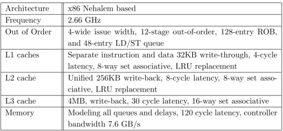
Table 1.Simulated CPU configuration
Architecture x86 Nehalem based Frequency 2.66 GHz
Out of Order 4-wide issue width, 12-stage out-of-order, 128-entry ROB, and 48-entry LD/ST queue
L1 caches Separate instruction and data 32KB write-through, 4-cycle latency, 8-way set associative, LRU replacement
L2 cache Unified 256KB write-back, 8-cycle latency, 8-way set asso-ciative, LRU replacement
L3 cache 4MB, write-back, 30 cycle latency, 16-way set associative Memory Modeling all queues and delays, 120 cycle latency, controller
bandwidth 7.6 GB/s
2.2. Data Generation
System simulators provide increased design flexibility compared to physical devices while offering detailed insights into runtime behaviors. An added benefit of using Sniper is the ability to output the statistics of different runtime behaviors (hereinafter referred to as attributes). Some of the statistics of interest include the number of micro operations (uops), branch prediction results, and cache and TLB accesses and misses. We have configured Sniper to periodically output a set of statistics that is generalized into nine ratio based attributes plus one IPC target value shown in Tab. 2. Generalizing the input attributes to the predictors enables predicting a workload’s performance on a certain core type while possibly using input from executions on a different core type but with the same ISA. For example, to predict how a thread currently executing on a large core will perform on a small core, the attribute values collected during the previous execution quantum on the large core are generalized into ratios and provided as input to the predictor for small core which outputs an estimated IPC on the small core. Ratio based attributes are also useful for conducting a system analysis based on the predictions for synthetic workloads that have different ratio values for the attributes.
2.3. Data Division
Before conducting any further data analysis, it is important to separate the data into a train set which we can poke into and analyze and a separate test set that will be used to evaluate the final models. Exploring the complete data without separating it into a train and test set biases any analysis due to a priori knowledge about the test set. A common technique is to set aside between 70%-80% of the data for the train set and 20%-30% for the test set. However, as described above, the two benchmark suites not only contain a different amount of individual benchmarks (26 SPEC2006 vs 13 SPLASH-2), but the completion times vary between the benchmarks as well. This results in different quantities of data samples available for each benchmark. As an additional measure to guard against biasing the training for the test set, instead of combining all the samples from all workloads into on large data set and then separating it into train and test sets, we separate the workloads themselves into different data sets. Therefore, the train set consists of roughly 70% or 19 benchmarks from SPEC2006 and 70% or 10 benchmarks from SPLASH-2. That leaves 7 SPEC2006 and 3 SPLASH-2 workloads for the test set. There are numerous possible combinations of which benchmarks to select for the train and test sets. To account for this, we train and evaluate the machine learning model 1000 different times each using a different combinations of benchmarks for the train and test sets chosen at random. The evaluation results in Section 3.3 are based on the averages and standard deviation of the 1,000 different train and test error results.
Another method for accounting for benchmark idiosyncrasies could be using an equal number of samples from each of the workloads in the train set during the learning phase. However, this would affect how representative the train set will be of the amount of time the system is executing the target workloads. It is important to note that any transformation on the train set such as normalization is also performed on the test set.
2.4. Data Exploration
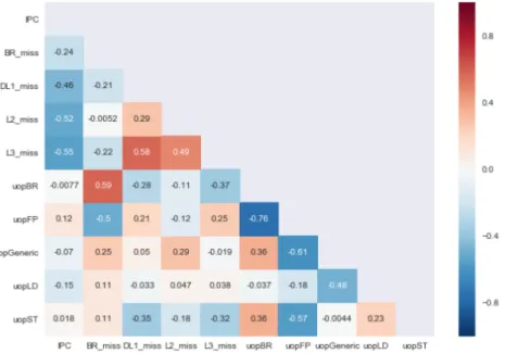
Exploring the data requires a mix of domain knowledge and utilizing several techniques with which to understand the distribution attributes and their relation to one another. Based on computer architecture domain knowledge, we can deduce that certain of the attributes may be highly correlated (e.g., IPC and L3 miss rate). Cleaning the data sets ensures that the amount of memory and computational overheads needed to work with the data sets is condensed. Removing noisy and/or redundant attributes can also be useful for reducing errors in our predictors later on.
Training and evaluating a simple linear regression model using IPC and each of the attributes independently can provide baseline error measurements and indicate whether it may be useful to apply non linear machine learning algorithms.
Figure 1.Pearson correlation heatmap of the attributes. The values of the attributes are based on ratio percentages (e.g., uopFP is the percentage of micro operations that are floating point)
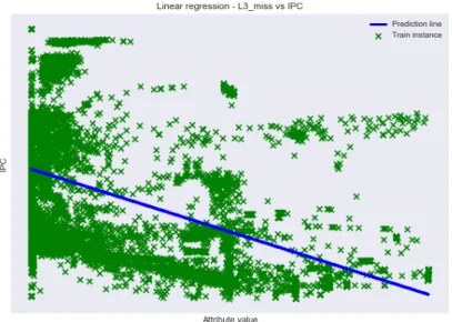
Figure 2 shows the linear regression predictors based on the L3 miss rate attribute which has the closest correlation with the IPC. The plot visualizes how the prediction line is not able to capture the non-linear relationship of the training data and target value for even the most correlated attribute. This observation is highlighted in Tab. 2 which presents the root mean square error (RMSE) on the training set for each of the separate linear models trained using an individual attribute as the input x and the IPC as the target y. The resulting errors are considerable given that they are around 0.7 and that the average IPC range is between 0 and 4. This reveals that there is an opportunity for improvement using machine learning predictors.
Figure 2. Scatter plot of L3 miss rate vs IPC from the training data set. Also plotted is the single-attribute (L3 miss rate) based linear regression prediction line in blue
Table 2.Runtime attributes expressed as ratio values collected each 1ms execution quantum. Also shows each attribute’s correlation with target IPC and the RMSE of the predictions against the training data set using simple linear regression
Attribute Correlation with IPC
Linear reg RMSE % uopLD -0.1538 0.7414
% uopST 0.0176 0.7502
% uopBR -0.0077 0.7503
% uopFP 0.1157 0.7453
% uopGeneric -0.0700 0.7485 BR miss % -0.2399 0.7284 DL1 miss % -0.4599 0.6663 L2 miss % -0.5172 0.6422 L3 miss % -0.5527 0.6253
3. A Case Study in Applying Machine Learning to Solve
Computer Architecture Problems
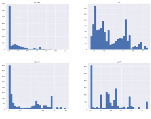
Figure 3. Histograms of the attributes branch misprediction rate, IPC, L3 miss rate, and per-centage of FP uops. They axis values are based on the quantity of instances from a total of over 13,000 samples which fall into the attribute range in the x axis
performance (measured in IPC) of a workload on an x86 core during an execution quantum. The goal of the predictor is to achieve low error and be able to predict using input data collected from executions on different core types. This enables cross core workload performance prediction which can be useful for a scheduler to improve system throughput. We analyze a set of popular machine learning algorithms, fine tune their learning and architectures, and lastly evaluate the final predictor errors.
3.1. Machine Learning Algorithms
In contrast to unsupervised learning which is useful for finding patterns in unstructured data, supervised training allows a machine learning model to learn to predict classes or values based on minimizing a loss function that quantifies the error between the predicted values and the target values. Since the data we have collected is labelled (i.e., the target IPC values are available in the data sets), we will focus on supervised machine learning methods. Moreover, since IPC is a continuous and not a categorical value, the machine learning models of interest are regressors, meaning they predict a continuous numerical value and not a class. Other areas in computer architecture may require the prediction of classes such as the case of branch prediction (i.e., a binary classification prediction of either branch taken or not taken).
machine learning algorithms is regulated throughhyperparameters which define the architecture of the specific algorithms. An overview of each of these algorithms and their hyperparameters is described below. All models are implemented using the Scikit-Learn Python framework [21] which offers a powerful toolbox of machine learning algorithms as well as preprocessing (e.g., normalization methods) and fine tuning methods (e.g., cross-validation and grid search meth-ods). Implementations for production purposes requiring strict timing constraints could instead implement the algorithms directly in a lower level language (e.g., C) and rely on hardware acceleration to reduce training and prediction latency.
3.1.1. Linear Regression Using Stochastic Gradient dDescent (SGD)
Stochastic gradient descent (SGD) is useful machine learning alternative for finding a linear model without having to utilize the normal equation which does not scale well with large data sets since it requires inverting an input matrix which carries a complexity of O(n2.3) to O(n3). This algorithm finds a linear function (e.g.,f(x) =w0+w1x1+w2x2+...+wnxn) that uses SGD
for training to learn the set of weightsw1...n that should be multiplied to every input parameter
x1...n and bias termw0. It is straightforward to implement and generally provides low variance but high error (i.e., bias), especially when used to approximate non linear functions. This model will use SGD to approximate a linear equation using all nine of the attributes plus an intercept term.
During training, the model predicts an output for every sample from the train dataset and compares it to the target value using a loss function. The result of the loss function is what the algorithm will try to minimize at every step of the training. Though we calculate the loss for every sample, the weights can be updated after every sample chosen randomly from the training data set (SGD), after calculating the sum of the losses for a subset of the total train data set (mini batch), or after calculating the sum of the losses for the entire train data set (full batch). Here we utilize SGD to update the weights.
For regression, we use the mean squared error loss functionM SE= m1 Pmi=1(yi−yˆi)2, where
m is the number of samples in the training batch,yi is the target IPC value, and the predicted
IPC value is ˆyi =w0+w1x1+w2x2+...+wnxn. To update the weights, the partial derivative of the
loss function with respect to the weight is multiplied with a learning rate hyperparameterαand then added to the old weight value. This is represented by the formulaw(inew) =wi+α∗∂M SE∂wi .
The learning rate may be either static (e.g., α = 0.01) or dynamically adjustable as is the case with momentum optimization [22]. The learning terminates when the algorithm converges to a minimum loss. This is always the case when using the MSE loss function for linear regression since it is a convex function. To prevent overfitting, especially for high dimensional training data sets, it is useful to add L1 (βPwj2) and/or L2 (βP|wj |) regularization terms to the loss
function to constrain the weights. Once trained, this linear model can be then used to make predictions by simply computing a weighed sum of the input parameters and a bias term. The principal hyperparameters of this model are the polynomial degree of the inputs, L1 and L2 regularization terms, loss function, and learning rate.
3.1.2. Decision Trees
the data to be normalized before training or predicting, thus reducing the amount of preparation time. The algorithm builds a binary tree node by node by focusing on a single attribute kand a threshold value for that attribute tk at a time. The algorithm relies on splitting the training
data set by using a loss function J which minimizes the MSE, J(k, tk) = mmlef tM SElef t + mright
m M SEright. A node’s MSE value is calculated by using the predicted value, ˆy is based on
averaging the target y value for allm instances belonging to that node.
Decision trees are simple to build and interpret. They also make it possible to rank the feature importances based on how close they are to the root of the tree (i.e., node depth). However, they are sensitive to rotations and small variations in the training data set which are aligned along non-orthogonal decision boundaries. Decision trees are non-parametric and also tend to overfit the training data set if left unconstrained during the construction of the binary tree. Reducing the degrees of freedom helps to reduce overfitting at the cost of increased error. A few interesting hyperparameters to help regularize the decision tree is setting its maximum depth and number of leaf nodes as well as the minimum number of instances a leaf or node must contain to split.
3.1.3. Random Forests
Random forests are an ensemble of shallow decision trees (i.e., estimators), each of which is trained on different random subset of the training data set and attributes. The technique for random sampling of the training data using replacement is known as bagging [2]. For this work, the random subsets are chosen using the random patches [14] technique which applies the bagging method to both training data and attributes. The output prediction of the random forest is the average of the predictions from all of the estimators. The increased diversity of the subsets and estimators results in larger individual bias (i.e., error) of each estimator but less variance overall than a single decision tree. This approach generally yields a better model than using a single decision tree except when features are highly correlated. It also tends to overfit if not adequately constrained. Random forests enable ranking feature importances by computing the average tree depth of a feature in all estimators. Their hyperparameters include many of those of the decision tree as well as the number of small decision trees estimators to use.
3.1.4. Artificial Neural Networks (ANNs)
ANN is a popular learning algorithm that is used to learn a non-linear function f(x) = y
through the use of training on an input set x and a target y. The relationships learned by the ANNs are often hard to identify and program manually, yet they can be lightweight and flexible to implement. They are capable of approximating complex non-linear functions and computing predictions quickly, but deep ANNs are also prone to overfitting the training data set.
An ANN consists of a set of input attributes (also known as input parameters)x1, x2, ..., xd
of d dimensions. In the fully-feedforward ANN that is implemented, all of these inputs are connected to every unit in the first hidden layer of the ANN, the outputs of each layer then connect to all the units of the next layer and so on in unidirectional fashion. Each input xi is
assigned a numerical weightwi,jfor its connection to unitj. The sum of all incoming connections
to a unit multiplied by their corresponding weight is then performed (zj =Pdi=1xi∗wi,j) before
being passed into the unit’s non-linear activate function h(zj). The activate function used in
compute and does not have a maximum saturation such as sigmoid or the hyperbolic tangent function which helps in reducing vanishing gradients during backpropagation (discussed below). The output of the activate function from the units from the lth layer is fed to the input of
the units of the (l+ 1)th layer. The final prediction is based on the outputs from all the units
of the last hidden layer without passing through the activation function. The weights of the ANN are randomly initialized using Glorot initialization [5] from a uniform distribution between +/−qn 6
inputs+noutputs .
To train an ANN, the backpropagation algorithm is utilized which defines a method to propagate the gradient of the loss function with respect to the ANN weights backwards from the final layer to the first. To update the weights, these partial derivatives, which represent the slope of the loss function with resect to the weights, are multiplied by the learning rate hyperparameter α and then added to the old weight value. This is represented by the formula
wi,j =wi,j +α∗ ∂M SE∂wi,j . Similar to linear regression using SGD, we can utilize stochastic, mini
batch, or full batch gradient descent to update the weights L1 and L2 regularization to reduce overfitting. Learning terminates upon convergence (when the partial derivatives have zero slope), after a given number of training epochs (an epoch is a full training pass over all batch iterations), or when the loss function of a validation set (discussed below) starts to steadily increase. The main ANN hyperparameters are the number of units, number of layers, activation function, loss function, batch size, regularization terms, and learning rate.
3.1.5. k-Nearest Neighbors (kNN)
The kNN algorithm predicts the IPC value for a new instance by firstly comparing its distance to all available data points and identifying the k-nearest data point neighbors. It then outputs the average of the IPC value of the k nearest data points as its prediction for the new instance. The distance formula used can vary (in this work the Euclidean one is used), but the dimensions of the inputs correspond to the number of attributes of the data points. The neighbors can be weighed either uniformly or by their distance to the new instance. The hyperparameter k acts to regularize the algorithm with a higher value generally reducing noise. Typically the kNN algorithm is one of the most straightforward machine learning methods to understand and implement. It is also advantageous because the algorithm is non-parameterized (i.e., does not make assumptions on the input data probability distribution) and easily adapts to changes in new data. The main drawbacks include prediction computation cost as well as its sensitivity to localized anomalies and biases. kNN is a lazy learning technique meaning that the computation is done at prediction time as opposed to training. To predict for a new instance, the algorithm must compute the distances of the new instance with all existing data points to find the nearest k neighbors.
3.1.6. Overheads
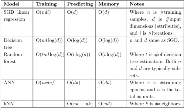
When deciding upon a model to implement to help solve a specific problem, it is critical to compare their overheads and see if they fall within the given problem’s constraints. This is especially the case in computer architecture where even minimal latency and memory overheads may outweigh the benefits of a proposed solution.
Table 3.Complexity overheads of machine learning models
Model Training Predicting Memory Notes
SGD linear regression
O(ndi) O(d) O(d) Where n is #training samples, d is #input dimensions (attributes), and i is #iterations. Decision
tree
O(ndlog(d)) O(log(d)) O(log(d)) n and d same as SGD.
Random forest
O(tndlog(d)) O(tlog(d)) O(tlog(d)) Where tis #of decision tree estimators. Both n
and dare typically sub-sets.
ANN O(nedu)) O(du) O(du) Where e is #training
epochs, and u is the to-tal # units.
kNN - O(nd +nk) O(nd) Wherek is #neighbors.
because the algorithms tend to perform several sequential iterations over the learning data set in order to reduce the loss function. As a greedy algorithm, however, kNN does not require to be trained to compute a prediction hence it has no training computational complexity. Conversely, kNN requires large prediction computational and memory complexity since it needs to calculate the distance between the new instance with all previous data points.
The computations for training and prediction are floating point arithmetic operations and the memory complexity represent the amount of data that needs to be stored and loaded. For example, an ANN composed of 11 input parameters, two hidden layers of 6 units and one output unit consists of about (11 + 1)∗ 6 + (6 + 1)∗6 + (6 + 1)∗1) = 121 floating point (FP) weights (the +1 is due to the bias term) needed to be stored and loaded. The amount of FP computations needed to be performed at each layer l of the ANN consists of a set of FP multiplication and addition operations, F P opsl = dlul+ (dl−1)ul, can be separated into
multiplication and addition FP ops. In this case,dl is the input dimension to the lth layer, and
ul is the number of units in the lth layer of the ANN. The computations needed for each ANN
prediction is (12∗6 + 11∗6) + (7∗6 + 6∗6) + (7∗1 + 6∗1) = 199 FP ops. It is up to the architect to analyze whether these computations and memory footprints can be handled in an efficient manner so as to keep the overheads within the constraints.
3.2. Model Validation and Fine Tuning
However, adjusting the hyperparameters based on how the algorithm predicts for the test data set will bias the training for the test data set. To make sure the testing data set is used for a final unbiased evaluation of the algorithms, the evaluation for fine tuning the models is made using a separatevalidation data set.
The validation data set is a random subset of the training data set that is kept aside (i.e., not used during the training phase) to evaluate the bias and variance of the algorithms. A more sophisticated and balanced validation method that is capable of using all of the training data for both training and evaluation is known as k-fold cross-validation. This method randomly splits the training data set intok subsets calledfolds. A model is then trainedk times using a different evaluation fold each time and training using the remainingk−1 folds. For example, to train an ANN using 5-fold cross validation, the training data set will be divided into 5 folds (i.e., 5 data subsets each containing 20% of the total instances in the training data set). The ANN model will be trained 5 different times, each time using a different fold for evaluation and the other four folds for training. The final k evaluation errors can be averaged to produce a single value and additionally provide a standard deviation precision measurement.
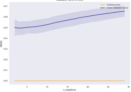
To fine tune a model, k-fold cross-validation can be combined with a hyperparameter grid search technique. The validation curves illustrate how different hyperparameter values affect a model’s training and validation errors. Deciding on a hyperparameter value using the validation curves is intuitive since the validation error curve will tend to decrease as the model becomes more powerful, but then increase at the point where the model complexity increases to the point of it overfitting. For example, based on the validation curve of the ANN in Fig. 4, the model chosen has 1 hidden layer of 100 hidden units. As is shown in the validation curve in Fig. 5, the kNN prediction error increases significantly after around k= 5. The hyperparameters of the other models were chosen using a similar grid search and validation curve analyses.
Figure 4. Validation curve of the ANN. The x axis ticks represent different models having (#hidden units, #hidden layers)
more of the training data. The learning curve for the SGD linear regression model is shown in Fig. 6. The shaded regions around the darker lines represent the standard deviations of the errors from the different cross-validation folds. Apparent from the figure is that as more train data is used during the training phase, the error decreases for the validation data set, but increases for the training data set. The standard deviations are also considerable due to the large variations between the instances and poor ability of the model to capture non linearities.
Figure 5.Validation curve of the kNN model. The x axis ticks represent values for k
Figure 6.Learning curve of the SGD linear regression model. As the model is able to train using more data, the error decreases for the validation data set but increases for the training data set
error (i.e., how high on theyaxis) the training error settles at, and the variance depends upon the gap between the training and validation curves. Greater bias indicate more error and greater variance denotes that the model has probably overfit to the training data and will perform significantly worse on unseen data than on the train set. A solution to high bias is to increase the complexity of the model and the number and/or quality of attributes and data. To reduce variance, it is often useful to simplify the model by reducing complexity or adding regularization, remove input attributes, and increase the diversity and quantity of the data. If the right tails of the learning curves do not settle, then adding more training data could serve to reduce the bias.
Figure 7.The feature importances of the random forest model
As mentioned previously, the decision tree and random forest algorithms are capable of ranking the importance of the input attributes. The feature importance of the trained random forest model is shown in Fig. 7. These relate closely to the correlations with the IPC that were shown in Tab. 2. If further reduction of attributes is desired (e.g., to reduce overfitting or computational or memory complexity), then feature importances will help to highlight the attributes which are most useful. For example, we could reduce the amount of attributes from 9 to 5 by keeping only those with importance value over 0.1. Then we could train a separate random forest model using these 5 attributes and compare the error and overhead results to decide which to implement.
Once a preferred set of input attributes and hyperparameters is identified using the com-bination of these techniques, a final version of the model is trained using the full training data set.
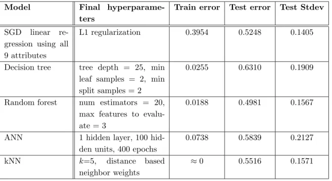
3.3. Final Model Results
and test data sets. In general, the models exhibit high variance but low bias especially compared to the single attribute linear regression predictors from Section 2.4.
Table 4.Final machine learning model results. Final hyperparameters and root mean squared error (RMSE) for models with original attributes and ratio transformed attributes
Model Final hyperparame-ters
Train error Test error Test Stdev
SGD linear re-gression using all 9 attributes
L1 regularization 0.3954 0.5248 0.1405
Decision tree tree depth = 25, min leaf samples = 2, min split samples = 2
0.0255 0.6310 0.1909
Random forest num estimators = 20, max features to evalu-ate = 3
0.0188 0.4981 0.1567
ANN 1 hidden layer, 100 hid-den units, 400 epochs
0.0738 0.5839 0.2127
kNN k=5, distance based
neighbor weights
≈0 0.5516 0.1571
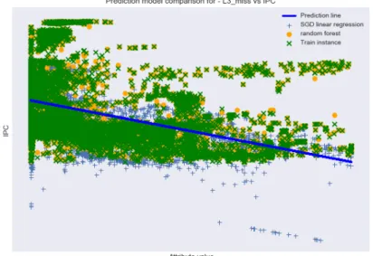
The significantly larger errors and standard deviation on the test set are curious and also indicative of high variance and could be the result of overfitting to the training set, but also that the diversity found in the training set unlike that contained in the test data set. Fig. 8 provides a 2-D visualization comparing how the SGD linear regressor and random forest models make their predictions as opposed to the simple single-feature linear regression model from Section 2.4. Apparent from the figure is that the machine learning based models, especially the random forest, tend to predict the training data exceptionally well but may also be a product of overfitting.
The k-nearest neighbors algorithm particularly suffers from high variance with nearly zero error on the training set and over 0.5 for the test. This is likely due to having many similar instances in the training data set. The training instances close to the testing instances also seemed to perform very differently which skewed the model’s prediction. The decision tree model also exhibits significant variance between the train and test errors. This is the case even after fine tuning the model using cross validation and a hyperparameter grid search, again due to poor representation of the test data within the training data set.
Figure 8. Scatter plot of L3 miss rate vs IPC from the training data set. Also plotted are the predictions based on the single-attribute linear regression, the multi-attribute SGD linear regression, and the random forest
The model that has the lowest prediction error on the test set is the random forest. SGD linear regression comes in at second, has the least variance between the train and test sets. However, it also suffers from an order of magnitude higher training error than any other models. In case of similar applications being frequently run on a system, the machine learning models would be able to predict significantly better than the SGD regressor, especially if making use of online learning. Though the random forest produces the least amount of test prediction error, any final implementation choice will depend upon a careful comparison of the target benchmarks, errors, and performance and space requirements.
3.4. Exploiting the Predictors
Once a final predictor has been chosen to be implemented, a mechanism must be identified which is able to exploit the extra system knowledge and translate it into system efficiency gains. The added knowledge gained thanks to the use of a predictor such as an ANN, is the IPC value for a benchmark on a hardware core for an execution quantum. A useful mechanism to exploit knowing how well workloads would perform on different core types would be a resource manager such as a CPU scheduler for heterogeneous systems. Given that several workloads may be running concurrently on a heterogeneous system composed of several cores of different types, the scheduler can utilize a specific IPC predictor per core type to predict how the workloads will perform on all other core types. The scheduler can then compare all the different possible workload to core mapping combinations and choose the one that results in the highest system IPC.
exploited by mechanisms to improve system performance are in the area of branch prediction [9] and cache line reusability [10, 25]. Knowledge is powerful when exploited adeptly.
4. Related Work
The application of machine learning to the field of computer architecture is currently in its inceptive stages with the few exploratory studies showing impressive promise. Recently, there has been pioneering studies conducted on applying machine/deep learning to CPU scheduling. In the works [18, 19] artificial neural network performance predictors are used by the scheduler to improve the system throughput over a Linux based scheduler by over 30%. Other approaches to using machine/deep learning for scheduling has been to classify applications, as well as to identify process attributes and a program’s execution history. This is the approach of [17] which used decision trees to characterize whole programs and customize CPU time slices to reduce application turn around time by decreasing the amount of context swaps. The work presented in [12] studies using structural similarity accuracy values and support vector machines and linear regression to predict thread performance on different core types at a high granularity level (1 second). In the study [6], CPU burst times of whole jobs for computational grids are estimated using a machine learning approach. An approach that utilized machine learning for selecting whether to execute a task on a CPU or GPU based on the size of the input data is done by Shulga et al. [24]. Fedorova et al. [4] proposes an algorithm that uses reinforcement learning to maximize normalized aggregate IPC. They demonstrate the need for balanced core assignment but do not provide an implementation.
For branch prediction, Jimenez et al. [9] proposed using a perceptron based predictor in order to improve CPU performance. Several studies have applied machine learning for the purpose of cache management. In the work [10, 25] the authors propose perceptron learning for reuse prediction and also present a prediction method for future reuse of cache blocks using different types of parameters. Predicting L2 cache behavior is done using machine learning for the purpose of adapting a process scheduler for reducing shared L2 contention in [23].
Conclusion
The revitalization of machine learning has led to a vast and diverse set of useful applications that affect daily lives. The ability of the algorithms to learn complex non-linear relationships between the attributes of the data and the target values has led to them being utilized as powerful prediction models. While there has been much interest recently in accelerating machine learning algorithms with custom hardware, there have been few applications of machine learning to improve system performance.
The goal of this paper has been to serve as a foundational base and guide to future computer architecture research seeking to make use of machine learning models for improving system efficiency. We have described a process to highlight when, why, and how to utilize machine learning models for improving system performance and provided a relevant example showcasing the ability of machine learning based cross core IPC predictors to help enable CPU schedulers to improve system throughput.
We have analyzed a set of popular machine learning models including stochastic gradient descent based linear regression, decision trees, random forests, artificial neural networks, and
com-putational and memory complexities, and a process to fine tune and evaluate the models. After comparing the results of the predictors, the random forest narrowly produces the lowest root mean squared error in its testing predictions. Finally, we discussed how the predictor can be exploited by a mechanism such as a scheduler for heterogeneous systems in order to improve the overall system performance.
For future work, reinforcement learning may be a fruitful option to explore in using machine learning to improve scheduling. Predicting application performance and energy consumption, cache accesses, memory and I/O latencies, branch conditions, and interference effects between threads are just a few examples of useful knowledge that can help to improve system performance and energy efficiency if adequately exploited. In addition, testing the implementations on real systems is a pragmatic approach forward that helps to validate and continue pioneer applying machine learning to computer architecture.
Acknowledgements
This work has been supported by the European Research Council (ERC) Advanced Grant RoMoL (Grant Agreemnt 321253) and by the Spanish Ministry of Science and Innovation (con-tract TIN 2015-65316P).
This paper is distributed under the terms of the Creative Commons Attribution-Non Com-mercial 3.0 License which permits non-comCom-mercial use, reproduction and distribution of the work without further permission provided the original work is properly cited.
References
1. Abadi, M., Barham, P., Chen, J., Chen, Z., Davis, A., Dean, J., Devin, M., Ghemawat, S., Irving, G., Isard, M., Kudlur, M., Levenberg, J., Monga, R., Moore, S., Murray, D.G., Steiner, B., Tucker, P.A., Vasudevan, V., Warden, P., Wicke, M., Yu, Y., Zhang, X.: Tensorflow: A system for large-scale machine learning. CoRR abs/1605.08695 (2016), http://arxiv.org/abs/1605.08695, accessed: 2018-03-01
2. Breiman, L.: Bagging predictors. Machine Learning 24(2), 123–140 (Aug 1996), DOI: 10.1007/bf00058655
3. Carlson, T.E., Heirman, W., Eeckhout, L.: Sniper: exploring the level of abstraction for scalable and accurate parallel multi-core simulation. In: Proceedings of 2011 International Conference for High Performance Computing, Networking, Storage and Analysis on - SC. ACM Press (2011), DOI: 10.1145/2063384.2063454
4. Fedorova, A., Vengerov, D., Doucette, D.: Operating system scheduling on heterogeneous core systems. In: Proceedings of the Workshop on Operating System Support for Heteroge-neous Multicore Architectures (2007), http://citeseerx.ist.psu.edu/viewdoc/summary?doi= 10.1.1.369.7891
Sardinia, Italy. Proceedings of Machine Learning Research, vol. 9, pp. 249–256. PMLR (2010), http://proceedings.mlr.press/v9/glorot10a.html, accessed: 2018-03-01
6. Helmy, T., Al-Azani, S., Bin-Obaidellah, O.: A machine learning-based approach to estimate the CPU-burst time for processes in the computational grids. In: 2015 3rd International Conference on Artificial Intelligence, Modelling and Simulation (AIMS). IEEE (Dec 2015), DOI: 10.1109/aims.2015.11
7. Henning, J.L.: SPEC CPU2006 benchmark descriptions. ACM SIGARCH Computer Archi-tecture News 34(4), 1–17 (Sep 2006), DOI: 10.1145/1186736.1186737
8. Jia, Y., Shelhamer, E., Donahue, J., Karayev, S., Long, J., Girshick, R., Guadarrama, S., Darrell, T.: Caffe: Convolutional architecture for fast feature embedding. In: Proceedings of the 22Nd ACM International Conference on Multimedia. pp. 675–678. MM ’14, ACM, New York, NY, USA (2014), DOI: 10.1145/2647868.2654889
9. Jimenez, D.A., Lin, C.: Dynamic branch prediction with perceptrons. In: Proceedings HPCA Seventh International Symposium on High-Performance Computer Architecture. pp. 197–206. IEEE Comput. Soc (2001), DOI: 10.1109/HPCA.2001.903263
10. Jim´enez, D.A., Teran, E.: Multiperspective reuse prediction. In: Proceedings of the 50th Annual IEEE/ACM International Symposium on Microarchitecture - MICRO-50. pp. 436– 448. ACM Press (2017), DOI: 10.1145/3123939.3123942
11. LeCun, Y., Bengio, Y., Hinton, G.: Deep learning. Nature 521(7553), 436–444 (May 2015), DOI: 10.1038/nature14539
12. Li, C.V., Petrucci, V., Mosse, D.: Predicting thread profiles across core types via machine learning on heterogeneous multiprocessors. In: 2016 VI Brazilian Symposium on Computing Systems Engineering (SBESC). IEEE (Nov 2016), DOI: 10.1109/sbesc.2016.017
13. Linden, G., Smith, B., York, J.: Amazon.com recommendations: item-to-item collaborative filtering. IEEE Internet Computing 7(1), 76–80 (Jan 2003), DOI: 10.1109/mic.2003.1167344
14. Louppe, G., Geurts, P.: Ensembles on random patches. In: Machine Learning and Knowledge Discovery in Databases, pp. 346–361. Springer Berlin Heidelberg (2012), DOI: 10.1007/978-3-642-33460-3 28
15. Misra, J., Saha, I.: Artificial neural networks in hardware: A survey of two decades of progress. Neurocomputing 74(1-3), 239–255 (Dec 2010), DOI: 10.1016/j.neucom.2010.03.021
16. Mnih, V., Kavukcuoglu, K., Silver, D., Graves, A., Antonoglou, I., Wierstra, D., Riedmiller, M.A.: Playing atari with deep reinforcement learning. CoRR abs/1312.5602 (2013), http: //arxiv.org/abs/1312.5602, accessed: 2018-03-01
17. Negi, A., Kumar, P.: Applying machine learning techniques to improve linux process scheduling. In: TENCON 2005 - 2005 IEEE Region 10 Conference. pp. 1–6. IEEE (Nov 2005), DOI: 10.1109/tencon.2005.300837
In: 2017 29th International Symposium on Computer Architecture and High Performance Computing (SBAC-PAD). pp. 121–128. IEEE (Oct 2017), DOI: 10.1109/sbac-pad.2017.23
19. Nemirovsky, D., Arkose, T., Markovic, N., Nemirovsky, M., Unsal, O., Cristal, A., Valero, M.: A deep learning mapper (DLM) for scheduling on heterogeneous systems. In: Commu-nications in Computer and Information Science, pp. 3–20. Springer International Publishing (Dec 2017), DOI: 10.1007/978-3-319-73353-1 1
20. Ovtcharov, K., Ruwase, O., Kim, J.Y., Fowers, J., Strauss, K., Chung, E.S.: Toward accel-erating deep learning at scale using specialized hardware in the datacenter. In: 2015 IEEE Hot Chips 27 Symposium (HCS). IEEE (Aug 2015), DOI: 10.1109/hotchips.2015.7477459
21. Pedregosa, F., Varoquaux, G., Gramfort, A., Michel, V., Thirion, B., Grisel, O., Blondel, M., Prettenhofer, P., Weiss, R., Dubourg, V., Vanderplas, J., Passos, A., Cournapeau, D., Brucher, M., Perrot, M., Duchesnay, E.: Scikit-learn: Machine learning in python. The Journal of Machine Learning Research 12, 2825–2830 (Nov 2011), http://dl.acm.org/ citation.cfm?id=1953048.2078195, accessed: 2018-03-01
22. Polyak, B.: Some methods of speeding up the convergence of iteration methods. USSR Computational Mathematics and Mathematical Physics 4(5), 1–17 (Jan 1964), DOI: 10.1016/0041-5553(64)90137-5
23. Rai, J.K., Negi, A., Wankar, R., Nayak, K.D.: A machine learning based meta-scheduler for multi-core processors. International Journal of Adaptive, Resilient and Autonomic Systems 1(4), 46–59 (Oct 2010), DOI: 10.4018/jaras.2010100104
24. Shulga, D.A., Kapustin, A.A., Kozlov, A.A., Kozyrev, A.A., Rovnyagin, M.M.: The schedul-ing based on machine learnschedul-ing for heterogeneous CPU/GPU systems. In: 2016 IEEE NW Russia Young Researchers in Electrical and Electronic Engineering Conference (EICon-RusNW). IEEE (Feb 2016), DOI: 10.1109/eiconrusnw.2016.7448189
25. Teran, E., Wang, Z., Jimenez, D.A.: Perceptron learning for reuse prediction. In: 2016 49th Annual IEEE/ACM International Symposium on Microarchitecture (MICRO). IEEE (Oct 2016), DOI: 10.1109/micro.2016.7783705
26. Woo, S., Ohara, M., Torrie, E., Singh, J., Gupta, A.: The SPLASH-2 pro-grams: characterization and methodological considerations. In: Proceedings 22nd An-nual International Symposium on Computer Architecture. pp. 24–36. ACM (Jun 1995), DOI: 10.1109/isca.1995.524546