94
Production Optimization for Plan of Gas Field Development Using Marginal
Cost Analysis
Suprapto Soemardan
1, Widodo Wahyu Purwanto
1*, and Arsegianto
21. Chemical Engineering Department, Faculty of Engineering, Universitas Indonesia, Depok 16424, Indonesia 2. Petroleum Engineering Study Program, Institut Teknologi Bandung, Bandung 40116, Indonesia
*E-mail: [email protected]
Abstract
Gas production rate is one of the most important variables affecting the feasibility plan of gas field development. It take into account reservoir characteristics, gas reserves, number of wells, production facilities, government take and market conditions. In this research, a mathematical model of gas production optimization has been developed using marginal cost analysis in determining the optimum gas production rate for economic profit, by employing the case study of Matindok Field. The results show that the optimum gas production rate is mainly affected by gas price duration and time of gas delivery. When the price of gas increases, the optimum gas production rate will increase, and then it will become closer to the maximum production rate of the reservoir. Increasing the duration time of gas delivery will reduce the optimum gas production rate and increase maximum profit non-linearly.
Abstrak
Optimisasi Produksi untuk Perencanaan Pengembangan Lapangan Gas dengan Analisis Biaya Marginal. Laju
produksi merupakan salah satu variabel penting yang mempengaruhi kelayakan perencanaan pengembangan lapangan gas berdasarkan atas karakteristik reservoir, jumlah sumur, fasilitas produksi, kondisi pasar dan memenuhi porsi penerimaan pemerintah. Dalam penelitian ini suatu model matematika optimisasi produksi gas dikembangkan untuk menentukan laju produksi gas optimum berdasarkan pendekatan analisis biaya marginal yang mengacu pada keuntungan ekonomi, khususnya untuk kasus kajian di lapangan gas Matindok.. Hasil penelitian memperlihatkan bahwa laju produksi gas optimum sangat tergantung harga gas dan durasi lamanya pengiriman gas. Ketika harga gas naik, laju produksi gas optimum akan naik dan mendekati laju produksi maksimum reservoir. Peningkatan durasi pengiriman gas akan menurunkan laju produksi gas optimum dan meningkatkan keuntungan maksimumnya secara non-linear.
Keywords: marginal cost, natural gas fields, production optimization
1.
Introduction
Accurate planning of gas field development is not only dependent on the characteristics of the reservoir, but also on proper emphasis of cost allocation for each work activities of gas production capacity [1-2].
Several studies have been conducted to optimize the gas business through a variety of methods. These include surveys of the literature dealing with the optimization of petroleum and natural gas production; drilling, reservoir simulation, production planning and operations, enhanced recovery processes [3]; the daily production rates for an offshore oilfield to achieve a production
optimal production rate is greatly influenced by the contract terms, and at the optimal rate the production is in a plateau phase. Abdel Sabour [9] showed that marginal cost analysis can be used to create a model to estimate the optimum mine size. The model was developed on the basis of marginal analysis, assuming that the optimum level of production is a condition in which the present value of the marginal cost is equal to the present value of marginal revenue.
The aim of this paper is to develop a model of gas production optimization to solve the optimum gas production rate using marginal cost analysis.
Marginal Cost Model: Cost curves. Fig. 1 shows the
total cost curve versus gas production rate of the developed gas field. In the early stage of field development, some expenses have been paid, while the exploration stage for discovery of the gas reserve is considered as a fixed cost. Primary production will entail costs to set up the production facility. This stage is called the high cost for low production zone.
The fully developed stage of high daily production, which is approaching the reservoir’s maximum capacity, will impose a substantial cost for numerous production wells, environmental handling, treatment of CO2 and H2S, and the possible addition of compressed
gas in the declining reservoir pressure phase. This stage is called the high cost for high production zone. Between the intervals of the high cost for low
production zone and the high cost for high production zone, there is the effective stage where the additional
cost of adding gas production will be lower than the previous stages. The zone between the two stages is called the cost effective zone.
Total Cost (TC) is generated by the sum of Fixed Cost (FC) and Variable Cost (VC) [10]. Fixed costs are the costs of identifying gas reserves through seismic and exploration activity, whereas variable costs are the costs of field development and operations/maintenance.
VC
FC
TC
=
+
(1)Total cost for each production unit (TC/Qgcum) will be very high at the low production zone and will decrease in the effective production zone; however it will rise again at the high production zone. Average cost (AC) is the cost for each production unit of gas, while marginal cost (MC) refers to the total additional cost as a result of the increase in one unit of gas produced [11-12].
cum
Qg TC
AC= (2)
dQg dTC
MC = (3)
Fig. 1. The Fixed Cost, Variable Cost and Total Cost Versus Gas Production Rate
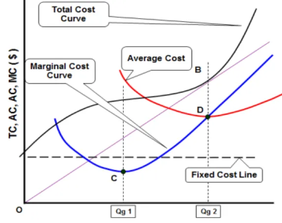
Fig. 2. Curves of Total Cost, Marginal Cost and Average Cost
Each curve of total cost (TC), average cost (AC), and marginal cost (MC) are illustrated in Fig. 2. Value and curve shape of TC is very dependent on gas rate and time of delivery; therefore, AC and MC also depend on
Qg and TP. TC is non-linear to Qgcum, and AC and MC are non-linear to Qg or Qgcum. In particular, the MC curve will cross the AC curve at the minimum point of
AC in the D point. The D point will give the Qg2 as the recommended minimum gas rate (Qgmin-rec) which is based on the reservoir capacity and costs incurred. At the point of D, there shall be applied dAC/dQg = 0.
Total and marginal revenue. Total revenue is revenue
earned from all products (gas and condensate) in monetary units. It is written as:
TR = (GP × Qgcum) + (CP × Qccum) (4)
total cumulative gas production (mscf) and cumulative condensate production (bbl).
Condensate production rate (Qc) in Eq. (4) is predicted using condensate/gas ratio (CGR) multiplied by gas production rate (Qg), and is written:
Qc = Qg × CGR (5)
Where: Qc in bbl/d and the CGR in bbl/mmscf depend on reservoir type. For dry-gas and wet-gas reservoirs, condensate rate is generally linear to gas deliverability, with CGR considered constant during gas production [13-15]. For the gas-condensate reservoir type, condensate rate can be predicted by Boogar’s equation [16], where
CGR will remain constant at pressure above the dew
point. When pressure drops below the dew point, the
CGR will decline depending on the reservoir pressure.
Marginal Revenue (MR) is the result of differentiating incremental total revenue to additional gas production rate as given in the equation:
dQg dTR
MR = (6)
Gas price and condensate price. Gas price should
preferably be set higher than the minimum gas price (GPmin). The GPmin is most likely acceptable to all stakeholders, both government and the oil and gas producer. GPmin is calculated from production cost (PC), risk factor during exploration (ER), the return on costs (ROC), and what the government takes (GT), so that the
GPmin can be written as follows:
GT ER ROC PC
GPmin= + + + (7)
Where GPmin, PC, ROC, ER and GT are in $/mscf or $/mmbtu. The ROC is determined from %ROC × PC and the ER is calculated from %ER × PC. The %ROC and %ER is determined by the operator on its investment policy. GT is estimated from (%BN / %BO) × ROC, where %BN is the portion the government takes and %BO is the operator’s portion. The government’s portion is based on the oil and gas mining contract subject to the Law of Oil and Gas.
Gas price may be formulated as follows:
× + + + × ≥ ROC BO BN ER ROC PC GP % % % % %
1 (8)
PC is calculated by Eq. (9) as follows:
) (Qgcum
TC
PC= (9)
Boucher [17] emphasizes that the gas price needs to be carefully considered by the prospective users of gas in terms of willingness to pay to generate the best price, and considering the long-term economics.
Optimum production rate. Optimum gas production
rate (Qgopt) is defined as gas production rate which results in maximum profit (π) for the operator as investor without reducing the government’s portion. Profit for the operating party means that total cost is deducted from total revenue and multiplied by the operator’s portion (%BO):
) (
%BO × TR −TC
=
π
(10)Where: %BO + %BN = 1.
Furthermore, Eq. (10) is differentiated to incremental gas rate; then, considering Eqs. (3) and (6), then:
) (
%BO MR MC
dQg d − × = π (11)
Mathematically, maximum profit (πmax) will occur at the gas rate point where the increasing gas rate has no more influence on profit, either positive or negative. In other words, optimum gas production rate (Qgopt) will occur when dπ / dQg = 0, or MR = MC, which will also
generate maximum profit. The maximum profit is a function of TR which contains the gas price; thus, the value of πmax will highly depend on gas and condensate prices.
2. Methods
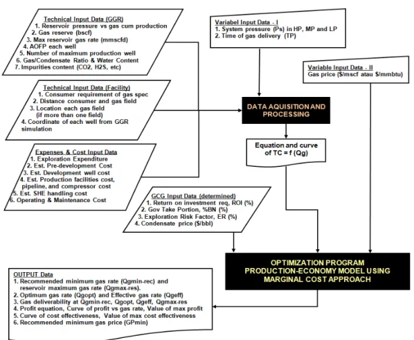
This study uses the case of development planning of Matindok Field in Central Sulawesi, which is one of the suppliers to LNG plants [18]. Fig. 3 is a schematic diagram for solving the optimization of gas production planning by the following steps:
Data acquisition and processing. There are three kinds
of data that are input in the data acquisition and analysis process. Technical data consist of geology-reservoir data which result from Geology-Geophysics-Reservoir (GGR) analysis and simulation. Other technical data include production facility data required by the production system [13-15]. Several engineering data in Matindok Field are summarized in Table 1 [18].
Fig. 3. Schematic Diagram of Gas Field Development Using Marginal Cost Approach
Table 1. Summary of Engineering Data in Matindok Field
Description Code, Formula Value Unit
Gas Reserve (90%P1+50%P2) Calculated 236.44 bscf
Maximum Gas Deliverability Calculated 196.25 bscf Bottom Hole Pressure
Estimated Well Max Capacity
well test well test
2,725 35.74
psi mmscfd Reservoir Expansion Factor (Bg) test lab 0.0082738 cuft/scf
CO2 Content test lab 5 Mol%
H2S Content test lab 4,000 ppm
Gas-condensate ratio Water Content
well test from the DST
71,400 (wet gas) See curve
Scf/bbl bbl/mmscf
High X > 800 psi
Medium 400<X<800 psi Pressure System
Low 400 psi
Well production capacity 20% of AOFP Max 10 mmscfd/well Note: AOFP = Absolute Open Flow Potential, DST = Drill Stem Test
Variable costs consist of well development, production facilities, pipeline, land acquisition and preparation, utilities, and allocated cost for plant abandonment. All are determined according to the amount of gas produced based on reservoir capacity. Production facility costs are
mainly flow line and pipeline, Acid Gas Removal Unit and Sulfur Recovery Unit (AGRU/SRU), water treatment unit, booster compressor, and CO2 injection
development well is around $5,600 per meter of depth [18]. The operating costs consist of direct operating for gas and condensate production, handling for produced water, CO2 compression to reservoir, H2S handling,
AGRU-SRU operation, and insurance of assets. Direct operating costs also cover all costs for production and processing, pipeline, utilities, operation and maintenance for all equipment, and booster compressor.
From the acquisition and processing steps, an equation and curve of TC and gas deliverability patterns will result in maximum reservoir gas rate. The equation and curve of TC will be the main object that will be solved.
Gas deliverability estimation. A gas deliverability
scenario is based on pressure system and duration time desired by agreement between the gas producer and consumer. Reservoir pressure and pressure drop for each gas flow rate is set for each gas reservoir. Reservoir engineering knowledge [16-17] has correlated
between Bottom Hole Flowing Pressure (BHFP) and cumulative gas production (Qgcum) by:
i
cum BHFP
Qg m Z
BHFP / =− ( )+( ) (12)
After correlation among reservoir pressure, Qgcum, remaining gas reserve at every flow rate (Qg), and the number of production wells which can be drilled, it is then necessary to install the production facilities, including booster compressor and pipeline. Qgcum is calculated from gas deliverability during production year based on the reservoir characteristics using petroleum engineering practice [14] and Boogar’s approach [16]. When reservoir pressure has dropped below the pressure system setting, the gas compressor should then be installed to increase outlet pressure up to the pressure setting. The remaining gas reserve is calculated by deducting the initial reserve from Qgcum at the pressure condition of the reservoir.
Table 2. Realization Exploration Costs and Estimated Development Well for Matindok Field
Well Depth (m) Cost
(million $) Remarks
Existing wells 5.5 Exploration well
MTD-2 2,200 12.5 Delineation vertical well
MTD-3 2,347 13.4 New directional well
MTD-4 2,235 12.7 New vertical well
MTD-5 2,235 12.7 New directional well
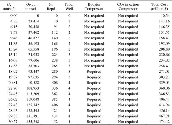
Table 3. Qg and TC Data Summary in Matindok Field for 15 Years
Qg mmscfd
Qgcum mmscf
Qc Bcpd
Prod. Well
Booster Compressor
CO2 injection Compressor
Total Cost (million $)
Correlation of gas production and total cost. Based on estimated gas production rate and total cost at time of gas delivery, the correlation of the polynomial equation is adopted by using MATLAB within an accuracy of R2. The polynomial equation is a third-order equation. Based on the equation of total cost and cumulative gas production rate, marginal cost (MC), average cost (AC), and minimum gas price (GPmin) should have a polynomial equation using Eqs. (2), (3), and (7).
Production rate optimization. The optimum production rate is obtained by maximizing the objective function of profit (π) as explained in the previous section. Gas price (GP) and duration time of gas delivery (TP) are put in exogenous variables. There are also GCG input data as constant variables, such as government take portion (%BN) as stipulated in the contract, return on cost (ROC), and exploration risk factor (%ER) determined by operator requirement.
The equation of TR as a function of Qg can be generated by a computer program using a one-dimensional, non-linear model. After that, the value ofπ can be estimated for each Qg by using Eq. (10). The recommended minimum gas rate (Qgmin-rec), the effective production rate (Qgeff), the optimum gas production rate (Qgopt) and the maximum profit (πmax) can be estimated from the equation of π. Maximum and minimum gas production rates of the reservoir and a combination of contract terms will be constraints in this research.
3. Results and Discussion
Cost curve. For a duration of 15 years, the estimated
Qg and TC is made in 20 data points about the total of
capital and operating costs for each gas rate as shown in Table 3. The equation of total cost as a function of cumulative gas production rate is represented in Fig. 4.
TC = 3.11E-7(Qgcum)3 - 0.056(Qgcum)2 +
5,449(Qgcum) + 10.54E6 (13)
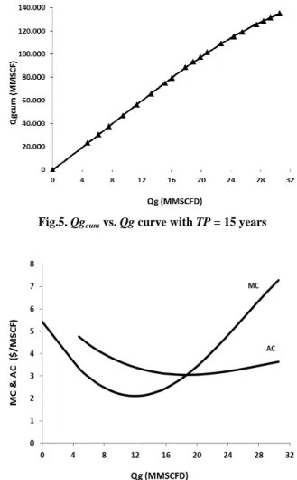
To simplify, the correlation between gas rate and cumulative produced gas can be shown in Fig. 5 and its correlation can be written as:
Qgcum = -1.76Qg3 + 44.02Qg2 + 4,702 Qg + 85.29 (14)
Average and marginal cost. The average cost (AC) and
marginal cost (MC) according to Eqs. (2) and (3) can be determined from the equation of total cost in Eq. (13). The equations of AC and MC are as follows:
AC = 3.11E-7(Qgcum)2 - 0.056(Qgcum) + 5,449 + 05E7(Qgcum)-1 (15)
MC = 9.34E-7(Qgcum)2 - 0.112(Qgcum) + 5,449 (16)
MC and AC curves in function Qg are obtained from
Eqs. (14), (15), and (16) as shown in Fig. 6. From the
AC curve, we get point ACmin at about $3.05/mscf at
Fig. 4. TC vs. Qgcum Curve in Matindok Field with TP = 15 Years
Fig.5. Qgcum vs. Qg curve with TP = 15 years
Fig. 6. MC and AC vs. Qg in Matindok Field with TP = 15 Years
Gas price and total revenue. Given that Production
Sharing Contractor (PSC) policy for the ROC is 16%,
ER is 10%, GT is 67.5%, then the GPmin at Matindok Field for various durations of gas delivery can be simulated using equations (7) and (8). Fig. 7 shows minimum gas price (GPmin) at each Qg for Matindok Field with TP = 15 years compared to average cost (AC). The GPmin of around $5.49/mscf occurs when recommended gas rate (Qgmin-rec) = 18.67 mmscfd. At another gas production rate, the gas price will be higher than $5.49/mscf.
By putting in values of gas price (GP), condensate price (CP), cumulative gas (Qgcum) and cumulative condensate (Qccum), total revenue will be identified from Eq. (4). Fig. 8 shows TR curve versus Qg and then the equation of TR can be obtained:
TR = -10,798Qg3 + 26,6136 Qg2 + 3E+07Qg (23)
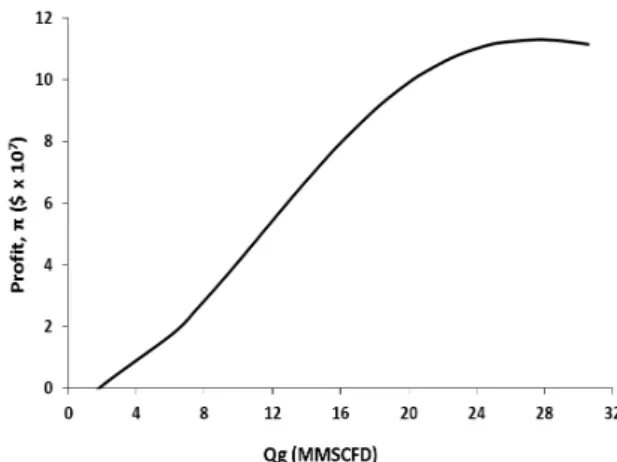
Optimum gas production. Based on TC and TR, profit
(π) can be determined by Eq. (10). For GP = $5/mscf,
CP = $80/bbl, TP = 15 years and the government’s take
portion (%BN) is 67.5%, the profit curve will be as shown in Fig. 9. The profit will increase if gas production
Fig. 7. Average Cost and Minimum Gas Price vs. Qg Plateau at Ps = 800psi, GP = $5/mscf, CP = $80/bbl,
TP = 15 Years
Fig. 8. TC, TR and π vs. Qg in Matindok Field at GP = $5/mscf, CP = $80/bbl, TP = 15 Years
Fig. 9. Profit vs. Qg in Matindok Field at GP = $5/mscf,
CP = $80/bbl and TP = 15 Years
Fig. 10. Gas Deliverability in Matindok Field at GP = $5/mscf, CP = $80/bbl, TP = 15 Years. Qgmax-res (––––), Qgopt ( ), and Qgmin-rec ( )
rate increases. However, it can be seen that the profit will reach a maximum value at a certain gas production rate. The maximum profit (πmax) is about $114.9 million and the prediction of optimum gas production rate (Qgopt) will be at 27.63 mmscfd.
Fig. 10 shows how the position of optimum gas rate (Qgopt) compares to another gas rate position such as minimum gas rate (Qgmin-rec), and maximum reservoir gas rate (Qgmax-res).
Factors influencing optimum production rate
.
If the gas price increases from $4 to $8/mscf and condensate price is kept at $80/bbl, the values of Qgopt and πmax are shown in Table 4. The gas can generate a maximum profit that becomes higher and higher at the high value of GP.Profit is highly dependent on the prices of gas and condensate. For example, if GP is raised to $5.5/mscf then π will increase to $135.9 million and optimum flow rate will be at 28.84 mmscfd. Increasing gas prices will
G
a
s
R
a
te
(
M
M
S
C
F
D
)
Project Time (year) 35 -
1 3 5 7 9 11 13 15 30 -
25 -
20 -
15 -
10 -
5 -
generate an optimum production rate (Qgopt) closer to the maximum production rate of the reservoir (Qg
max-res). The table also presents that a gas price around $6/mscf will generate Qgopt equal to Qgmax-res, 30.57 mmscfd, with πmax around $155.2 million. In contrast, a
GP = $5/mscf will generate Qgopt < Qgmax-res. This condition can be explained by observing that the gas price of $6/mscf has exceeded the previously-calculated minimum gas price of $5.49/mscf. Therefore, Qgopt =
Qgmax-res and total cost will stabilize at the same value when the gas price is higher than the minimum.
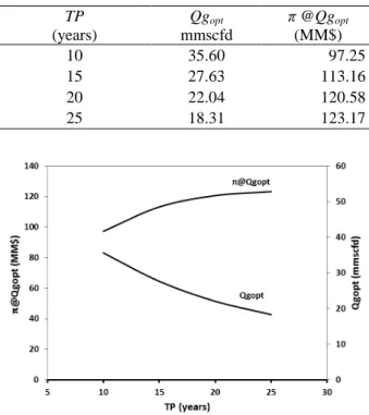
Duration time of gas delivery affects the optimum production rate as shown in Table 5. By increasing the duration of gas delivery, the optimum gas rate will be decreased non-linearly, while the maximum profit will rise sharply at TP less than 20 years. The values then tend toward constant at TP greater than 20 years, as shown in Fig. 11.
Table 4. Impact of Gas Price (GP) on Optimum Gas Production Rate at CP = $80/bbl, TP = 15 Years
GP
$/mscf
Qgopt mmscfd
Qgmax mmscfd
π@ Qgopt (MM$)
π@Qgmax (MM$)
4 25.09 30.56 73.65 67.25
5 27.63 30.56 113.16 111.26
6 30.57 30.56 155.25 155.25
7 30.57 30.56 199.23 199.23
8 30.57 30.56 243.20 243.20
Table 5. Impact of TP on Optimum Production Rate with
GP @ $5/mscf and CP @ $80/bbl
TP
(years)
Qgopt mmscfd
π @Qgopt (MM$)
10 35.60 97.25
15 27.63 113.16
20 22.04 120.58
25 18.31 123.17
Fig. 11. Effect of Time of Gas Delivery on Optimum Gas Rate and Maximum Profit in Matindok Field
4. Conclusions
In this paper, we estimated the empirical cost function based on technical and economic data of gas field development. The optimization based on marginal cost was done to find the optimum gas production rate for given constraints and exogenous variables.
The optimization results revealed that the optimum production rate was greatly influenced by the gas price and duration time of gas delivery.It was found that as the gas price increased by $1/mmscf, gas production rate increased by 10% and then tended closer to the maximum production rate of the reservoir. At the range of reservoir ability, increasing duration time of gas delivery will reduce the optimum gas production rate and increase maximum profit non-linearly.
The analysis of the relationship between exogenous variables and optimum production rate is helpful for companies in negotiating gas prices in contracts. It provides vital information for companies developing a gas field strategy.
Acknowledgments
The author (Soemardan) wishes to express many thanks to the Matindok Gas Development Project of PERTAMINA EP during his (Soemardan) position as Field Development Manager from 2003-2008, Prof. Widjajono Partowidagdo (Petroleum Department ITB) for his support and guidance during this research, and Mr. Abdullah (Mathematics Department ITB) for his assistance in computer programming.
List of Notations
AC Average cost
ACmin Minimum average cost
AOFP Actual open flow potential
BHFP Bottom hole flowing pressure
%BO Operator take portion
%BN Government take portion
CP Condensate price
CGR Condensate/gas ratio
ER Exploration risk
%ER Percentage of exploration risk
FC Fixed cost
GP Gas price
GPmin Minimum gas price
GT Government takes
GCR Gas/condensate ratio
GGR Geology-Geophysics-Reservoir
G&G Geology and Geophysics
MC Marginal cost
MR Marginal revenue
PC Production cost
PoBS Output pressure after Block Station
Qg Gas production rate
Qgopt Optimum gas production rate
Qgmin-rec Recommended minimum gas rate
Qgmax-res Maximum gas production rate of reservoir
Qgcum Cumulative gas production rate
Qc Condensate production rate
ROC Return on Cost
%ROC Percentage of return on cost
TC Total cost
TP Duration time of gas production or delivery
TR Total revenue
VC Variable cost
Z Compressibility factor
π Profit
πmax Maximum profit
π@Qgmin Profit at minimum gas production rate π@Qgmax-res Profit at maximum reservoir gas
production rate
π@Qgopt Profit maximum at optimum gas production rate
π@Qgeff Profit at effective gas production rate
References
[1] W. Partowidagdo, Management and Economics of Oil and Gas, Graduate School of Development Studies ITB, 2002, p.430 (in Indonesian).
[2] W.J.H. Van Groenendaal, The Economics of Natural Gas Project Appraisal, Oxford University Press, Oxford, 1998, p.230.
[3] E.J. Durrer, G.E. Slater, Manage. Sci. 24/1 (1977) 35.
[4] P.L. Findlay, K.A.H. Kobbacy, D.J. Goodman, J. Oper. Res. Soc. 40/12 (1989)1079.
[5] A. Selot, L.K. Kuok, M. Robinson, T.L. Mason, P.I. Barton, AIChEJ. 54/2 (2008) 495.
[6] J.M. Chermak, J. Crafton, S.M. Norquist, R.H. Patrick, Energy Econ. 21 (1999) 67.
[7] R. Vlaardingerbroek, C. Emelle, SPE, Shell Petroleum Development Co. of Niger Ltd., SPE Annual Technical Conference and Exhibition, San Antonio, Texas, USA, September 2006.
[8] X. Zhao, D. Luo, L. Xia, Energy. 45 (2012) 662. [9] S.A. Abdel-Sabour, Resour. Policy. 28 (2002) 145. [10] Centre for Economics and Management, IFP-School, Oil and Gas Exploration and Production: Reserve, Costs, Contracts, Institute Francais du Petrole Publications, Ed. Technip, Paris, 2004, p.320.
[11] P.A. Samuelson, W.D. Nordhaus, Microeconomic, 17th edition, McGraw-Hill, New York, 2001, p.454.
[12] I.N. Agung, H.A. Pasay, Sugiharso, Teori Ekonomi Mikro: Suatu Analisis Produksi Terapan, Lembaga Demografi dan Lembaga Penerbit FEUI, Jakarta, 1994, p.233.
[13] A. Satter, G.C. Thakur, Integrated Petroleum Reservoir Management, PennWell Publishing Company Tulsa, Oklahoma, 1994, p.335.
[14] W.J. Lee, R.A. Wattenbarger, Gas Reservoir Engineering, SPE Textbook Series Vol. 5, 1996, p.349.
[15] M. Kelkar, G. Mohan, Production Optimization for Oil and Gas Using Nodal Analysis, International Training and Development, 1996.
[16] A. Sadeghi Boogar, M. Masihi, J. Nat. Gas Sci. Eng. 2 (2010) 29.
[17] J. Boucher, Y. Smeers, Energy Economics. 18 (1996) 25.