Analysis of Bifurcations in a Wind Turbine System Based on DFIG

(1)

Emerging Science Journal

Vol. 2, No. 1, February, 2018

Analysis of Bifurcations in a Wind Turbine System Based on DFIG

Saber Khosravi

a*

, Mehran Zamanifar

b

, Pouya Derakhshan-Barjoei

a

a _{Department of Electrical Engineering, Naein Branch, Islamic Azad University, Naein, Iran} b _{Department of Electrical Engineering, Najafabad Branch, Islamic Azad University, Najafabad, Iran}

Abstract

This main aim of this study is investigation of the dynamic stability in a grid-connected wing turbine system based on Double Feed Induction Generator (DFIG) using the bifurcation theory. Regarding the overview of stability by Cardenas et. al. [1]. In our research, the proposed system model is simulated based on bifurcation theory in MATLAB software. In each step, one of the controlling or non-controlling parameters is selected. Eigenvalues of system are traced permanently during simulation. According to the change of the eigenvalues of system, due to the change of bifurcation parameter, stability of the equilibrium point and special bifurcations including saddle-node and Hopf bifurcations in the system are determined.

Keywords:

Wind Turbine System; Bifurcation Theory; Saddle-Node Bifurcation; Hopf Bifurcation.

Article History:

Received: 29 September 2017

Accepted: 17 January 2018

1-

Introduction

In the development of wind turbine (WT) technologies, WT with double-fed induction generator (DFIG) is becoming the dominant type due to its advantages of variable speed operation, four-quadrant active and reactive power capabilities, independent control of their active and reactive output power, high energy efficiency, and low size converters [1]. A diagram of a grid-connected DFIG-based wind energy generation system is shown in Figure 1, which is composed of a wind turbine and gear-box and also including Wound Rotor Induction (WRI) generator, Rotor-Side Converter (RSC), Grid-Side Converter (GSC) and Grid-side converter works at the frequency of network. Considering leading or lagging mode, producing the amount of reactive power of simulated network is figured out. RSC works at different frequencies because of the blades variable speed [2]. Rotor-side converter is used to control the generator speed and reactive power, whereas the GSC is connected to the grid through a grid-side filter and is used to control the dc-link voltage.

Figure 1. Schematic diagram of a grid-connected WT based DFIG system [1]

Due to the popularity of DFIG systems for wind energy generation, the design and optimization of suitable control systems for this application have been extensively investigated [3-5] the continuation techniques that can be effectively

*_CONTACT_:_{[email protected]}

DOI:http://dx.doi.org/10.28991/esj-2018-01126

(2)

used to identify various bifurcation points; however some of these techniques are based on numerical analysis. Comprehensive explanation can be traced in the references [6, 7]. In the Continuation method, one or some parameters are change continuously in a continuous-time dynamic system at a distinct equilibrium point and then eigenvalues in the new equilibrium points are traced. In accordance with the motion of the eigenvalues of system, some different bifurcations, a change of the topological type of the system, such as saddle-node and Hopf bifurcations are determined. In general, practical power systems operate in a quasi-static state, which varies smoothly with small changes in the system parameters. However, under certain operational conditions a small change in the system parameters can result in a significant qualitative change in the system behavior. Therefore a change on the stability of the original system may be occurred. Among several nonlinear mathematical theories [8], bifurcation analysis has been applied to investigate instabilities of system equilibrium point [9]. Such qualitative changes take place in the behavior of system as parameters variation. The values of parameters at which bifurcations take place are called bifurcation points. In fact, the term bifurcation is used to qualitatively describe changes taking place in the behavior of system due to parameters variation. The bifurcation theory provides a set of mathematical techniques and related analysis for nonlinear Differential Algebraic Equations (DAEs). In particular, the bifurcation theory is widely recognized as an effective tool to study voltage stability [10-13]. The advantage of this technique consists in the determination of the system eigenvalues, i.e., it is not necessary to numerically solve the Jacobean matrix for the system, thus significantly reducing the computational effort and providing a qualitative tool to assess nonlinear oscillation in nonlinear power grid dynamical system.

The significance of the bifurcations theory in stability analysis was identified in the 1980’s [14]; it is showed the presence of chaotic motions in the two-degree freedom swing equations. Subsequent applications of this theory have been directed to the following studies such as voltage collapse [15], sub synchronous resonance [16], Ferro resonance oscillations [17], chaotic oscillations [18], and design of nonlinear controllers [19]. Furthermore, this theory has been applied to assess the dynamical behavior of nonlinear components such as induction motors [20], load models [21, 22], and tap changing transformers [23], power system stabilizers [24] and static VAR compensators [24, 25].

2-

Bifurcation Phenomenon

The transient and steady state of a system represented by a set of differential equations can be solved by conventional numerical integration methods. It is possible with bifurcations theory to predict the behavior of the system equation [26-29]. In this case, bifurcations analysis is applied to study the emergence of sudden changes in a system response. The results obtained with this analysis can be showed in a bifurcations diagram. The bifurcations diagram provides qualitative information about the behavior of the system in steady state (equilibrium) solutions, as physical parameters are varied. At a certain points, bifurcations points, infinitesimal changes in system parameters can cause significant qualitative changes in equilibrium solutions. In other words, bifurcation is the emergence of phases in a non-equivalent topological format under changes in parameters [7]. Therefore, bifurcation is changing the topologic scheme of the system, which is the result of parameters changes. Consider a parameter-dependent continuous-time system as following:

( , )

x f x (1)

Where 𝑥 ∈ 𝑥0𝑛 and 𝑥 ∈ 𝛼0𝑚 are variables of phases and parameters. In this relation, f in comparison to

x

and



is

steady.

x



x

0 Is a hyperbolic equilibrium point for the system in  0? By a small change in parameter, the equilibrium point is changed slightly but the hyperbolic is still constant. It is obvious that in a vertical form the hyperbolic condition of equilibrium point can be rejected in two ways. First for some amounts of the  parameter, a real simple eigenvalue gets closer to zero and with 10 as shown in Figure 1. a. Second, a pair of mixed simple eigenvalue gets

close to the imaginary axis and with 1,2  i 0, 00 as shown in figure 1. b. In order to have more specific-values

on the imaginary axis, more parameters are needed. The type of bifurcation related to the emergence of 10 is called

saddle-node or fold bifurcation. Corresponding bifurcation with the emergence of 1,2  i 0, 00 is called Hopf

or Andronof-Hopf bifurcation. Fold and Hopf bifurcations occur when n1 andn2, respectively.

a)



10 b)



1,2  i



0

Figure 1. Critical cases [6].

2-1- Normalized Saddle-Node or Fold Bifurcation

(3)

2

( , )

x  x  f x (2)

This system has an equilibrium non-hyperbolic point x0 0 with the absolute value of fx(0, 0)0 at0.

The behavior of system is also obvious for other amounts of  which are shown in Figure 2.

Figure 2. Fold bifurcation [7].

When 0, there are two equilibrium points: x1,2( )    where the left equilibrium point is stable and the

right one is unstable. There is no equilibrium point in the system when 0. When  starts from a negative point, moving to zero and then to the positive, the equilibrium point, stable and unstable, collide with each other and make an equilibrium point at  0 with  0 and then disappear. This bifurcation is called saddle-node or fold bifurcation. In the previous sentence, the word ‘collide’ is suitable as the speed of approaching equilibrium points (dx_1,2( ) d) by reaching zero ( 0) approaches infinity. Other way of showing this bifurcation is reached by drawing its diagram on a ( , )x plain. Equation ( , )f x 0 of the manifold defines balance which is simply in the form of parabola  _x2

(Figure 3). This demonstration is the complete picture of bifurcation. By keeping stable, the number of equilibrium point in the system can be easily calculated for the absolute value of a parameter.

Figure 3. Fold bifurcation in the phase-parameter space [7].

The manifold image of the equilibrium point on the parameter’s axis has one singularity of type fold in ( , ) (0,0)x  . The system for x  x2 f x( , ) can also be investigated using the same approach. In this system, two equilibrium points appear for 0. At this moment, higher order phrases, which can be constantly parameter-dependent, are added to the system (2). As a result, these terms cannot change the system’s qualitative behavior close to the equilibrium point

0

x for parameters close to 0. In fact, system of x  x2O x( 3) close to the origin is a topological equivalent of the _x_{ } _x2_system.

2-2- Normalized Hopf Bifurcation

Consider the following two-dimension parameter-dependent continuous-time system:

2 2

1 1 2 1 1 2

2 2

2 1 2 2 1 2

( )

x x x x x x

 

    

 _ _ _ _

 (3)

(4)

introducing the mixed variable ofz x1 ix2, system (3) can be changed to the following mixed form:

2

( )

z i zz z (4)

Finally, showing zei and doing some mathematical operations, the following polar form of system (4) is obtained.

2

( )

1    



  

 _

 (5)

As  and  in Equation 5 are independent from each other, while  passing through zero, bifurcations of the system’s phases are simply analyzed using the polar form. The first equation (which should be considered for0) has the equilibrium point of 0 for all amounts of. If 0, equilibrium point is linearly stable. In 0, it is nonlinearly stable and for 0, equilibrium point becomes nonlinear. Furthermore, for  0 there is another stable equilibrium point of ₀( )  . The second equation defines rotation at a constant speed. Therefore, the bifurcation diagram of the two-dimension system (3) is obtained through the accumulated effects of the defined movements in the two equations of (5) in the form of Figure 4.

Figure 4. Supper-critical Hopf bifurcation [7]

The system always has an equilibrium point in the origin. This equilibrium point is a stable center for  0 and unstable for 0. At the critical amount of parameter, i.e. 0, the equilibrium point is stable nonlinearly and is equivalent to the center topologically. When 0, the equilibrium point is surrounded by a separate closed-circuit which is unique and stable. The radius of this cycle equals to 0( )  . All circuits, both inside and outside the cycle considering the

origin with passing time t  moves to the convergence cycle. This bifurcation is called Hopf and according to Fig. 5, it can be shown in space of ( , , )x y as a conical level.

Figure 5. Supper-critical Hopf bifurcation in the phase-parameter space [7].

The system with the opposite sign for nonlinear phases can be analyzed in a similar way:

2 2

1 1 2 1 1 2

2 2

2 1 2 2 1 2

( )

x x x x x x

 

    

 _ _ _ _

 (6)

And we have it in the mixed way:

2

( )

z i zz z (7)

(5)

limit cycle in system (6) where by passing from zero of  and changing it to the positive amount, the cycle disappears. The equilibrium point in origin for  0_{has a similar stability same as system (3), it means it is stable for} 0 and unstable for 0. In critical point, the stability of system is the opposite of system (3) which is unstable nonlinearly.

Figure 6. Sub-critical Hopf bifurcation [7].

Figure 7. Sub-critical Hopf bifurcation in the phase-parameter space [7].

As it is clear, there are two Hopf bifurcations. As the limit cycle for positive amounts of  parameter is made (after bifurcation), the Hopf bifurcation of system (3) is super-critical. In the opposite side, system (6) is sub-critical because there is a limit cycle before bifurcation. In both bifurcations, as the bifurcation parameter increases in 0, the b equilibrium point loses its stability. In the first one the stable equilibrium point is replaced by a limit cycle with a small domain. Therefore, the system is stayed next to the equilibrium point and it loses its stability in a soft and non-catastrophic form. In the second one, with a positive sign in cubic sentences, the attracting area of equilibrium point is restricted by an unstable limit cycle. When the parameter moves into its critical amount, the domain of this cycle is smaller and is removed by moving parameter from the critical point. So the system is moved away from its location next to the equilibrium point and stability is lost in a sharp and catastrophic form. If the system loses its stability softly, it can be easily controlled and if the parameter is negative again, the system is returned to its stable equilibrium point. But if the system loses its stability sharply, making the bifurcation parameter negative cannot return the system in the stable equilibrium point because it may leave its attracting focus. It should be mentioned that recognition of the type of Hopf bifurcation is possible from stable equilibrium point in the critical amount of bifurcation. Then, the higher order phrases are added to system (3). Demonstration of system in the vector form is as following:





4

1 1 2 2 1

1 2

2 2 2

1

( )

1

x x x

x x O x

x x x

  

      

   

      

 

      (8)

In which x( ,x x1 2)T ،

2 2 2

1 2

x x x and sentences O x( 4) can be steady and dependent on  parameter. In this way, system (8) close to origin is equivalent of system (3) topologically. So the higher order phrases do not affect the behaviours of system’s bifurcation.

3-

Mathematical Model of a Wind Turbine System Based on DFIG

(6)

Figure 8. DFIG control loops: rotor current, grid filter current, speed, reactive power and dc voltage control loops [30]

The following set of equations modeling the system in synchronous reference frame and in Maximum Power Point Tracking (MPPT) region can be derived as [30]:

1 p

opt 3 p

p

14.28 0.4 0.035

0.08 116 1         _  _     (9) ω opt ref opt r t V R 

   (10)









opt

i 3

opt p p

1

1 0.08 0.035 1



  



   (11)

opt i

12.5 opt

p opt p opt p

i

116

( , ) 0.22 0.4 5

C    e 





 

 _   _

  (12)

2 opt 3

p opt p ω

opt w

B

0.5 R C ( , )V P

S

  

 (13)

opt w m opt t =P T

 (14)





s

s ds m dr ds

s

Q L i

L

  

  (15)

m

e ds qr

s

L

T i

L 

  (16)





ref pf ref

dr P s s 7

i K Q Q x (17)







ωr

i K V V x (21)





idg ref

dgg P dg dg 14

V K i i x (22)





iqg ref

qgg P qg qg 15

V K i i x (23)

s e

1 m qr e qg inf

s

sin

R R

a L i R i V

L 



   (24)

e e m

2 ds dr e dg

s s

1 L L L

a i L i

L  L

 

_  _  

  (25)





e m

3 r qr qrr

s r

L L

a R i V

L L

 



_ _  



(7)





e

4 g qg qgg

g

L

a R i V

L

 

 _ _  

 

(27)

1 3 4

2

a a a

a

   (28)





ds ds m dr

s

1

i L i

L 

  (29)

m qs qr s L i i L 

 (30)







s s e s e e m

ds s ds ds m dr e dg qr e qg

s e s s s

e m e

r dr drr g dg dgg inf

r s g

cos

L R R R R L L

V R i L i R i i L i

L L L L L

L L L

R i V R i V V

L L L

          _ _{ }              _ _  _ _  _ _           (31)

qs s qs ds

V R i  (32)

2 r

    (33)

s m

d ds r qs ds

s s

R L

e V

L  L 

 

 _   _

  (34)

s m

q qs r ds qs

s s

R L

e V

L  L 

 

 _   _

  (35)

dr drr 2 r qr d

V V  L i e (36)

qr qrr 2 r dr q

V V  L i e (37)

dg dgg g qg ds

V  V L i V (38)

qg qgg g dg qs

V  V L i V (39)

r dr dr qr qr

P V i V i (40)

g dg dg qg qg

P V i V i (41)









ds b s s e s e e m

ds m dr e dg qr e qg

s e s s s

e m e

r dr drr g dg dgg inf

s r g

cos

d L R R R R L L

L i R i i L i

dt L L L L L

L L L

R i V R i V V

L L L

  _ _ _       _ _{ }                         _  _ _       (42)





b s d

dt     (43)





dr b

r dr drr r

di

R i V

dt L



  _

_ _   

  (44)



r

2

T K D

d

dt H

  

   

 (50)





b t r

d

(8)





m s t r

t

dc b r g dc dV P P dt CV    _ _ 

  (57)





dc

V ref

17

I dc dc

dx

K V V

dt   (58)

4-

Results and Discussions

In this section, at first the results of time domain simulation of the grid-connected wind turbine system based on DFIG are presented and dynamic performance of the system in the case of external disturbances is evaluated. Then, applying bifurcation theory area of the controlling parameters are determined which leads to protect the system stability. It is clear that change of the controlling parameters should be done in the permissible restricted area in the controlling parameter adjustment optimization algorithms. Furthermore, determining these restricted areas helps the designers or system operators to figure out performance of dynamic system. Moreover, to accomplish the analysis of controlling parameters, some parameters of system, including power parameters and also reference values in the control system are investigated and the effect of their changes on the bifurcation system. As a result, it is possible to find out the effective factors in the dynamic performance of the system. Thus, in this section using different parameters including grid thevenin inductance (Le), reactive power reference signal (

ref s

Q ), input reference signal (idgref) and also controlling parameters,

possible bifurcations are investigated.

4-1- Time Domain Simulations

The studies are done on the single machine infinite bus power system shown in figure 8, with the parameters of system given in Table 1 in normalized in per unit system.

Table 1. Parameters of the 1.76-MVA, 575-V, 60-Hz DFIG WT [30].

P.U. system V_b575V, S_b1.76 MVA, f_b 60 Hz, _b377 rad/s, _s1pu

Wind turbine t

4.3s

H  , H_r0.75s, k_s0.6 pu/elec.rad, D1.2 pu, 1.225kg/m3, 34.93m

R , _rrated1.2 pu

DFIG Rs 0.00706 pu, Ls3.07 pu, Lm2.9 pu, Rr 0.005pu, Lr3.056 pu

Converter C12.72 pu, V_dc 1200 V

Grid filter impedance Rg 0.003pu, Lg 0.3pu

Network impedance Re0.05pu, Le0.3pu

Parameters of the PI controllers applied in the system are achieved by pole placement technique listed in the appendix [30]. Using ODE23 function, time domain simulation with wind speed of V_ω 6m s and assumption of_p 0,

ref

s 0

Q  , ref dg 0

i  ,V_inf 1pu, ref

dc 1

(9)

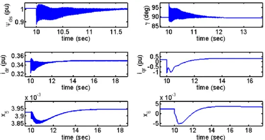
Figure 9. Transient response of stator flux linkage _ds, state variable , rotor currents components (in both axes d and q) and control signals of x5 and x6

Fig.ure 10. Transient response of control signals of x₇ and x₈, rotor angular speed, shaft twist angle, turbine angular speed and q component of grid side filter current

(10)

4-2- Bifurcation Analysis of Grid-Connected WT Based ON DFIG

Numerous considerations manifested saddle-node bifurcation in the bifurcation parameterLe. In fact, when Le

changes from its normal value (0.3pu) to the value of

 

L_e *0.406pu, a simple real eigenvalue approaches zero and

1 0

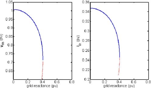
  . Moreover, other eigenvalues have negative real parts. In power systems, grid the venin impedance is not a constant value and changes permanently. Therefore, it is one of the best candidates that its variations and its effect on the wind turbine system should be investigated. Bifurcation diagram of the system is shown in figure 12. In this plot, stretch and dashed lines show stable and unstable equilibrium points, respectively. The border between these two lines is saddle-node bifurcation. Figure 13 shows the system time domain simulation for the state variable i_dr in the case of

 

*

e e

L  L . In this simulation, system is established with L_e 0.4pu and is subjected to a disturbance by a change in

e

L to the value 0.41pu. It can be seen that i_dr increases exponentially after this change.

Figure 12. Bifurcation diagram, state variables ds,idr according to the bifurcation parameter Le.

Figure 13. Time domain simulation of state variable idr after the saddle node bifurcation occurance.

Furthermore, selecting Qsref as a bifurcation parameter reveals that at the value

 

* ref

s 0.373

Q  pu a

complex-conjugate pair of system eigenvalues crosses the imaginary axis and the other eigenvalues remain with the negative real parts. As a result, the DFIG system is exposed to the Hopf bifurcation and got unstable in oscillatory manner if Qsref

passes from

 

Qsref *. Bifurcation diagram is shown in Figure 14. The border between these two lines is Hopf bifurcation.

So, if the reactive power demand of the power network exceed inordinately, wind turbine system gets unstable and state variables become oscillatory. One of the techniques prevent system from this kind of instability is using reactive power sources. In figure 15 two dimension center manifold at the Hopf bifurcation is shown. Figure 16 shows the system time domain simulation for the state variable idr in the case of

 

* ref ref

s s

Q  Q . It can be seen that idr increases oscillatory after

this change. The same happening takes place for the bifurcation parameteridgref. In fact, for this parameter at the value of

 

_ref *

dg 0.353

(11)

Figure 14.Bifurcation diagram, state variable ds according to the bifurcation parameter.

Figure 15. Two dimension center manifold at the Hopf bifurcation.

Figure 16. Time domain simulation of variable idr after the Hopf bifurcation occurance.

In reference [31], it is shown that among all control parameters of WT system based on DFIG, four parameters Vdc

P

K , idqr

P

K , pf P

K and ωr

P

K have the most influence in dynamic performance of the system. In the following the change of these parameters is investigated based on the bifurcation theory and eigenvectors tracking. It is possible to find out the stable region of the controlling parameters. Selecting Vdc

P

K as a bifurcation parameter reveals that at the value

 

Vdc

P 64.721

K   a Hopf bifurcation takes place. Second parameter, idqr P

K imports the continuous algorithm. Minor changes around the



Vdc



P

K is considered and the second parameter idqr P

K is changes until the Hopf bifurcation once more happens. Thus, two-parameter of Hopf bifurcation is derived which is presented in figure 17. Therefore, if controlling parameters Vdc

P

K and idqr P

K settle down on this curve, Hopf bifurcation takes place. Under the curve, all of the real parts of eigenvalues remain in the left side of the imaginary axis and the system is stable. Above the curve, at least two real parts of eigenvalues will have positive values and the system will be unstable. This process can be generalized to three parameters Vdc

P

K , idqr P

K and pf P

(12)

Figure 17. Two-parameter locus of the Hopf bifurcation.

Figure 18. Locus of the Hopf bifurcation parameters.

The variation and variation range of the three parameters are shown in 3-D in terms of geometric location. In this chart, the colors determine the different values of the parameters in trade off mode relatively.

5-

Conclusion

In our analytical simulation, based on related references, a model of a grid-connected wind turbine system presented. This model was schemed as set of differential algebraic equations. The state equations were approached to represent the dynamic mode of the system in time domain simulation, accordance with some external disturbances. Then, bifurcation theory was presented. It was demonstrated that bifurcation theory allows a qualitative assessment and identification of the expected system at different operation points without resorting to time-domain simulations. Stability analysis of DFIG system based on bifurcations theory presented. Our simulation shows a good performance of system model. However, the application of bifurcations theory allows a considerable reduction in the required computation effort. Actually, based on bifurcations theory and applying our simulation the eigenvalues of system were traced. According to the motion of the system eigenvalues due to the change of bifurcation parameters, saddle-node and Hopf bifurcations were extracted. It was shown that behavior of the system is different in comparison to these two methods. In the saddle-node bifurcation, state variables become unstable exponentially but in the Hopf bifurcation they become unstable oscillatory. It was shown that both these two bifurcations take place in the DFIG system.

6-

References

[1] R. Cardenas, R. Pena, S. Alepuz, G. Asher, “Overview of control systems for the operation of DFIGs in wind energy applications”, IEEE Transactions on Industrial Electronics 60 (2013) 2776-2797, doi: 10.1109/iecon.2013.6699116.

(13)

[3] D.C. Gaona, L.M. Goytia, O.A. Lara, “Fault ride-through improvement of DFIG-WT by integrating a two-degree-of-freedom internal model control”, IEEE Transactions on Industrial Electronics 60 (2013) 1133-1145, doi: 10.1109/tie.2012.2216234. [4] Z.S. Zhang, Y.Z. Sun, J. Lin, G.J. Li, “Coordinated frequency regulation by doubly fed induction generator-based wind power

plants”, IET Renewable Power Generation 6 (2012) 38-47, doi: 10.1049/iet-rpg.2010.0208.

[5] A.J.S. Filho, E.R. Filho, “Model-based predictive control applied to the doubly-fed induction generator direct power control”, IEEE Transactions on Sustainable Energy 3 (2012) 398-406, doi:10.1109/tste.2012.2186834.

[6] Y. A. Kuznetsov, Elements of applied bifurcation theory, Second Edition, Springer, 1998, doi: 10.1007/b98848.

[7] S. Wiggins, Introduction to applied nonlinear dynamical systems, Second Edition, Springer, 2003, doi: 10.1007/0-387-21749-5_1.

[8] I. A. Hiskens, “Analysis tools for power systems-contending with nonlinearities”, Proc. IEEE, vol. 83, pp. 1573–1587, Nov. 1995, doi: 10.1109/5.481635.

[9] V. Ajjarapu and B. Lee, “Bifurcation theory and its application to nonlinear dynamical phenomena in an electrical power system”, IEEE Trans. Power Syst., vol. 7, pp. 312–319, Feb. 1992, doi: 10.1109/pica.1991.160594.

[10]H. Wang, E. Abed, and A. M. A. Hamdan, “Bifurcations, Chaos, and crises in voltage collapse of a model power system”, IEEE Trans. Circuits Syst. I: Fund. Theory Appl., vol. 41, no. 2, 294–302, 1994, doi: 10.1016/s0960-0779(02)00072-3.

[11]V. Ajjarapu, and B. Lee, “Bifurcation, Theory and its application to nonlinear dynamical phenomena in an electrical power system”, IEEE Trans. Power Syst., vol. 7, no. 1, pp. 424–431, 1992, doi: 10.1109/pica.1991.160594.

[12]W. Ji, and V. Venkatasubramanian, “Dynamics of a minimal power system: invariant tori and quasi-periodic motions”, IEEE Trans. Circuits Syst. I: Fund. Theory Appl., vol. 42, no. 12, pp. 981–1000, 1995, doi: 10.1109/iscas.1995.521612.

[13]C. A. Canizares, “Voltage stability assessment: concepts, practices and tools”, Tech. rep., IEEE/PES Power System Stability Subcommittee, Final Document, available at http://www.power.uwaterloo.ca, Aug. 2002, doi: 10.4018/978-1-5225-2584-4.ch029.

[14]N. Koppel, and R. B. Washburn, “Chaotic motions in the two-degree-of-freedom swing equations,” IEEE Trans. Circuits Syst., vol. CAS-29, pp. 738–746, Nov. 1982, doi: 10.1109/tcs.1982.1085094.

[15]I. Dobson, and H. D. Chiang, “Toward a theory of voltage collapse in electric power systems,” Syst. Contr. Lett., vol. 13, pp. 253–262, 1989, doi: 10.1109/59.387892.

[16]M. Varghese, F. F.Wu, and P.Varaiya, “Bifurcations associated with subsynchronous resonance,” IEEE Trans. Power Syst., vol. 13, pp. 139–144, Feb. 1998, doi: 10.1036/1097-8542.664550.

[17]C. Kieny, “Application of the bifurcation theory in studying and understanding the global behavior of a ferroresonant electric power circuit”, IEEE Trans. Power Delivery, vol. 6, pp. 866–872, Apr. 1991, doi: 10.1109/61.131146.

[18]H. O. Wang, E. H. Abed, and A. M. A. Hamdan, “Bifurcation, chaos and crisis in voltage collapse of a model power system”,

IEEE Trans. Circuits Syst., vol. 41, no. 3, pp. 294–302, Mar. 1994, doi: 10.1016/s0960-0779(97)00169-0.

[19]S. H. Lee, J. K. Park, and B. H. Lee, “A study on the nonlinear controller to prevent unstable Hopf bifurcation”, in IEEE Power Eng. Soc. Summer Meeting, vol. 2, Jul. 2001, pp. 978–982, doi: 10.1109/pess.2001.970189.

[20]W. D. Rosehart, and C. A. Cañizares, “Bifurcation analysis of various power system models,” Int. J. Elect. Power Energy Syst., vol. 21, no. 3, pp. 171–182, Mar. 1999, doi: 10.1016/s0140-6701(99)91128-1.

[21]C. A. Cañizares, “On bifurcations, voltage collapse and load modeling”, IEEE Trans. Power Syst., vol. 10, pp. 512–522, Feb. 1995, doi: 10.1109/59.373978.

[22]M. A. Pai, P.W. Sauer, and B. C. Lesieutre, “Structural stability in power systems-effect of load models”, IEEE Tran. Power Syst., vol. 10, pp. 609–615, Feb. 1995, doi: 10.1109/apt.1993.686875.

[23]T. K. Vu, and C. C. Liu, “Analysis of tap-changer dynamics and construction of voltage stability regions”, IEEE Trans. Circuits Syst., vol. 36, no. 4, pp. 575–590, Apr. 1989, doi: 10.1109/iscas.1988.15242.

[24]N. Mithulananthan, C. A. Cañizares, J. Reeve, and G. J. Rogers, “Comparison of PSSS, SVC and STATCOM controllers for damping power system oscillations,” IEEE Trans. Power Syst., vol. 18, pp. 786–792, May 2003, doi: 10.1109/tpwrs.2003.811181.

(14)

[26]P. M. Vahdati, A. Kazemi, M. H. Amini, and L. Vanfretti, “Hopf bifurcation control of power system nonlinear dynamics via a dynamic state feedback controller-part I: Theory and Modeling”, IEEE Trans. On Power Systems, Vol. 32, No. 4, pp. 3217-3228, 2017, doi: 10.1109/tpwrs.2016.2633389.

[27]P. M. Vahdati, L. Vanfretti, M. H. Amini, and A. Kazemi, “Hopf bifurcation control of power systems nonlinear dynamics via a dynamic state feedback controller-part II: Performance Evaluation”, IEEE Trans. On Power Systems, Vol. 32, No. 4, pp. 3229-3236, 2017, doi: 10.1109/tpwrs.2017.2679131.

[28]Z. Shuai, Y. Hu, Y. Peng, C. Tu, and Z. J. Shen, “Dynamic stability analysis of synchronverter-dominated microgrid based on bifurcation theory”, IEEE Trans. Trans. On Industrial Electronics, Vol. 64, No. 9, pp. 7467-7477, 2017, doi: 10.1109/tie.2017.2652387.

[29]K. Skandarama, R. C. Mala, and N. Prabhu, “Control of bifurcation in a VSC based STATCOM”, Electrical Power and Energy Systems, vol. 21, pp. 187-195, 2015, doi: 10.2016/j.protcy.2015.10.087.

[30]M. Zamanifar, B. Fani, M. E. H. Golshan, and H. R. Karshenas, “Dynamic modeling and optimal control of DFIG wind energy systems using DFT and NGSA-II”, Electric Power Systems Research, vol. 108, 50-58, 2014, doi: 10.2016/j.epsr.2013.10.021. [31]Y. Tang, P. Ju, H. He, C. Qin, F. Wu, “Optimized control of DFIG-based wind generation using sensitivity analysis and particle

swarm optimization”, IEEE Transactions on Smart Grid vol. 4, pp. 1-12, 2012, doi: 10.1109/pesmg.2013.6672713.