Vol 60, No 2 (2017)

TECHNICAL UNIVERSITY OF CLUJ-NAPOCA

ACTA TECHNICA NAPOCENSIS

Series: Applied Mathematics, Mechanics, and Engineering Vol. 60, Issue II June, 2017

GENERALIZED DELTA RULE WITH ENTROPY ERROR FUNCTION

Javier BILBAO, Imanol BILBAO, Cristina FENISER

Abstract: Machine Learning can refer to a different and various algorithms, based on artificial intelligence, that are able to recognize data patterns through continuous and repeated learning techniques, and we do not have to assume any prior data distribution. In this way, artificial neural networks can provide an effective technology and methodology. Artificial neural networks need a rule, delta rule, in order to learn from the supplied data. In this paper a generalized delta rule with a new error function is presented.

Key words: neural networks, delta rule, error function, cost function.

1. INTRODUCTION

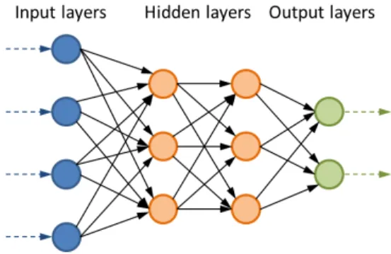
Artificial Neural Networks have proven to be an effective technology in performing tasks in which the human brain provides good results. In addition, thanks to their parallel architecture, they are able to quickly handle the immense amount of data and variables that, today, are available thanks to the wide deployment of mobile technologies and, in general, the so-called Big Data. What’s more, their capacity for adaptation and evolution is also desirable in systems that evolve and develop changing over time.

Feedforward Artificial Neural Networks using classical generalized delta rule have shown ability to classify the data in previously defined clusters, represent the information internally in a way that extracts de data’s features and compresses it, and finally, generalize results to patterns not presented before.

The power of the idea of the generalized delta rule is that even the connections of the network’s internal neurons can adapt to minimize the error between the target and the result of the output neurons. It allows somehow hidden layers’ neurons to create an adequate representation of the information.

2. CONSIDERATIONS ABOUT ERROR FUNCTIONS

For a training data set

(

x t

)

p

r r

, , where tr is the

desired response associated to the xr network

entry data of the pattern p, all the suggested error functions are accumulative and independent respect to their terms, this is, the total error will be a sum of the individual errors. Therefore,

_∑

∀

=

p p total E

E , the total error

is the sum of the error made with each pattern. We will understand total error as a function of the network weights w_ij, and we will try to

locate its minimum value using the gradient descent method.

The fact that

_∑

∀

=

p p total E

E allows us to write

also the partial derivatives as an accumulation for each pattern:

∑

∑

∀ ∀

∂ ∂ = ∂ ∂ = ∂ ∂

p ji p

ji p

p

ji total

w E

w E

w E

(1)

∑

∀ ∂

∂ − = ∂ ∂ − = ∆

p ji p

ji total ji

w E w

E

w (2)

If we name ∆_pw_jisomething that is

proportional to each ji p

w E

∂ ∂

− we are able to write

∑

∀

∆ = ∆

p ji p

ji w

w .

3. CLASSICAL GENERALIZED DELTA RULE

3.1 Used error function

The error function used in [1] is the usual sum-squared error function calculated through all the output layer’s neurons:

(

)

∑

∀

− =

j

pj pj

p t o

E 2

2 1

(3)

pj

t is the j-th component for the desired

output tp

r

. Therefore, it is the desired output for the j-th output neuron when the pattern p is applied.

pj

o is the output obtained in the output

neuron j when xp

r

is presented to the network input layer.

3.2 Initial definitions and used output function

In a purely feedforward network architecture the i layer’s neurons only are connected to the i+1 layer’s neurons. The input layer receives the xr_pdata and transforms it in network signals.

The output layer transmits its signals outside the network. The hidden layers are responsible of finding an appropriate representation of the info to achieve the desired result.

Fig. 1. Feedforward architecture.

In a feedforward architecture each neuron of the network receives signals from the neurons of the previous layer. The effect of these signals is combined in the neuron net total input:

∑

∀

= i

pi ji

pj w o

net (4)

Here the net total input is the linear combination of the previous layer’s neurons output with the corresponding connections weights. The subindex i indicates each neuron of that previous layer and w_ji is the weight of

the connection from the neuron i to the neuron j that’s being analyzed.

As usual in this kind of models, all the neuron’s activation thresholds are θj treated as a weight of a fictitious connection of input 1. In this sense, θj =wj0.

The mathematical development of [1] takes into account that all the neurons in the network have their own generic output function that relates the output of the neuron with the net total input. Therefore,

(

pj

)

j pj f net

o = (5)

The only condition they must fulfill is to be non-decreasing and differentiable.

3.3 Classical generalized delta rule summary

The modification in the weights that should be done after a pattern p is presented is

pi pj ji

pw =ηδ o

∆ (6)

(

pj pj

) (

j pj

)

pj = t −o f' net

δ (7)

For the hidden layers’ neurons:

(

)

∑

∀ = k kj pk pj j

pj f net

δ

w

δ

' (8)

Where k are all the neurons which the neuron j is connected to.

The calculations are divided into two phases. The first is a feedforward propagation of the entry data xr_p through the network, from the

input layer towards output layer. The objective is to generate each neuron’s net total input and each neuron’s output for the known weights. Once net_pj and o_pj have been calculated for all

the neurons the second back propagation phase can be done. Starting in the last layer, with the known tr_p for the used data entry, we calculate

each layers neurons’ δ_pj. Therefore, we calculate δpj for all the neurons of the output

layer, and with all them together we continue calculating the previous layer neurons’ δ_pj just as a linear combination of them. The process continues recursively layer by layer until the input layer is reached.

3.4 Classical generalized delta rule development

Following the general steps provided by [1]

we will calculate ji p w E ∂ ∂

− for each w_ji and try to

write it as the product δpjopi. Thus, we can write: ji pj pj p ji p w net net E w E ∂ ∂ ∂ ∂ = ∂ ∂ (9)

Where netpj is the net total input of the neuron j where the connection w_ji finishes.

From the equation (4) it is easy to follow that pi ji pj o w net = ∂ ∂ (10)

Cause all the other weights act as constants for ∂w_ji.

To compute the other term of (9),

pj pj pj p pj p pj net o o E net E ∂ ∂ ∂ ∂ = ∂ ∂ =

−δ (11)

Where o_pj is the output of the neuron where

the connection wji finishes.

From the equation (5) it follows immediately that

(

pj

)

j pj pj net f net o ' = ∂ ∂ (12)

The first term is more complicated to evaluate. If we suppose that j is a neuron from the output layer, then

(

)

∑

∀ − ∂ ∂ − = ∂ ∂ − k pk pk pj pj p o t o o E ₂ 2 1 (13) pj pj pj p o t o E − = ∂ ∂ − (14)

Cause all the other opkdistinct from opj are

unrelated and act as constants.

If the neuron j is a neuron from the previous layers, we should follow the chain rule, just as indicated in [1]:

pj pk k pk p pj p o net net E o E ∂ ∂ ∂ ∂ − = ∂ ∂ −

∑

∀ (15)

∑

∑

∀ ∀ ∂ ∂ ∂ ∂ − = ∂ ∂ − i pi ji pj k pk p pj p o w o net E o E (16)

∑

∑

∀ ∀ = ∂ ∂ − = ∂ ∂ − k kj pk kj k pk p pj p w w net E o E

δ (17)

4. GENERALIZED DELTA RULE WITH

ENTROPY ERROR FUNCTION

4.1 Desired values and possible output values

and the desired outputs of the network should be in the same range to be interpreted. In classification networks, for example, each output neuron could reflect the probability of a data to belong to a determined predefined class being desirable this property.

We can assure, in accordance with the digital nature of the data collected, that all the target values will be 0 or 1.

On the other hand, we will interpret the output values of each output neuron as the probability of that output to be a 1. To be so it’s neurons output range should be

[ ]

0 . We will ,1 later choose an appropriate output function that fulfils this condition.

4.2 Used error function

The error function is that used in [2] for the logistic regression. For a given pattern the error on each neuron of the output layer is:

(

)

₍

( )

₎

  

= −

−

= −

=

0 1

ln

1 ln

,

pj pj

pj pj pj

pj p

t o

t o o

t

E (18)

This function is a known function in the statistical field making use of the maximum likelihood principle. It’s a concave function where the errors are nearly 0 if the estimation is correct, or near correct, and where the errors tend to infinity if the estimations are incorrect. It takes intermediate values for values that are in an uncertain probability.

If the desired output is tpj =1and the actual output is near 1 the error would be very small. As o_pjtends to 0 the error would increase

slowly, and for values of o_pjnear to 0 the error

would be very big (it tends to infinity as the output tends to 0).

Fig. 2. Error for tpj=1.

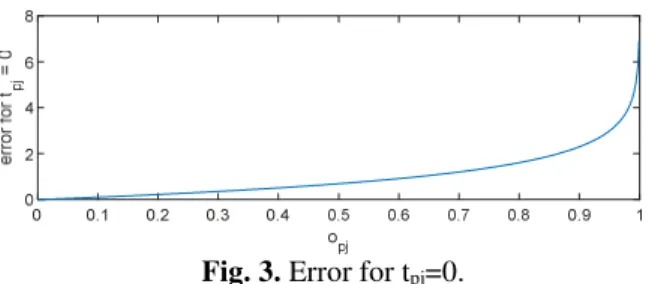
If the desired output is tpj =0and the actual output is near 0 the error would be very small. As o_pjtends to 1 the error would increase

slowly, and for values of o_pjnear to 1 the error

would be very big (it tends to infinity as the output tends to 1).

Fig. 3. Error for tpj=0.

Knowing that the unique values that t_pjcan

have are 0 or 1, the error for the pattern among all the neurons in the output layer may be rewritten as:

( ) (

) (

)

∑

+ − −

− =

j

pj pj

pj pj

p t o t o

E ln 1 ln1 (19)

4.3 Used output function

The used output function is the sigmoidal function. It’s defined by:

(

pj

)

net_pj j

pj

e net

f

o ₋

+ = =

1

1 ₍₂₀₎

It’s a non-decreasing and differentiable function in the range

[ ]

0 that may be ,1 interpreted as the probability of the neuron j to be activated. For low values of netpjit produces outputs that are almost 0. For high values of

pj

net it results in values nearly 1. For values

near to the threshold of activation of the neuron

j

θ it produces a progressive change.

Fig. 4. Sigmoidal output function

(

)

(

)

2

1 ' pj pj net net pj j pj pj e e net f net o − − + = = ∂ ∂ (21)

(

)

pj_pj

pj net net net pj j e e e net f ₋ − − + + = 1 1 1 ' (22)

(

)

_pjpj

pj net net net pj j e e e net f ₋ − − + + − + = 1 1 1 1 1

' (23)

(

)

_       + − + + = _{− −} − pj pj pj net net net pj pj j e e e o net f 1 1 1 1

' (24)

(

)

      + − = ₋ pj net pj pj j e o net f 1 1 1 ' (25)

(

pj

)

pj

(

pj

)

j net o o

f' = 1− (26)

Its derivative is nearly 0 if the output rounds 0 or 1, and has it maximum if net_pjis around

the threshold value.

4.4 Generalized delta rule

We will follow the same steps we have done in the case of the classical generalized delta rule of the section 3.4. We start applying the chain rule introducing the netpj of the neuron j where the connection w_ji finishes:

ji pj pj p ji p w net net E w E ∂ ∂ ∂ ∂ − = ∂ ∂ − (27)

The second term is identical to that of equation (10), so we still can write that

pi ji pj o w net = ∂ ∂ (28)

Just as we did before in (11) and (12) for the recurrent term δ_pj, we begin with its definition and apply the chain rule again, introducing opj,

the output of the neuron where the connection

ji

w finishes:

pj pj pj p pj p pj net o o E net E ∂ ∂ ∂ ∂ − = ∂ ∂ − = δ (29)

(

pj

)

j pj

p

pj f net

o E ' ∂ ∂ − = δ (30)

Fort the output layer neurons the first term of the derivative is a direct application of the partial derivative. It is analogous to that done in (13).

( ) (

) (

)

∑

+ − − ∂ ∂ = ∂ ∂ − k pk pk pk pk pj pj p o t o t o o E 1 ln 1 ln (31)

k is the set of neurons of the output layer. The output layer doesn’t have connections between neurons of the same layer, thus, we know that each opk distinct from opj is

unrelated to ∂o_pj and that acts as a constant in

the derivative. The sum can then be eliminated and write simpler:

( ) ( ) ( )

pj pj pj pj pj pj pj p o t t o o t o E ∂ − ∂ − + ∂ ∂ = ∂ ∂

− ln 1 ln1 (32)

(

pj

)

pj pj pj pj pj pj pj pj p o o o t o t o t o E − − = − − − = ∂ ∂ − 1 1 1 (33)

When both equations (30) and (33) match together the expression obtained is:

pj pj pj p

pj t o

net E − = ∂ ∂ − = δ (34)

It is more simple than that of the classical generalized delta rule in (7) because we have chosen the error function in a way that it’s derivative simplifies with the output function derivative.

For the weights connected to the previous layers’ neurons the procedure is the same we have followed with the classical generalized delta rule in (15), (16) and (17). As the idea is exactly the same they remain unchanged and we still can summarize that for hidden neurons:

(

)

∑

∀ − = k kj pk pj pj

pj o o

δ

w

5. CONCLUSION

Artificial neural networks have taken a new impulse due to different reasons, but mainly because the prominence of Big Data and Machine Learning in the last time, and because their capacity for adaptation and evolution in systems that evolve and develop changing over time. Delta rule is the core of the systems that use artificial neural networks, and although the practical totality of their users take software or libraries of software to use them, it is necessary a mathematical development to create these software.

A generalized delta rule is presented with a new error function. It maintains the same idea of the original rule but with fewer calculations. It’s results can be summarized in three main equations.

The modification in the weights that should be done after a pattern p is presented is

pi pj ji

pw =ηδ o

∆ (36)

The δ_pj for the neurons of the output layer is

(

pj pj

)

pj = t −o

δ (37)

For the hidden layers’ neurons:

(

)

∑

∀

− =

k kj pk pj pj

pj o o

δ

w

δ

1 (38)

6. REFERENCES

[1] Rumelhart, D.E., McClelland, J.L., Paralell Distributed Processing: Explorations in the Microstructure of Cognition, vol. 1,

Cambridge, MA: MIT Press, ISBN 0-262-18120-7, 1986.

[2] Ng, A. CS229 Lecture notes. Machine

Learning. Supervised Learning,

Discriminative Algorithms

http://cs229.stanford.edu/notes/cs229-notes1.pdf

REGULĂ DELTA GENERALIZATĂ CU FUNCȚIE DE EROARE BAZATĂ PE ENTROPIE

Rezumat: Învățarea automată se poate referi la algoritmi diferiți și variați, bazați pe inteligență artificială, capabili să recunoască modele de date prin tehnici de învățare continuăşi repetată, fără a fi nevoie de o distribuție de date anterioară. Astfel, rețelele neuronale artificiale pot contribui la asigurarea unor tehnologii și metodologii eficiente. Rețelele neuronale artificiale au nevoie de o regulă, o regulă Delta, pentru a învăța din datele furnizate. În această lucrare este prezentată o regulă Delta generalizată cu o nouă funcție de eroare.

Javier BILBAO, Professor, University of the Basque Country, Engineering School of Bilbao,

Applied Mathematics Department, [email protected], 0034 94 601 4151.

Imanol BILBAO, PhD Student, University of the Basque Country, Engineering School of Bilbao,

Electrical Engineering Department, [email protected], 0034 94 601 4971, C/ Belostikale 4, 1, 0034 94 415 5896.

Cristina FENISER, Lecturer, Technical University of Cluj Napoca (Romania), Faculty of Machine