Moments of the position of the maximum for GUE
characteristic polynomials and for log-correlated
Gaussian processes.
∗Yan V. Fyodorov
School of Mathematical Sciences, Queen Mary University of London London E1 4NS, United Kingdom
Pierre Le Doussal
CNRS-Laboratoire de Physique Th´eorique de l’Ecole Normale Sup´erieure 24 rue Lhomond, 75231 Paris Cedex-France
Abstract. We study three instances of log-correlated processes on the interval: the logarithm of the Gaussian unitary ensemble (GUE) characteristic polynomial, the Gaussian log-correlated potential in presence of edge charges, and the Fractional Brownian motion with Hurst index H → 0 (fBM0). In previous collaborations we obtained the probability distribution function (PDF) of the value of the global minimum (equivalently maximum) for the first two processes, using the freezing-duality conjecture(FDC). Here we study the PDF of the position of the maximumxm
through its moments. Using replica, this requires calculating moments of the density of eigenvalues in the β-Jacobi ensemble. Using Jack polynomials we obtain an exact and explicit expression for both positive and negative integer moments for arbitrary
β >0 and positive integernin terms of sums over partitions. For positive moments, this expression agrees with a very recent independent derivation by Mezzadri and Reynolds. We check our results against a contour integral formula derived recently by Borodin and Gorin (presented in the Appendix A from these authors). The duality necessary for the FDC to work is proved, and on our expressions, found to correspond to exchange of partitions with their dual. Performing the limitn→0 and to negative Dyson indexβ → −2, we obtain the moments ofxmand give explicit expressions for
the lowest ones. Numerical checks for the GUE polynomials, performed independently by N. Simm, indicate encouraging agreement. Some results are also obtained for moments in Laguerre, Hermite-Gaussian, as well as circular and related ensembles. The correlations of the position and the value of the field at the minimum are also analyzed.
∗
with Appendix A written by Alexei Borodin and Vadim Gorin.
1 Introduction 4
2 Models, method and main results 5
2.1 Results for log-correlated processes . . . 6
2.1.1 GUE characteristic polynomials (GUE-CP): . . . 6
2.1.2 Log-correlated Gaussian random potential (LCGP) with a background potential: . . . 7
2.1.3 Fractional Brownian motion with Hurst index H = 0 (fBm0): . 8 2.2 Moments of the eigenvalue density of the Jacobi ensemble . . . 11
2.3 Replica method and freezing duality conjecture for log-correlated processes 13 3 Acknowledgements 16 4 Calculations within the Replica Method 16 4.1 Connections to the β-Jacobi ensemble . . . 16
4.1.1 GUE characteristic polynomial. . . 16
4.1.2 General scaled model in [0,1]. . . 17
4.1.3 Fractional Brownian motion. . . 17
4.2 Derivation of the moment formula in terms of sums over partitions . . . 19
4.3 Borodin-Gorin contour integral representation of the moments . . . 23
4.3.1 Positive moments. . . 23
4.3.2 Negative moments. . . 24
4.4 duality . . . 24
4.4.1 Statement of the duality on the moments. . . 24
4.4.2 Checking and proving duality for moments. . . 25
4.4.3 Consequence of the duality-invariance: freezing. . . 26
4.5 n = 0 limit of the moments formula . . . 26
4.5.1 Replica limit of sums over partitions. . . 26
4.5.2 Contour integral representation of moments for n = 0. . . 27
4.6 Calculation and results for the first moment. . . 29
4.7 Results for second, third and fourth moments . . . 30
4.7.1 Log-correlated potential with edge charges ¯a,¯b. . . 30
4.7.2 GUE characteristic polynomial. . . 31
4.7.3 Fractional Brownian motion. . . 32
4.8 Results for negative moments . . . 33
5 Other ensembles 36
5.1 General considerations . . . 36
5.2 Moments for the Laguerre ensemble . . . 38
5.2.1 General formula. . . 38
5.2.2 Random statistical mechanics model associated to Laguerre ensemble. . . 38
5.3 Gaussian-Hermite ensemble . . . 39
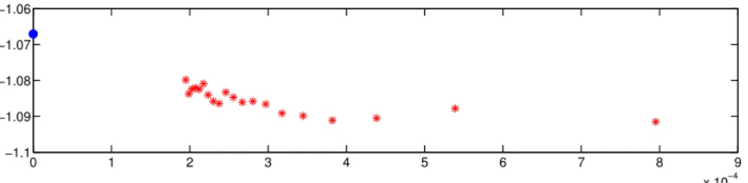
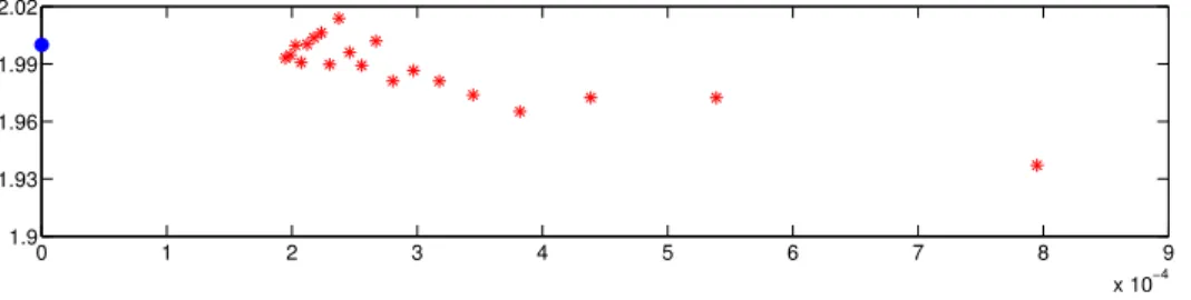
6 Discussion and Conclusions 40 6.1 Numerical verification . . . 40
6.2 Conclusions . . . 41
7 Appendix A: contour integral formulas for Jacobi ensemble 43 8 Appendix B: calculation of contour integrals and more results for moments 49 8.1 Second moment . . . 50
8.2 Third moment . . . 50
8.3 Fourth moment . . . 51
8.4 Second negative moment . . . 52
9 Appendix C: numerical values of higher moments 52 9.1 fBm0 . . . 52
9.2 GUE-CP . . . 53
10 Appendix D: Normalization of Jack polynomials 53 11 Appendix E: Averages over Jacobi measure 54 12 Appendix F: Remark on moment formula 54 13 Appendix G: Distribution of the value of the minimum 55 13.1 Main result . . . 55
13.2 Duality and freezing . . . 57
14 Appendix H: Joint distribution and correlations between value and positions 58 14.1 High temperature phase . . . 59
1. Introduction
Logarithmically correlated Gaussian (LCG) random processes and fields attract growing attention in Mathematical Physics and Probability and play an important role in problems of Statistical Mechanics, Quantum Gravity, Turbulence, Financial Mathematics and Random Matrix Theory, see e.g. recent papers [1], [2] and [3, 4, 5] for introduction and some background references and [6] for earlier review including Condensed Matter applications. A general lattice version of logarithmically correlated Gaussian field is a collection of Gaussian variables VN,x : x ∈ DN attached to the
sites of d−dimensional box DN of side length N (assuming lattice spacing one) and
characterized by the mean zero and the covariance structure
E{VN,x2 }= 2g2logN+f(x), (1)
E{VN,x, VN,y}= 2g2log+
N
|x−y| +ψ(x, y), for x6=y∈DN (2) where ln+(w) = max (lnw,0),g >0 and bothf(x) andψ(x, y) are bounded function far enough from the boundary ofDN. One also can define the continuous versions V(x) of
LCG fields on various domainsD∈Rd which is then necessarily a random generalized
function (”random distribution”), the most famous example being the Gaussian Free field in d= 2, see [7] for a rigorous definition. For d = 1 the one-dimensional versions of LGC processes are known under the name of 1/f noises, see e.g. [8, 9]. They appear frequently in Physics and Engineering sciences, and also are rich and important mathematical objects of interest on their own. Such processes emerge, for example, in constructions of conformally invariant planar random curves [10] and are relevant in random matrix theory and studies of the Riemann zeta-function on the critical line [2]. In particular, the problem of characterizing the distribution of the global maximum
MN = maxx∈DNVN,x of LCG fields and processes (or their continuum analogues)
recently attracted a lot of interest, in physics, see [6, 11, 12, 13, 14, 15] and mathematics, see [16, 17, 18, 2, 19, 20, 21, 22, 23, 24, 25, 26]. The distribution is proved to be given by the Gumbel distribution with random shift [20] and has a universal tail predicted by renormalization group arguments in [6]. The detail of the full distribution are not universal and depend on some details of the behaviour of the covariance (2) for global |x−y| ∼ N scale as well as on the subleading term f(x) in the variance (1). The explicit forms for the maximum distribution were conjectured in a few specific models of 1/f noises [11, 12, 2, 21].
The goal of this paper is to provide some information about the distribution of the
positionof the global minimum
xm = x∈D : V(x) = min y∈DV(y) := Arg minx∈DV(x) (3)
for some examples of 1-dimensional processes with logarithmic correlations, though depending on applications, one can be interested instead in a maximum. Statistical properties of the value and position for maxima and minima are obviously trivially related in cases when V(x) = −V(x)in law.
Our first example is the modulus of the characteristic polynomial of a random GUE matrix over the interval [−1,1] of the spectral parameter. As is well-known, in the limit of large sizes of the matrix the logarithm of that modulus is very intimately related to 1/f noises [1, 2, 21, 27, 28]. In that example the interesting quantity is obviously the statistics of the maximum, with minimum value being trivially zero at every characteristic root of the matrix. The second example is a general two-parameter variant of a log-correlated process on the interval with, in the language of Coulomb gases, endpoint charges, introduced and studied in [12]. That case may include a non-random (logarithmic)background potential V0(x), so that for the sum V0(x) +V(x) we have
min[V0(x) +V(x)] =−max[−V0(x) +V(x)], in law
Our last example is a regularized version of the fractional Brownian motion with zero Hurst index, which is a bona fide (nonstationary) 1d LCG process [1]. Here statistics of maxima and minima are trivially related by symmetry in law.
2. Models, method and main results
We now define the three models to be considered. Although we did not yet succeed in obtaining the full probability distribution function (PDF),P(xm), of the position of
the global minimum xm, we derive formulae for all positive integer moments of xm in
terms of sums over partitions. In this section we present explicit values for some low moments ofxm, more results can be found in the remainder of the paper.
As is clear from [12] there is an intimate relation between statistics of extrema in log-correlated fields on an interval and the β-Jacobi ensemble of random matrices [29, 30]. In the course of our calculation we present methods to calculate the moments of the eigenvalue density of the Jacobi ensemble. In this section we provide a very explicit formula for these moments derived in remainder of the paper. In particular our result is in agreement with recent results by Mezzadri and Reynolds [31]. We check our results against a contour integral representation derived recently by Borodin and Gorin (presented in the Appendix A from these authors) which, remarkably, also allows to calculate negative moments.
Finally we sketch the replica method and the application of the freezing-duality conjecture to extract the moments ofxm from the moments of the Jacobi ensemble.
2.1. Results for log-correlated processes
2.1.1. GUE characteristic polynomials (GUE-CP):
Our first prediction is for the lowest moments of the position of the globalmaximum
for the the modulus of the characteristic polynomial pN(x) = det(xI − H) of the
HermitianN ×N matrix H sampled with the probability weight
P(H)∝exp(−2NTr(H2)) (4)
known as the Gaussian Unitary Ensemble (or GUE)[32, 33, 34]. Here the variance is chosen to ensure that asymptotically forN → ∞, the limiting mean density of the GUE eigenvalues is given by the Wigner semicircle lawρ(x) = (2/π)√1−x2 supported in the intervalx ∈ [−1,1]. Hence the object we want to study is log|pN(x)| =Piln|x−λi|
where the λi are the eigenvalues of the GUE matrix H. To study its fluctuations it
turns out to be more convenient to subtract its mean. This leads to the following
Prediction 1. Define φN(x) = 2 log|pN(x)| −2E(log|pN(x)|)and consider the random
variable
x(mN):=Arg maxx∈[−1,1]φN(x) (5)
Then the lowest even integer moments of this random variable have the values
lim N→∞E n x(mN)2o = 13 49, Nlim→∞E n x(mN)4o = 20 147 (6)
whereas the odd integer moments vanish by symmetry.
In particular, the kurtosis of the distribution of x(mN) in the large-N limit is given
by lim N→∞ E h x(mN) i4 E h x(mN) i22 −3 =−541 507 ≈ −1.067. . . (7)
To make a contact between |pN(x)| and the LCG processes we refer to the paper
[1]. That work revealed that the natural large-N limit of φN(x) is given by the random
Chebyshev-Fourier series F(x) =−2 ∞ X n=1 1 √ nanTn(x), x∈(−1,1), (8)
with Tn(x) = cos(narccos(x)) being Chebyshev polynomials and real an being
covariance structure associated with the generalized processF(x) is given by an integral operator with kernel
E{F(x)F(y)}= 4 ∞ X n=1 1 nTn(x)Tn(y) = −2 log(2|x−y|), (9)
as long asx6=y. Such a limiting processF(x) is an example of an aperiodic 1/f-noise. Note however that the series (8) is formal and diverges with probability one. In fact it should be understood as a random generalized function (distribution). Though there is no sense in discussing the maxima and its position for generalized functions, the problem is well-defined for the logmod of the characteristic polynomial log|pN(x)| for
any finite N. One therefore needs to find a tool to utilize its asymptotically Gaussian nature evident in (8). It turns out that the latter is encapsulated in the following asymptotic formula due to Krasovsky [35]1 which will be central for our considerations:
E k Y j=1 |pN(xj)|2δj ! = k Y j=1 C(δj)(1−x2j) δ2 j/2(N/2)δj2e(2x2j−1−2 log(2))δjN (10) ×exph− X 1≤i<j≤k 2δiδj log|2(xi−xj)| i 1 +O logN N where C(δ) := 22δ2G(δ+1)2
G(2δ+1), with G(z) being the Barnes G-function. In particular, differentiating with respect toδ, we deduce that
E(2 log|pN(x)|) =N(2x2−1−2 log(2)) +C0(0) +O(log(N)/N). (11)
The formula (10) suggests that, apart from the factors C(δj) which as we shall
see play no role in our calculations, the faithful description of 2 log|pN(xj)| is that
of the regularized GLC process with covariance (9), the position-dependent variance 2 lnN + ln√1−x2−ln 2
and the position-dependent mean N(2x2 −1− 2 log(2)). We find it convenient to subtract the mean value and concentrate on the centered GLC
φN(x) in Prediction 1. As to the position-dependent logarithmic variance (stemming
from the factors (1−x2j)δj2/2 in (10)) we shall see that it does play a very essential role
in statistics of the position of global maximum for|pN(x)| via giving rise to nontrivial
”edge charges” in the corresponding Jacobi ensemble. This observation corroborates with the earlier mentioned fact that the subleading position-dependent term f(x) in the variance of the LCG, see (1), may modify the extreme value statistics.
2.1.2. Log-correlated Gaussian random potential (LCGP) with a background potential:
1 See also earlier works [36, 37] where such formula was anticipated and proved for positive integerδ
An interesting question is to study the position of the minimum for the sum of a LCG random potential and of a determistic background potential, i.e:
xm = Argminx∈D V(x) +V0(x)
(12) Here we obtain results whenDis an interval, sayx∈[0,1]. The LCG random potential has correlations:
E{V(x)V(x0)}=C(x−x0) , lim
→0C(x) = −2 ln|x| |x|>0 (13) andC(0) = 2 ln(1/) where is a small scale regularization. The background potential
is of the special logarithmic form:
V0(x) = −¯alnx−¯bln(1−x) (14)
which we will often refer to, following the Coulomb gas language, as ”edge charges” at the boundary. We mainly focus on the case of repelling charges, ¯a,¯b >0, although both the model, and some of our results, extend to some range of attractive charges. Some properties of this model, such as the PDF of the value of the total potential at the minimum, were studied in [12]. Here we obtain, for the two lowest moments ofxm
Prediction 2. E{xm} − 1 2 = ¯ a−¯b 2(¯a+ ¯b+ 4) (15) Ex2m −(E{xm})2 = (¯a+ 2)(¯b+ 2)(2¯a+ 2¯b+ 9) (¯a+ ¯b+ 4)2(¯a+ ¯b+ 5)2 (16) Note that for the background potential V0(x) alone, i.e. in the absence of disorder, and for ¯a,¯b >0, the minimum for the background potentialV0(x) alone is atx0m = ¯a+¯a¯b, that is x0 m − 1 2 = ¯ a−¯b
2(¯a+¯b). Hence the disorder brings the minumum closer in average to the midpoint x= 12.
2.1.3. Fractional Brownian motion with Hurst indexH = 0 (fBm0):
The fractional Brownian motion introduced by Kolmogorov in 1940 and
rediscovered in the seminal work by Mandelbrot & van Ness [38] is defined as the Gaussian process with zero mean and with the covariance structure:
E{BH(x1)BH(x2)}= σH2 2 |x1| 2H +|x2|2H − |x1−x2|2H , (17)
where 0 < H < 1 and σ2H = Var{BH(1)}. The utility of these long-ranged correlated
processes is related to the properties of being self-similar and having stationary
In particular, for H = 1/2 the fBm B1/2(t) ≡ B(t) is the usual Brownian motion (Wiener process). Note however that naively putting H = 0 in (17) does not yield a well-defined process. Nevertheless we will see below that the limitH →0 for fractional Brownian motion can be properly defined after appropriate regularization and yields a Gaussian process with logarithmic correlations.
Consider a family of Gaussian processes depending on two parameters: 0≤H <1 and a regularization η >0 and given explicitly by the integral representation [1]
BH(η)(x) = √1 2 Z ∞ 0 e−ηs s1/2+H n e−ixs −1Bc(ds)/2 + eixs−1Bc(ds)/2 o . (18)
HereBc(s) = BR(s)+iBI(s), withBR(s) andBI(s) being two independent copies of the
Wiener processB(t) (the standard Brownian motion) so thatB(dt) is the corresponding white noise measure, E{B(dt)}= 0 andE{B(dt)B(dt0)}=δ(t−t0)dtdt0.
The regularized process {B(Hη)(x) : x ∈ R} is Gaussian, has zero mean and is characterized by the covariance structure
E n BH(η)(x1)B (η) H (x2) o =φ(Hη)(x1) +φ (η) H (x2)−φ (η) H (x1−x2), (19) where φ(Hη)(x) = 1 2 Z ∞ 0 e−2ηs s1+2H (1−cos (xs))ds (20) = 1 4HΓ(1−2H) (4η2+x2)Hcos 2Harctan x 2η −(2η)2H . (21) It is easy to verify that for any 0 < H < 1 one has limη→0B
(η)
H (x) = BH(x) which is
precisely the fBm defined in (17).
As has been already mentioned the limit η → 0 for H = 0 does not yield any well-defined process. At the same time taking the limit H→0 at fixed η gives
lim H→0φ (η) H (x) = 1 4log x2+ 4η2 4η2 , (22)
ensuring that for anyη >0 the limit ofBH(η)(x) asH →0 yields a well-defined Gaussian process{B(0η)(x) :x∈R} with stationary increments and with the increment structure function depending logarithmically on the time separation:
E h B0(η)(x1)−B (η) 0 (x2) i2 = 1 2log |x1−x2|2+ 4η2 4η2 . (23)
We consider B0(η)(x) as the most natural extension of the standard fBm to the case of zero Hurst indexH = 0. We will frequently refer to this process as fBm0. The process is regularized at scales|x1−x2|<2η.
It is also worth pointing out that there exists an intimate relation betweenB0(η)(x) and the behaviour of the (incrementsof) GUE characteristic polynomials, though at a different, so-called ”mesoscopic” spectral scales [1], negligible in comparision with the interval [−1,1]. The mesoscopic intervals are defined as those typically containing in the limit N → ∞ a number of eigenvalues growing with N, but representing still a vanishingly small fraction of the total number N of all eigenvalues. In other words, fBM0 describes behaviour of the (logarithm of) theratioof the moduli of characteristic polynomial at mesoscopic difference in spectral parameter. More precisely, B0(η)(x) is , in a suitable sense, given byN → ∞ limit of the following object:
WN(x) = 1 2π −log det " x dN I−H 2 + η 2 4d2 N # + log det H2+ η 2 4d2 N ! (24)
whereH is anN×N random GUE matrix, parameterη >0 is a regularisation ensuring that the logarithms are well defined for real x and dN specifies the asymptotic scale of
the spectral axis of H as N → ∞ and is chosen to be mesoscopic 1 dN N (say, dN =Nγ with 0< γ <1).
Applying our methods of dealing with LCG to fbM0 yields the following predictions for a few lowest moments of the position of the global minimum for the processB0(η)(x) in the interval 0, L:
Prediction 3. Define V(x) = 2B0(η)(x) and for η > 0 and L >0 consider the random variable
ym(η, L) :=
1
LArg minx∈[0,L]V(x) (25)
Then the lowest even integer moments of this random variable have the values
lim η→0E [ym(η, L)]2 = 17 50, limη→0E [ym(η, L)]4 = 311 1470 (26)
whereas the odd integer moments can be found from the identities
lim η→0E ( ym(η, L)− 1 2 2k+1) = 0, k = 0,1,2, . . . (27)
One should point out an interesting difference in application of our method to this case, concerning the value of the minimum Vm = minx∈[0,1]V(x), which seems to be a direct consequence of non-stationarity of the fBm0. Since the process is constrained to the value V(0) = 2B0(η)(0) = 0 at zero, Vm is necessarily negative or zero, at variance
with the other cases studied here. As discussed in Appendix G, this implies that the method of analytical continuation in n of Ref. [12], which works nicely for the other cases, fails to predict the PDF of Vm for the fBm0, and requires modifications which
the moments of xm, which enjoy a nice and simple analytical continuation to n = 0.
As we checked numerically up to large n, these moments pass the standard tests (i.e. positivity of Hankel matrices) for existence of a positive associated PDF. Conditional
moments however, i.e. conditioned to an atypically high value of Vm, would need a
more careful study, beyond the scope of this paper.
2.2. Moments of the eigenvalue density of the Jacobi ensemble
As mentioned above the statistics of extrema in log-correlated fields on an interval relate to the β-Jacobi ensemble of random matrices. We denote y = (y1, . . . , yn) the
set of eigenvalues, with yi ∈ [0,1], i = 1, . . . , n. The model can be defined [29, 30] by
the joint distribution of eigenvalues2 PJ(y)dy= 1 Zn n Y i=1 dyiyai(1−yi)b|∆(y)|2κ , ∆(y) = Y 1≤i<j≤n (yi−yj) (28)
where the normalization constant, Zn, is the famous Selberg integral [39] for which an
explicit formula exists for any positive integern
Zn=Sln(κ, a, b) := Z [0,1]n |∆(y)|2κ n Y i=1 yia(1−yi)bdyi (29) = n−1 Y j=0 Γ (a+ 1 +κj) Γ (b+ 1 +κj) Γ (1 +κ(j+ 1)) Γ (a+b+ 2 +κ(n+j−1)) Γ (1 +κ)
In [12] we analytically continued this formula to complexnwhich allowed to obtain the probability distribution of the height of the global minimum of the process (see also [40],[41],[42],[43]). In the present paper we advance this analysis much further in order to extract the statistics of the position of the global minimum. As we will show this requires to obtain some exact formula for the moments of the eigenvalue density for the β-Jacobi ensemble for arbitrary positive integer n. Furthermore these should be explicit enough to allow for a continuation ton = 0.
Let us define the average value < f(y) >J of any function f(y) over the Jacobi
density by the relation
< f(y)>J:= [Sln(κ, a, b)]−1 Z [0,1]n f(y)|∆(y)|2κ n Y i=1 yia(1−yi)bdyi (30)
In particular for any positive integern the mean density of eigenvalues is defined as:
ρJ(y) =< 1 n n X i=1 δ(yi−y)>J=< δ(y1−y)>J (31) 2 Note that we use 2κfor the Dyson index instead ofβto avoid confusion with the inverse temperature,
whereδ is the Dirac distribution. The moments studied here are then defined as:
Mk(J) =
Z 1
0
dyykρJ(y) =< y1k>J (32)
The problem of calculating these moments, for the β-Jacobi ensemble, has been already addressed in the theoretical physics and mathematical literature, motivated by various applications. In full generality it turns out to be a hard problem, and only limited results were available. One method is based on recursion on the order of the moment, as outlined in the chapter 17 of Mehta’s book [33] and used in [44, 45] in the context of conductance distribution in chaotic transport through mesoscopic cavities. In that approach higher moments calculations become technically unsurmountable. Another approach using Schuhr functions was developed and gave very explicit results for these and other moments for β = 1,2 [46] (see also related work in [47] and [48]).
More recently, an interesting contour integral representation for those moments was proved by Borodin and Gorin, but remained unpublished. It is described in the Appendix A to the present paper, provided by these authors. It allows a systematic calculation of the moments, including negative ones. However evaluating these integrals becomes again a challenge for higher moments.
In the present paper we give an explicit expression for all integer moments, positive and negative, of the eigenvalue density for the β-Jacobi ensemble, based on a different approach, in terms of sums over partitions.
Let us further denote λ = (λ1 ≥ λ2 ≥ ..≥ λ`(λ)) a partition of length `(λ) of the integer k ≥ 0, with λi strictly positive integers such that |λ| =P`i=1(λ)λi =k. Then we
obtain * 1 n n X j=1 yjk + J = X λ,|λ|=k Aλa+λ , * 1 n n X j=1 yj−k + J = X λ,|λ|=k Aλa−λ (33)
where the sum is over all partitions ofk, and
Aλ = k(λ1−1)! (κ(`(λ)−1) + 1)λ1 `(λ) Y i=2 (κ(1−i))λi (κ(`(λ)−i) + 1)λi Y 1≤i<j≤`(λ) κ(j−i) +λi−λj κ(j−i) (34) × 1 n `(λ) Y i=1 (κ(n−i+ 1))λi (κ(`(λ)−i+ 1))λi Y 1≤i<j≤`(λ) (κ(j −i+ 1))λi−λj (κ(j−i−1) + 1)λi−λj
in terms of the Pochhammer symbol (x)n =x(x+ 1)..(x+n−1) = Γ(x+n)/Γ(x), with
for positive moments
a+λ = `(λ) Y i=1 (a+ 1 +κ(n−i))λi (a+b+ 2 +κ(2n−i−1))λi (35)
while for negative moments a−λ = `(λ) Y i=1 (a+ 1 +κ(i−1))−λi (a+b+ 2 +κ(n+i−2))−λi (36) This result as it stands was derived for n, k ∈ N and κ > 0, and in range of values of
a, bsuch that these moments exist. Later however we will study analytic continuations in these parameters.
For positive moments, this very explicit formula is equivalent to a result by Mezzadri and Reynolds, which appeared in [31] during the course of the present work. Our independent derivation is relatively straightforward and will be given below for both positive and negative moments.
One can check on the above expressions (33)-(34), that in the limitκ→0 partitions contribute as ∼ κ`(λ)−1, hence only the single partition λ = (k) with a single row contributes, leading to the trivial limit for the moments:
* 1 n n X j=1 yjk + J,κ=0 = (a+ 1)k (a+b+ 2)k (37) here fork of either sign, as expected, since in that limit the Jacobi measures decouples PJ(y) = Qn i=1P 0(y i) where P0(y) = Γ(a+b+2) Γ(a+1)Γ(b+1)y
a(1−y)b. Other general properties
of the moments, such as identity of moments of y and of 1 −y for a = b, are less straightforward to see on the above formula, and are explicitly checked below for low moments.
2.3. Replica method and freezing duality conjecture for log-correlated processes
Our method of addressing statistics related to the globalminimumof random functions (which can be trivially adapted for the global maximum with obvious modifications) is inspired by statistical mechanics of disordered systems. Namely, we look at any random functionV(x) defined in an intervalD∈Rof the real axis as a one-dimensional random potential, with x playing the role of spatial coordinate. To that end we introduce for any β > 0 and any positive β−independent weight function µ(x) > 0 the associated Boltzmann-Gibbs-like equilibrium measure by
pβ(x) = 1 Zβ µ(x)e−βV(x)≡ 1 Zβ Z D δ(x−x1)e−βV(x1)µ(x1)dx1, (38) where we have defined the associated normalization function (the ”partition function”)
Zβ = Z
D
e−βV(x)µ(x)dx (39)
According to the basic principles of statistical mechanics in the limit of zero temperature β → ∞ the Boltzmann-Gibbs measure must be dominated by the minimum of the random potential Vm = minx∈D V(x) achieved at the point xm ∈ D.
The latter is randomly fluctuating from one realization of the potential to another. The probability density for the position of the minimum is defined as P(x) = δ(x−xm)
where from now on we use the bar to denote the expectation with respect to random process (”potential disorder”) realizations:
(. . .)≡E{(. . .)}
This leads to the fundamental relation
P(x) = lim
β→∞pβ(x) (40)
Therefore, calculating P(x) amounts to (i) performing the disorder average of the Boltzmann-Gibbs measure (38) and (ii) evaluating its zero-temperature limit. The second step is highly non-trivial, due to a phase transition occuring at some finite value β = βc. In our previous work on decaying Burgers turbulence [49], which
turns out to be a limiting case of the present problem (see Section 5.3), we have already succeeded in implementing that program. Following the same strategy, the step (i) is done using the replica method, a powerful (albeit not yet mathematically rigorous) heuristic method of theoretical physics of disordered systems. It amounts to representing Zβ−1 = limn→0Zβn−1 which after assuming integer n > 1 results in the
formal identity pβ(x) = lim n→0pβ,n(x) (41) where pβ,n(x) =µ(x)e−βV(x)Zβn−1 = Z x1∈D ... Z xn∈D e−βPn =1V(xi) δ(x−x 1) n Y i=1 µ(xi)dxi (42)
Note that pβ,n(x) is not a probability distribution for general n, but becomes one for n= 0.
In the next section we will show how to calculate the moments Mk(β) = R
Dpβ,n(x)x
kdx for positive integer k and any integer value n > 0 in the high
temperature phase of the modelβ < βc. Note that by a trivial rescaling of the potential
one always can ensure βc = 1, setting g = 1 in (1), and we assume such a rescaling
henceforth. In the rangeβ <1 the formulae we obtain for the moments turn out to be easy to continue to n = 0. This yields the integer moments of the probability density
pβ(x) in that phase. There still however remains the task of finding a way to continue
those expressions to β > 1 in order to compute the limit β → ∞ and extract the information about the Argmin distributionP(x). To perform the continuation, we rely
on the freezing transition scenario for logarithmically correlated random landscapes. The background idea goes back to [6] and was advanced further in [11] leading to explicit predictions. In [12] it was discovered that the duality property appears to play a crucial role, leading to the freezing-duality conjecture (FDC), which was further utilized in [49, 9, 13, 2, 21, 14]. In brief, the FDC predicts a phase transition at the critical valueβ = 1 and amounts to the following principle:
Thermodynamic quantities which for β <1 areduality-invariant functions of the
inverse temperature β, that is remain invariant under the transformation β →β−1,
”freeze” in the low temperature phase, that is retain for all β >1 the value they
acquired at the point of self-duality β = 1.
Here, on our explicit formula, we will indeed be able to verify that every integer momentMk(β) =
R
Dpβ,n=0(x)x
kdxof the probability densityp
β(x) isduality-invariant
in the above sense, and hence can be continued to β > 1 using the FDC, yielding the moments of the position of the global minimum. Another way of proof is based on the powerful contour integral representation for the moments of Jacobi ensemble of random matrices provided by Borodin and Gorin. We thus conjecture that not only all moments, but the whole disorder averaged Gibbs measurepβ(x) freezes atβ = 1, hence
that the PDF of the position of the minimum is determined as P(x) = lim
β→1pβ(x) (43)
similar to the conjecture in [49] in our study of the Burgers equation.
Although the FDC scenario is not yet proven mathematically in full generality and has a status of a conjecture supported by physical arguments and available numerics, recently a few nontrivial aspects of freezing were verified within rigorous probabilistic analysis, see e.g. [22, 50, 23, 20] for progress in that direction 3. However the role of duality has not yet been verified rigorously. Interesting connections to duality in Liouville and conformal field theory [51] remain to be clarified.
In the rest of the paper we give a detailed derivation of the outlined steps of our procedure and an analysis of the results.
3 In [6, 11, 12] we predicted the freezing of the generating functiong
β(y) := exp(−eβyzβ), wherezβis
a regularized version of the partition sumZβ. It was proved in [23] (see corollary 2.3) in a more general
and rigorous setting. It tells about the free energyfβ =−β−1lnzβ and thevalue of the minimum
f∞. Indeed, by construction 1−gβ(y) is the cumulative distribution function of the random variable
defined asyβ :=fβ−β−1G whereG is a unit Gumbell random variable, independent fromfβ. The
3. Acknowledgements
The authors are very grateful to Nick Simm for kindly providing numerical data on argmax of GUE, as well as to Alexei Borodin and Vadim Gorin for bringing their methods to our attention, for writing the Appendix A in the present paper, and for indicating relevant references to us. We would like to warmly thank the anonymous referee for suggesting to use formulas (80,81) for obtaining an explicit expression for the negative moments, Alberto Rosso for a lively discussions at the early stage of the project, and Dima Savin for guiding us to the literature on the moments of Jacobi density. We also thank F. Mezzadri and A. Reynolds for informing us on their moment formulae prior to publication. Kind hospitality of the Newton Institute, Cambridge during the program ”Random Geometry” as well as of the Simon Center for Geometry and Physics in Stony Brook, where this research was completed, is acknowledged with thanks. YF was supported by EPSRC grants EP/J002763/1 “Insights into Disordered Landscapes via Random Matrix Theory and Statistical Mechanics” and EP/N009436/1 ”The many faces of random characteristic polynomials”. PLD was supported by PSL grant ANR-10-IDEX-0001- 02-PSL.
4. Calculations within the Replica Method
Our goal in this section is to develop the method of evaluating the required disorder average and calculating the resulting integrals explicitly in some range of inverse temperaturesβ for a few instances of the log-correlated random potentials V(x).
4.1. Connections to the β-Jacobi ensemble
4.1.1. GUE characteristic polynomial. In that case we will follow the related earlier
study in [21] and use the family of weight factors µ(x) = ρ(x)q on the interval x ∈ [−1,1], with ρ(x) = π2√1−x2 and parameter q > 0. Such a choice of the weight is justified a posteriori by the possibility to find within this family a duality-invariant expression for the moments in the high-temperature phase which is central for our method to work. Since here we are interested in the maximum of the characteristic polynomial we will define the potential V(x) = −φN(x) where φN(x), defined in
Prediction 1, is not strictly a Gaussian field. Nevertheless due to the Krasovsky formula (10) we can write asymptotically in the limit of large N 1
e−βPn a=1V(xa) =eβPna=1φN(xa) = n Y a=1 |pN(xa)|2βe−2β Pn a=1ln|pN(xa)| (44) 'An n Y a=1 (1−x2a)β2/2Y a<b |xa−xb|−2β 2 (45)
with An= [C(β)(N/2)β 2
e−βC0(0)2−β2(n−1)
]n.
4.1.2. General scaled model in [0,1]. It is easy to see that by proper rescaling the
evaluation of the functionpβ,n(x) from (42) amounts in the case of both characteristic
GUE polynomials and the LCGP process to evaluating particular cases of the following multiple integral defined on the interval [0,1]:
pβ,a,b,n(y) = Z 1 0 .. Z 1 0 n Y i=1 dyiyai(1−yi)b Y 1≤i<j≤j≤n 1 |yi−yj|2β 2 δ(y−y1) (46)
which is formally the (un-normalized) density of eigenvalues of the β-Jacobi ensemble (28), i.e. pβ,a,b,n(y) =ZnρJ(y), however with a negative value of the parameterκ=−β2.
In particular the normalisation factor Zn is the Selberg integral (29). Note that both
integrals are well defined forβ2 <1 and positive integern. They can also be defined for largerβ, upon introducing an implicit small scale cutoff which modifies the expressions for|yi−yj|< . However we will use only the high temperature regime and will continue
analytically our moment formula ton = 0 andβ = 1.
These integrals are associated to the statistical mechanics of a random energy model generated by a LCG field in the interval [0,1] in presence of boundary charges of strengtha and b. More precisely, they appear in the study of the continuum partition function introduced in [12]
Zβ =β 2Z 1
0
dyya(1−y)be−βV(y) (47)
where the correlator ofV(x) was defined in (13). Hereaandbare the two parameters of the model and the factorβ2
ensures that the integer momentsZn
β are -independent in
the high temperature regime. There, these moments Zn
β =Zn are given by the Selberg
integral (29). Several aspects of this model, such as freezing, duality and obtaining the PDF of the value of the minimum, were analyzed in [12]. Here we will focus instead on the calculation of the moments of the position y. In each realization of the random potential V they are defined as
< yk >β,a,b= R1 0 dyy kya(1−y)be−βV(y) R1 0 dyya(1−y)be −βV(y) (48)
and we will be interested in calculating their disorder averages < yk > β,a,b.
4.1.3. Fractional Brownian motion. For our fBm0 example we take the weight function
µ(x) = 1 in (38), (39) on the interval x ∈[0, L], and use the rescaled fBm with H = 0 as the random potential: V(x) = 2gB0(η)(x). Exploiting the Gaussian nature of fBm0
we can easily perform the required average using (19) which yields e−2βgPn i=1B (η) 0 (xi) =e2(βg) 2 Pn i=1 h B(0η)(xi) i2 +2Pn i<jB (η) 0 (xi)B0(η)(xj) (49) =en(2βg)2Pni=1φ (η) 0 (xi)−(2βg)2Pni<jφ (η) 0 (xi−xj) (50)
Further using the definitions (22)-(23) we arrive at
e−2βgPn i=1B (η) 0 (xi) = n Y i=1 x2i + 4η2 4η2 a/2 n Y i<j (xi−xj)2+ 4η2 4η2 −γ (51) a= 2nγ , γ =g2β2 (52)
Assuming that all xi >0 we can write in the limit of vanishing regularization η →0: e−2βgPn i=1B (η) 0 (xi) ≈(2η)n(γ(n−1)−a) n Y i=1 xai n Y i<j |xi−xj|−2γ (53)
For convenience we will use the particular valueg = 1 ensuring a posteriorithe critical temperature value βc= 1.
It is easy to see how our three examples can be studied within the framework of the model (46):
• GUE characteristic polynomial. We define x= 1−2y, , with y∈[0,1] and
pβ,n(x)dx =Cnpβ,a,a,n(y)dy , a = q+β2 2 (54) Cn= [( 2 π) qC(β)Nβ2 e−βC0(0)21+q−2β2(n−1)]n (55) • LCGP plus a background potential on interval [0,1], defined in (13) and (14). One
sees that this model is obtained by choosing a=β¯a and b=β¯b. • fBm0: we definex=Ly, with y∈[0,1] and:
pβ,n(x)dx =Ln(n+1)γ+npβ,a=2nβ2,b=0,n(y)dy (56)
Although the explicit form of the density ρJ(y) of the β-Jacobi ensemble is not
known in a closed form for finiten, the formulae (33)-(34) displayed in the introduction provide an explicit expression for its integer moments
< yk >β,a,b,n:= 1 Zn Z 1 0 dyykpβ,a,b,n(y) (57)
for positive integersk, n andβ2 <0. The collection of indicesβ, a, b, nis now replacing the indexJ, and some of them may be omitted below when no confusion is possible.
We will now derive the formulae (33)-(34) using methods based on Jack polynomials. In a second stage we will continue them analytically to arbitrary n,
including n = 0, and to 0 < β2 ≤ 1, to obtain moments for the random model of interest as: < yk > β,a,b = lim n→0< y k > β,a,b,n (58)
4.2. Derivation of the moment formula in terms of sums over partitions
To calculate the moments, we now consider one of the most distinguished bases of symmetric polynomials, the Jack polynomials, named after Henry Jack. They play a central role for our study because their average with respect to the β-Jacobi measure is explicitly known, due to Kadell [52] (see below). As discussed in the book [53] (see reprint of the original article) Jack introduced a special set of symmetric polynomials ofn variablesy:= (y1, . . . , yn) indexed by integer partitions λand dependent on a real
parameter α. He called them Z(λ), which in modern notations are denoted as Jλ(α)(y) following I. Macdonald who greatly developed the theory of such and related objects in the book [54]. Another important source of information is Stanley’s paper [55]. In what follows we use notations and conventions from [54] and [55]. 4
Let us recall the definition of a partition λ = (λ1 ≥ λ2 ≥ .. ≥ λ`(λ)) > 0) of the integerk, of length`(λ), withλi strictly positive integers such that|λ|:=
P`(λ)
i=1 λi =k.
It can be written as
λ={(i, j)∈Z2; 1≤i≤`(λ),1≤j ≤λi} (59)
from which one usually draw the Young diagram representing the partition λ, as a collection of unit area square boxes in the plane, centered at coordinates i along the (descending, southbound) vertical, and j along the (eastbound) horizontal. The dual (or conjugate) λ0 of λ is the partition whose Young diagram is the transpose of λ, i.e. reflected along the (descending) diagonal i=j. Hence λ0i is the number of j such that
λj ≥ i. If s = (i, j) stands for a square in the Young diagram, one defines the ”arm
length”aλ(s) =λi−j which is equal to the number of squares to the east of square s
and the ”leg length”lλ(s) =λ0j−i as the number of squares to the south of the square s. One then defines the product
c(λ, α, t) :=Y s∈λ (αaλ(s) +lλ(s) +t) = `(λ) Y i=1 λi Y j=1 (α(λi−j) +λ0j−i+t) (60)
which will be used later on5.
Given a partition λ, one defines, in the theory of symmetric functions, the monomial symmetric functions mλ(y), over n variables y = {yr}, r = 1, , n as 4 Note that other papers use different conventions. The reader is advised to check the conventions
with care. 5 Note thatc(λ, α,1) =Q s∈λh λ ∗(s) andc(λ, α, α) =Qs∈λh ∗
mλ(y) = P σ Qn r=1y λi
σ(r) where the summation is over all non-equivalent permutations of the variables. For example, given a partition (211) of k = 4, m(211)(y) = y12y2y3 +
y1y22y3+y1y2y32. Another useful set of symmetric functions, of obvious importance for the calculation of moments, are the power-sums:
pλ(y) = `(λ) Y i=1 n X r=1 yλi r
which form a basis of the ring of symmetric functions.
Define the following scalar product, which depends on a real parameterα as
< pλ, pµ >=δλµzλα`(λ) , zλ = 1q12q2..q1!q2!.. (61) where qi = qi(λ) is the number of rows in λ whose length are equal to i. Here and
below we suppress the arguments of all symmetric polynomials except when explicitly needed, for examplepλ(y)→pλ. The Jack functions J
(α)
λ obey the following properties
(i) orthogonality with respect to the above scalar product (ii) fixed coefficient of highest degree in the monomial basis6
< Jλ(α), Jµ(α) >=c(λ, α,1)c(λ, α, α)δλµ (62) Jλ(α)=c(λ, α,1)mλ+
X
ν<λ
uλνmν (63)
We can go from the basis of power sums to the Jack polynomial basis by the following linear transformations:
Jλ(α)=X ν θλν(α)pν , pν = X λ γνλ(α)Jλ(α) (64)
where the coefficients are in general complicated. Note that the k-th moment that we are interested in is precisely the Jacobi ensemble average
< n X
r=1
yrk >J=< p(k)(y)>J (65)
where (k) denotes the partition with only one row of length k. Hence we need only the coefficient γλ
ν=(k). As we now show one can express this coefficient in terms of θ
λ ν=(k). Indeed, one can write in two ways the following scalar product, first as
< Jλ(α), pµ>= X ν θνλ(α)< pν, pµ>=θλµ(α)zµα`(µ) (66) and also as < Jλ(α), pµ>= X τ γµτ(α)< Jλ(α), Jτ(α) >=γµλ(α)c(λ, α,1)c(λ, α, α) (67)
Hence, comparing we obtain
γµλ(α) = θ
λ
µ(α)zµα`(µ)
c(λ, α,1)c(λ, α, α) (68)
valid for arbitrary partitions µand λ, which we apply to µ= (k). Now it turns out thatθλ(k)(α) is known to to be equal to:
θ(λk)(α) = Y
s−{1,1}
(αa0λ(s)−l0λ(s)) (69) if |λ| = k and zero otherwise, (see p 383 Ex. 1 (b) in [54] and (19) in [56]), where
a0λ(s) =j−1 and l0λ(s) = i−1 are respectively called the co-arm and co-leg lengths of the partitionλ, and the product does not include the box s = (1,1).
Positive moments: this leads to the explicit result for the positive k-th moment in
terms of an average of the Jack polynomial associated to the partition (k):
< n X r=1 yrk >J=< p(k)(y)>J= X λ,|λ|=k γ(λk)(α)< Jλ(α)(y)>J (70) γ(λk)(α) = kα c(λ, α,1)c(λ, α, α) Y s−{1,1} (αa0λ(s)−lλ0(s)) (71) (see Appendix F for an alternative rewriting of this formula).
The problem therefore amounts to evaluating the Jacobi average ofJλ(α)(y). Such averages where evaluated for a general partition λ, for a differently normalized set of Jack polynomials, denoted by Macdonald as Pλ(α)(y), related to the Jλ(α)(y) as follows
Jλ(α)(y) = c(λ, α,1)Pλ(α)(y) (72)
Namely, as was conjectured by Macdonald in [54], and proved by Kadell [52], there exists a closed form expression for Pλ(α)(y) integrated with the (unnormalized) Jacobi density over the hypercube y∈[0,1]n with the correspondence
α= 1/κ (73) It is given by Z [0,1]n Pλ(1/κ)(y)|∆(y)|2κ n Y i=1 yia(1−yi)bdyi (74) =n!vλ(κ) n Y i=1 Γ (λi+a+ 1 +κ(n−i)) Γ (b+ 1 +κ(n−i)) Γ (λi+a+b+ 2 +κ(2n−i−1)) where vλ(κ) = Y 1≤i<j≤n Γ (λi−λj+κ(j−i+ 1)) Γ (λi−λj +κ(j−i)) (75)
For the empty partition λ= (0) we have P(0)(1/κ)(y) = 1 and the above integral reduces to the Selberg integral (29).
Recalling the definition of the Jacobi ensemble average (30) and taking the ratio of (74) to (29), we obtain the average of theP(1/κ)(y) polynomial and from it, the average ofJ(1/κ)(y). The calculation is detailed in the Appendix E and the final result is simple and explicit for arbitrary partitionλ
D Jλ1/κ(y)E J =κ−|λ| `(λ) Y i=1 (a+ 1 +κ(n−i))λi (a+b+ 2 +κ(2n−i−1))λi (κ(n−i+ 1))λi (76)
Putting together Eqs. (70-71) and (76) we obtain the k-th moment as
* 1 n n X r=1 yrk + J = X λ,|λ|=k kα c(λ, α,1)c(λ, α, α) Y s−{1,1} (αa0λ(s)−lλ0(s)) (77) × 1 nκk `(λ) Y i=1 (a+ 1 +κ(n−i))λi (a+b+ 2 +κ(2n−i−1))λi (κ(n−i+ 1))λi (78)
whereαshould be replaced by 1/κaccording to (73). Using the explicit expressions for the normalization constants (211) and (212) in Appendix D and the above definitions of the co-arm and co-leg, one obtains the formula (33), (34), (35), for the positive moments given in Section 2.2. 7.
We have also used:
Y s−{1,1} (αa0λ(s)−l0λ(s)) =αk−1 `(λ) Y i=1 λi 0 Y j=1 (j −1−κ(i−1)) =αk−1(λ1−1)! `(λ) Y i=2 (−κ(i−1))λi (79) where the prime indicates that i=j = 1 is excluded from the product.
Equivalently, we can rewrite the expression (77) for the moments in a ”geometric” form which involves only products over boxes in the Young diagrams, see (91)-(92) below.
Negative moments: Negative moments can be obtained by applying (70) to the
inverse variable, here before averaging (withk ≥0)
n X r=1 y−rk = X λ,|λ|=k γ(λk)(α)Jλ(α)(1 y) (80) where we denote (y1) ≡ (y1 1, .. 1
yn). We now use the following relation between Jack
polynomials, for n≥`(λ) Pλ(α)(1 y) =y −l 1 ..y −l n P (α) (ln−λ)+(y) (81)
7 Note that a textbook treatment of the material discussed in this section is given in [30]. The formula
for the positive moments does not appear there explicitly, but can be recovered by integrating (12.145) using (12.143).
see [30] p. 643, wherel is (a priori) any integer l≥λ1 and one denotes
(ln−λ)+ ={l, ..., l−λ1, .., l−λ`(λ)} (82)
the partition of length n. Using (72) in (80), inserting (81), using again (72), one can now average over the Jacobi measure as follows
* n X r=1 yr−k + J = X λ,|λ|=k γ(λk)(α) c(λ, α,1) c((ln−λ)+, α,1) D J((lαn)−λ)+(y) E J,a→a−l Sln(κ, a−l, b) Sln(κ, a, b) (83) where the average on the right is over a shifted Jacobi measure with parametera−l, b, κ
to account for the prefactor in (81). For the same reason the ratio of Selberg integrals appear, since it is the normalization of the Jacobi measure. We can now use the explicit expressions (29) and (76). One finds, after a tedious calculation, similar in spirit to the one described above for the positive moments, the formula (33), (34) for the negative moments given in Section 2.2 with
a−λ = `(λ) Y i=1 (a−l+ 1 +κ(i−1))l−λi (a−l+b+ 2 +κ(n+i−2))l−λi (a−l+b+ 2 +κ(n+i−2))l (a−l+ 1 +κ(i−1))l (84) where a priori l is an integer sufficiently large. In practice we found that for generic values ofκ the final result is independent of the choice of l (for each partition), hence we chose l= 0 which leads to the simplest expression (36) given in in Section 2.2.
We now discuss an interesting alternative and useful representation for the (positive and negative) integer moments in terms of contour integrals.
4.3. Borodin-Gorin contour integral representation of the moments
4.3.1. Positive moments. Recently Borodin and Gorin proved integral representations
for the moments of the Jacobiβ-ensemble. We refer to the Appendix A for derivation and present here a summary of results in our notation. They call these moments
1
NMk(θ, N, M, α) and the correspondence from their four parameters to ours is:
θ → −β2 N →n θα−1→a , θ(M −N + 1)−1→b (85)
which leads to the correspondence
< yk >β,a,b,n= 1 nMk(−β 2, n, n−1− 1 +b β2 ,− 1 +a β2 ) (86)
Translated in our parameters their moment formula for positive integern reads:
< yk >β,a,b,n= 1 nβ2 Z k Y i=1 dui 2iπ Y 1≤i<j≤k uj −ui (uj−ui+β2)(uj−ui+ 1) (87) × Y 1≤i+1<j≤k (uj−ui+ 1 +β2) k Y i=1 ui+β2 ui+β2(1−n) × ui−1−a ui−2−a−b−β2(1−n) (88)
which must be supplemented with the conditions, let us call them C1: |u1| |u2| |u3|.. |uk| and C2: all the contours enclose the singularities at ui =−(1−n)b2 and
not at ui = 2 +a+b+β2(1−n). These conditions imply that one can first perform
the integral on u1 and only around the pole u1 = −(1−n)β2 and then iteratively on
u2, u3, ..and so on.
We will investigate below the properties of this representation in the context of the models we study here.
4.3.2. Negative moments. Remarkably, Borodin and Gorin also proved a contour
integral formula for negative moments, whenever they exist. In our notations, for
k≥1, it reads < y−k >β,a,b,n= −1 nβ2 Z k Y i=1 dui 2iπ Y 1≤i<j≤k uj−ui (uj−ui−β2)(uj−ui−1) × Y 1≤i+1<j≤k (uj−ui−1−β2) k Y i=1 ui−nβ2 ui ×ui−1−a−b−β 2(1−n) ui−a (89) which must be supplemented with the conditions, (i) C1: |u1| |u2| |u3|.. |uk|
and (ii)C2: all the contours enclose the singularities at 0 and not ata.
4.4. duality
Let us now discuss an important property of these moment, the duality.
4.4.1. Statement of the duality on the moments. For clarity let us first recall the
property of duality-invariance unveiled in [12]. Consider first a thermodynamic quantity
Oβ obtained in the replica formalism in the limit n = 0. This quantity is said to be
duality-invariant if it is well defined in the high temperature region β < 1 and its temperature dependence is given by a function f(β) which is known analytically, and satifies f(β0 = 1/β) = f(β). The simplest example of such quantities is the mean free energy for Gaussian log-correlated models for whichf(x) =x+ 1/x. More complicated examples are presented in [12], see e.g. (13)-(14) there. Note that it does not imply anything on the behaviour of Oβ for β > 1, hence it is strictly a property of the high
temperature phase. However the property of duality invariance is not restricted to the replica limitn = 0. In [12] by considering the generating functions for the moments of the partition function, one notices that duality invariance can be extended to finite n
In the present model, there are more parameters and we can formulate the duality-invariance property for the moments as follows:
Duality-invariance property:
< yk >β,a,b,n=< yk >β0,a0,b0,n0 β0 = 1/β n0 =β2n a0 =a/β2 b0 =b/β2 (90)
which, again, should be understood in the sense of analytical continuation (i.e. it does not provide a mapping from the high to low temperature region as discussed above).
4.4.2. Checking and proving duality for moments. The duality property (90) can be
checked on the explicit formula (33)- (35), derived in this paper. Here we focus on positive moments, but similar considerations hold for negative ones, when they exist. To see it explicitly it is convenient to rewrite that formula in a ”geometric” form involving only products over boxes in the Young diagrams, as
< yk>β,a,b,n:= * 1 n n X r=1 yrk + J κ=−β2 = X λ,|λ|=k lim →0 k n Y s=(i,j)∈λ Bλ(s) κ=−β2 (91) where Bλ(s) = (j−1−(i−1)κ+)(a+κ(n−i) +j)(κ(n−i+ 1) +j−1) (aλ(s) +lλ(s)κ+ 1)(aλ(s) +lλ(s)κ+κ)(a+b+ 1 +κ(2n−i−1) +j) (92) wherehas been introduced only to remove box (1,1) from one of the products and the limit →0 is trivial. For application to the present purpose we need to set κ=−β2.
The duality is easy to check on that formula and corresponds to the exchange of the partitionλ with its dual λ0. Indeed it is easy to check that
Bλ(s)|κ=−β2 β,n,a,b = Bλ0(s0)|κ=−β02 β0,n0,a0,b0 (93)
where s0 = (j, i) is the box in the dual diagram conjugate to s = (i, j), which implies that arm lengths and leg lengths are also exchanged under duality. A similar observation over duality-invariant sum over partitions was reported very recently in [14] for a related problem, about the value at the minimum of a log-correlated field.
Another proof of the duality invariance property for the moments was provided in the recent work Borodin and Gorin (BG). They proved that these moments are rational functions of their four arguments, and that the corresponding analytical continuation in these arguments satisfies an invariance property, which is equivalent to the above duality-invariance (90) under the correspondence (86).
4.4.3. Consequence of the duality-invariance: freezing. Let us now examine the implications of the relation (90) for the three examples studied in this paper, showing that a freezing transition at β = 1 is expected in all cases.
For the GUE problem a = b = q+2β2 and one finds that the duality invariance in terms of the parameter q can be written as:
q0 = 1 + q−1
β2 (94)
The choice q = 1 thus ensures duality-invariance of the moments for arbitrary β < 1 and again implies freezing atβ = 1.
More generally, starting from Jacobi ensemble measure (28) one can ask how to choose a and b so that the model exhibits the duality-invariance. Consider two (otherwise arbitrary) duality-invariant functions of β, ¯a(β) and ¯b(β), i.e. satisfying ¯
a(1/β) = ¯a(β) and ¯b(1/β) = ¯b(β), and choose:
a=β¯a(β) , b=β¯b(β) (95)
Then the moments are self-dual. Our second example Eq. (13) and (14) of a log-correlated potential in presence of a background potential, corresponds to the case of temperature independent constants ¯aand ¯b and its moments are thus duality-invariant. Finally, for the fBm0 the parameter a = 2nβ2 and b = 0. One checks from (90) that the fBm0 satisfies duality invariance for arbitraryn. In the replica limitn= 0 we must set a=b = 0, which is a self-dual point, hence for this model the moments obey the following duality-invariance forβ <1
< yk >β=< yk >1/β (96)
so that according to the FDC, one should expect them to exhibit freezing atβ = 1.
4.5. n = 0 limit of the moments formula
The moment formula obtained above, as well as their contour integral representation are explicit enough to allow for analytic continuation to n= 0.
4.5.1. Replica limit of sums over partitions.
Consider the formula (33)-(34) inserting κ = −β2. The limit n → 0 is straightforward, except for one of the factors in the second line for which we use:
(−β2n)λ1 =−β
2n(1−β2n)
λ1−1 'n→0 −β
2n(λ
1−1)! (97)
This leads to the following formula for the disorder averages of the moments (48) of the general scaled disordered statistical mechanics model (47)
< yk > β,a,b =
X
λ,|λ|=r
with Cλ1 =−β2k[(λ1−1)!]2 `(λ) Y i=2 [(β2(i−1))λi] 2 `(λ) Y i=1 (a+ 1 +β2i) λi (a+b+ 2 +β2(i+ 1)) λi (99) × Y 1≤i<j≤`(λ) λi−λj+β2(i−j) β2(i−j) Cλ2 = `(λ) Y i=1 1 (1 +β2(i−`(λ))) λi(β 2(i−`(λ)−1)) λi Y 1≤i<j≤`(λ) (β2(i−j−1))λi−λj (1 +β2(i+ 1−j)) λi−λj (100) This formula is valid in the higher temperature phase of the model,β <1, where all the factors are clearly finite and non-zero. We will study explicitly below a few moments and their temperature dependence. Note that in the limit β → 0 one recovers the moments (37) (i.e. with the weightP0(y)).
The moments of the position of the scaled minimum of the potential as discussed above are recovered in the zero temperature limit β= +∞of the statistical mechanics model. According to the FDC (see section) these moments are equal to their value at the freezing transition β = 1. Hence they can be obtained by taking as limits
(ym)k = lim β→1−< y
k>
β,a,b (101)
of the above expression (98)-(100). However in this expression one easily sees that the factor Cλ
2 has poles for β = 1, while C1λ is regular and has a finite limit. Examination of low moments, detailed below, show massive cancellations of these poles leading to a well defined finite limit. As shown below, using the contour integral representation, this limit is indeed finite for any moment. Note that the poles in the limit β → 1 are also present for n > 0, so consideration of finite n does not help to handle these cancellations.
The formula (101) together with formula (98)-(100) thus gives arbitrary positive integer moments of the position of the global minimum of the log-correlated process and as such is a main result of our paper. They can be used to generate these moments to a very high degree on the computer.
4.5.2. Contour integral representation of moments for n = 0.
(i)positive moments. To take the limit n= 0 in the contour integral formula (87)
we rewrite 1 nβ2 k Y i=1 ui+β2 ui+β2(1−n) = 1 nβ2 k Y i=1 (1 + nβ 2 ui+β2(1−n) ) = 1 nβ2 + k X i=1 1 ui+β2 +O(n) Inserting the first term in the contour integral gives zero. Next, it is easy to see that only the pole in u1 gives non zero residue. Hence we can insert only this term in the
integral (87), where we can now safely taken= 0 leading to the following representation for the disorder average:
< yk > β,a,b= Z k Y i=1 dui 2iπ Y 1≤i<j≤k uj −ui (uj−ui+β2)(uj −ui+ 1) (102) × Y 1≤i+1<j≤k (uj−ui+ 1 +β2) 1 u1 × k Y i=1 ui−1−a−β2 ui−2−a−b−2β2 (103) where we have shiftedui →ui−β2 for convenience. This again must be supplemented
with the condition (i) C1 : |u1| |u2| |u3|.. |up| and (ii) C2: all the contours enclose the singularities atu1 = 0 but not atui = 2+a+b+2β2. In practice the contours
will run (and close) in the negative half plane Re(ui) < 0 and pick up residues from
poles on the negative real line. We note that one needs the condition 2 +a+b+ 2β2 >0 which, fora=b is precisely the one found in [12] corresponding to a binding transition to the edge (fora <−1−β2). We will thus assume that the condition is fulfilled, which is the case for all three examples considered here.
The limit β → 1 can be performed explicitly leading to a contour integral representation for the positive integer moments of the position of the global extremum of the log-correlated field
yk m = Z k Y i=1 dui 2iπ Y 1≤i<j≤k uj−ui (uj −ui+ 1)2 Y 1≤i+1<j≤k (uj −ui + 2) 1 u1 k Y i=1 ui−2−a ui−4−a−b (104) with the same contour conditionsC1 and C2. This formula should thus be equivalent to our main result (101)-(98)-(100), which we have checked for a few low order moments.
(i) negative moments. The same manipulation as above in the limit n → 0 gives
the disorder averaged moments fork ≥1:
< y−k > β,a,b= Z k Y i=1 dui 2iπ Y 1≤i<j≤k uj −ui (uj −ui−β2)(uj−ui−1) × Y 1≤i+1<j≤k (uj−ui−1−β2) 1 u1 × k Y i=1 ui−1−a−b−β2 ui−a (105) provided these moment exist. Taking again the limit β → 1 one obtains the negative integer moments of the position of the global extremum of the log-correlated field as
y−k m = Z k Y i=1 dui 2iπ Y 1≤i<j≤k uj −ui (uj −ui−1)2 Y 1≤i+1<j≤k (uj −ui−2) 1 u1 × k Y i=1 ui−2−a−b ui−a (106)
fork positive integer, provided they exist. In both integrals the contours obey the two conditions (i) C1: |u1| |u2| |u3|.. |uk| and (ii) C2: all the contours enclose the singularities at 0 and not at a. At present there is no equivalent formula in terms of sums over partitions, hence the above formula is an important result of the paper.
We now turn to explicit study of the low moments
4.6. Calculation and results for the first moment.
Let us illustrate the calculation using the contour integral (87) on the simplest example of the first moment k= 1
< y >β,a,b,n = 1 nβ2 Z du 1 2iπ u1+β2 u1+β2(1−n) u1−1−a u1−2−a−b−β2(1−n) = 1 +a−β 2(n−1) 2 +a+b−2β2(n−1) (107)
which is equal to the residue atu1 =−(1−n)β2. In terms of partitions only the partition
λ= (1) contributes, so it is easy to see on (33)-(34), and even more immediate on (91)-(92) [usingi = j = 1, aλ =`λ = 0], that it reproduces (71). One can explicitly verify
on this result that the first moment is invariant by the duality transformation (90). The n= 0 limit yields the disorder averaged first moment
< y >β,a,b=
1 +a+β2
2 +a+b+ 2β2 (108)
For the symmetric situation a = b, which is the case both for the fBm a =b = 0 and for the GUE characteristic polynomiala=b= 1+2β2 the first moment is thus simply
< y >β =
1
2 (109)
In the second example of the LCGP with edge charges one obtains:
< y >β =
1 + ¯aβ+β2
2 + (¯a+ ¯b)β+ 2β2 (110)
The duality-freezing conjecture then leads to the the first moment of the position of the minimum ym = 2 + ¯a 4 + ¯a+ ¯b , ym− 1 2 = ¯ a−¯b 2(¯a+ ¯b+ 4) (111)
which is Eq. (15) in Prediction 2.
These results can be compared to the first moment in absence of the random potential and at finite inverse temperatureβ, i.e. from the measure P0(y)|
a=βa,b¯ =β¯b < y >P0 − 1 2 = β(¯a−¯b) 2(2 +β(¯a+ ¯b)) (112)
which reproduces the absolute minimumy0
m = ¯a/(¯a+ ¯b) in the absence of disorder for β = +∞. Comparing with (111) shows that even at the freezing temperature β = 1, disorder brings the average position closer to the midpoint y= 12.
4.7. Results for second, third and fourth moments
The calculation of the second moment by the contour integral method is relatively simple, and sketched in the Appendix B section 8.1 for n = 0. It leads to the disorder average:
< y2 >
β,a,b =
(a+β2+ 1) (β2(4a+ 2b+ 9) + (a+ 2)(a+b+ 2) + 4β4)
(a+ 2β2+b+ 2) (a+ 2β2+b+ 3) (a+ 3β2+b+ 2) (113) This expression is also easily recovered from the sum (33)-(34), or (91)-(92) involving now the two partitions (2) and (1,1). For β = 0 it reproduces (37), i.e. the trivial average with respect to the weightP0(y)∼ya(1−y)b. The expression (113) is
duality-invariant and we expect that it freezes atβ = 1 leading to the predictions for the second moment of the position of the extremum.
Let us now detail the results for each example separately, including moments up tok = 4 when space permits, more detailed derivations and results being displayed in the Appendix B.
4.7.1. Log-correlated potential with edge charges ¯a,¯b. The second moment of the
position of the global minimum is obtained from above as 8
y2
m =
(¯a+ 2)(¯a(¯a+ ¯b+ 8) + 4¯b+ 17)
(¯a+ ¯b+ 4)(¯a+ ¯b+ 5)2 (114) This leads to the variance (16) in Prediction 2, replacing there x → y. Expressions for higher moments for general ¯a,¯b are too bulky to present here, and we only display the third moment in (192) and the skewness in (193).
Two special cases are of interest:
(i)only one edge charge, at y = 0: One sets ¯b = 0. Let us give here the skewness
in that case Sk := (ym−ym) 3 (ym−ym)2 3 2 =−√¯a(¯a+ 5)(¯a(7¯a+ 68) + 164) 2√¯a+ 2(¯a+ 6)2(2¯a+ 9)3/2 (115) which is negative. It can be compared with the skewness associated to the measure ∼y¯a, which is Sk0 =− 2¯a√¯a+ 3 √ ¯ a+ 1(¯a+ 4) (116)
8 One sees on this expression that binding to the edge y
m → 0+ (resp. ym → 1−) occurs when
One finds thatSk decreases from 0 to −7/4 as ¯a increases, while Sk0 decreases from 0 to−2, hence they are quite distinct.
(ii) symmetric case ¯a= ¯b. The variance is obtained as:
y2
m−ym2 =
4¯a+ 9
4(2¯a+ 5)2 (117)
where we recall, ym = 12, and we checked explicity that the moment formulae lead to ym− 1 2 3 = 0 (118)
as expected by symmetryy→1−y. The fourth moment and kurtosis are obtained as
y4 m = 4a5+ 84a4+ 663a3+ 2488a2+ 4478a+ 3110 4(a+ 3)(2a+ 5)2(2a+ 7)2 (119) Ku =−2 (8a 5+ 248a4+ 2054a3+ 7328a2+ 12053a+ 7523) (a+ 3)(2a+ 7)2(4a+ 9)2 (120) The kurtosis can be compared to the one of the measureya¯(1−y)¯a which is:
κ0 =− 6
5 + 2a (121)
Note that when ¯a increases, Ku→ −1/4 while Ku0 →0.
4.7.2. GUE characteristic polynomial. For the GUE-CP we must insert a=b= 1+2β2,
in (92). The second moment for the associated statistical mechanics model in the high temperature phase β < 1, and for the position of the global minimum (obtained by settingβ = 1) are then found to be:
< y2 > β = 15β4+ 32β2+ 15 4 (3β2+ 4) (4β2+ 3) , y 2 m = 31 98 (122)
For completeness the expression at finite n is given in (191). In the original variable
x∈[−1,1], i.e. the support of the semi-circle, using x = 1−2y and the result for the first moment we obtain:
< x2 > β = 3 + 7β2+ 3β4 (4 + 3β2)(3 + 4β2) , x 2 m = 13 49 = 0.265306.. (123) where we expect now the PDF of the position of the maximum, P(x), to be centered and symmetric around x= 0 (which was checked explicitly up to fifth moment).
We give directly the fourth moment of the position of the maximum (see 8.3 for finite temperature expressions)
y4 m = 401 2352 , x 4 m = 20 147 = 0.136054.. (124)