Learning to Detect Objects in Images via a Sparse,
Part-Based Representation
Shivani Agarwal, Aatif Awan and Dan Roth,
Member, IEEE Computer Society
Abstract— We study the problem of detecting objects instill, grayscale images. Our primary focus is development of a learning-based approach to the problem, that makes use of a sparse, part-based representation. A vocabulary of distinctive object parts is automatically constructed from a set of sample images of the object class of interest; im-ages are then represented using parts from this vocabulary, together with spatial relations observed among the parts. Based on this representation, a learning algorithm is used to automatically learn to detect instances of the object class in new images. The approach can be applied to any object with distinguishable parts in a relatively fixed spatial con-figuration; it is evaluated here on difficult sets of real-world images containing side views of cars, and is seen to success-fully detect objects in varying conditions amidst background clutter and mild occlusion. In evaluating object detection approaches, several important methodological issues arise that have not been satisfactorily addressed in previous work. A secondary focus of this paper is to highlight these issues and to develop rigorous evaluation standards for the object detection problem. A critical evaluation of our approach under the proposed standards is presented.
Keywords— Object detection, image representation, ma-chine learning, evaluation/methodology.
I. Introduction
T
HE development of methods for automatic detection of objects in images has been a central challenge in computer vision and pattern analysis research. The main difficulty in developing a reliable object detection approach arises from the wide range of variations in images of objects belonging to the same object class. Different objects be-longing to the same category often have large variations in appearance. In addition, the same object can appear vastly different under different viewing conditions, such as those resulting from changes in lighting, viewpoint and imaging techniques [1]. A successful object detection approach must therefore be able to represent images in a manner that ren-ders them invariant to such intra-class variations, but at the same time distinguishes images of the object class from all other images.In this paper, we present an approach for learning to detect objects in images using a sparse, part-based repre-sentation. Part-based representations for object detection form the basis for a number of theories of biological vision [2], [3], [4], [5], and have also been shown to offer
advan-S. Agarwal, A. Awan and D. Roth are with the Department of Com-puter Science, University of Illinois at Urbana-Champaign, Urbana, IL 61801, USA. Email: {sagarwal,mawan,danr}@uiuc.edu
A preliminary version of this work was presented at the Seventh European Conference on Computer Vision in May 2002.
c
2004 IEEE. Personal use of this material is permitted. However, permission to reprint/republish this material for advertising or pro-motional purposes or for creating new collective works for resale or redistribution to servers or lists, or to reuse any copyrighted compo-nent of this work in other works must be obtained from the IEEE.
tages in computational approaches [6]. In the approach presented here, the part-based representation is acquired automatically from a set of sample images of the object class of interest, thus capturing the variability in part ap-pearances across the sample set. A classifier is then trained, using machine learning techniques, to distinguish between object and non-object images based on this representation; this learning stage further captures the variation in the part structure of object images across the training set. As shown in our experiments, the resulting algorithm is able to accurately detect objects in complex natural scenes.
This paper also discusses several methodological issues that arise when evaluating object detection approaches. For an area that is increasingly becoming an active fo-cus of research, it is necessary to have standardized and meaningful methods for evaluating and comparing differ-ent approaches. We iddiffer-entify some important issues in this regard that have not been satisfactorily addressed in pre-vious work, and propose possible solutions to them. A. Related Work
A number of different approaches to object detection that use some form of learning have been proposed in the past. In most such approaches, images are represented us-ing some set of features, and a learnus-ing method is then used to identify regions in the feature space that correspond to the object class of interest. There has been considerable variety in both the types of features used and the learning methods applied; we briefly mention some of the main ap-proaches that have been proposed, and then discuss some recent methods that are most closely related to ours.
Image features used in learning-based approaches to ob-ject detection have included raw pixel intensities [7], [8], [9], features obtained via global image transformations [10], [11], and local features such as edge fragments [12], [13], rectangle features [14], Gabor filter based representations [15] and wavelet features [16]. On the learning side, meth-ods for classifying the feature space have ranged from sim-ple nearest neighbor schemes to more comsim-plex approaches such as neural networks [8], convolutional neural networks [17], probabilistic methods [11], [18] and linear or higher degree polynomial classifiers [13], [16].
In our approach, the features are designed to be object parts that are rich in information content and are specific to the object class of interest. A part-based representation was used in [6], in which separate classifiers are used to de-tect heads, arms and legs of people in an image, and a final classifier is then used to decide whether a person is present. However, the approach in [6] requires the object parts to be
manually defined and separated for training the individual part classifiers. In order to build a system that is easily ex-tensible to deal with different objects, it is important that the part selection procedure be automated. One approach in this direction is developed in [19], [20], in which a large set of candidate parts is extracted from a set of sample im-ages of the object class of interest, an explicit measure of information content is computed for each such candidate, and the candidates found to have the highest information content are then used as features. This framework is ap-pealing in that it naturally allows for parts of different sizes and resolutions. However, the computational demands are high; indeed, as discussed in [20], after a few parts are cho-sen automatically, manual intervention is needed to guide the search for further parts so as to keep the computational costs reasonable. Our method for automatically selecting information-rich parts builds on an efficient technique de-scribed in [21], in which interest points are used to collect distinctive parts. Unlike [21], however, our approach does not assume any probabilistic model over the parts; instead, a discriminative classifier is directly learned over the parts that are collected. In addition, the model learned in [21] re-lies on a small number of fixed parts, making it potentially sensitive to large variations across images. By learning a classifier over a large feature space, we are able to learn a more expressive model that is robust to such variations.
In order to learn to identify regions in the feature space corresponding to the object class of interest, we make use of a feature-efficient learning algorithm that has been used in similar tasks in [13], [22]. However, [13], [22] use a pixel-based representation, whereas in our approach, images are represented using a higher-level, more sparse representa-tion. This has implications both in terms of detection accuracy and robustness, and in terms of computational efficiency: the sparse representation of the image allows us to perform operations (such as computing relations) that would be prohibitive in a pixel-based representation. B. Problem Specification
We assume some object class of interest. Our goal is to develop a system which, given an image as input, returns as output a list of locations (and, if applicable, corresponding scales) at which instances of the object class are detected in the image. It is important to note that this problem is distinct from (and more challenging than) the commonly studied problem of simply deciding whether or not an input image contains an instance of the object class; the latter problem requires only a ‘yes/no’ output without necessar-ily localizing objects, and is therefore really an instance of an image classification problem rather than a detection problem. Evaluation criteria for the detection problem are discussed later in the paper.
C. Overview of the Approach
Our approach for learning to detect objects consists broadly of four stages; these are outlined briefly below: (i) Vocabulary Construction
The first stage consists of building a “vocabulary” of parts that can be used to represent objects in the target class. This is done automatically by using an interest operator to extract information-rich patches from sample images of the object class of interest. Similar patches thus obtained are grouped together and treated as a single part.
(ii) Image Representation
Input images are represented in terms of parts from the vocabulary obtained in the first stage. This requires deter-mining which parts from the vocabulary are present in an image; a correlation-based similarity measure is used for this purpose. Each image is then represented as a binary feature vector based on the vocabulary parts present in it and the spatial relations among them.
(iii) Learning a Classifier
Given a set of training images labeled as positive (object) or negative (non-object), each image is converted into a binary feature vector as described above. These feature vectors are then fed as input to a supervised learning algorithm that learns to classify an image as a member or non-member of the object class, with some associated confidence. As shown in our experiments, the part-based representation captured by the feature vectors enables a relatively simple learning algorithm to learn a good classifier.
(iv) Detection Hypothesis Using the Learned Classifier The final stage consists of using the learned classifier to form a detector. We develop the notion of aclassifier acti-vation mapin the single-scale case (when objects are sought at a single, pre-specified scale), and a classifier activation pyramidin the multi-scale case (when objects are sought at multiple scales); these are generated by applying the classi-fier to windows at various locations in a test image (and, in the multi-scale case, at various scales), each window being represented as a feature vector as above. We present two algorithms for producing a good detection hypothesis using the activation map or pyramid obtained from an image.
The proposed framework can be applied to any object that consists of distinguishable parts arranged in a rel-atively fixed spatial configuration. Our experiments are performed on images of side views of cars; therefore, this object class will be used as a running example throughout the paper to illustrate the ideas and techniques involved.
The rest of the paper is organized as follows. Section II describes each of the four stages of our approach in de-tail. Section III presents an experimental evaluation of the approach. In this section we first discuss several im-portant methodological issues, including evaluation crite-ria and performance measurement techniques, and then present our experimental results. In Section IV we ana-lyze the performance of individual components of our ap-proach; this gives some insight into the results described in Section III. Finally, Section V concludes with a summary and possible directions for future work.
II. Approach
As outlined in the previous section, our approach for learning to detect objects consists broadly of four stages. Below we describe each of these stages in detail.
Fig. 2. The 400 patches extracted by the F¨orstner interest operator from 50 sample images.
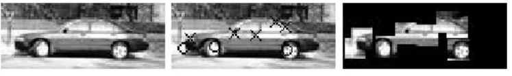
Fig. 1. Left: A sample object image used in vocabulary construction.
Center: Interest points detected by the F¨orstner operator. Crosses denote intersection points; circles denote centers of circular patterns.
Right: Patches extracted around the interest points.
A. Vocabulary Construction
The first stage in the approach is to develop a vocabulary of parts with which to represent images. To obtain an expressive representation for the object class of interest, we require distinctive parts that are specific to the object class but can also capture the variation across different instances of the object class. Our method for automatically selecting such parts is based on the extraction of interest points from a set of representative images of the target object. A similar method has been used in [21].
Interest points are points in an image that have high in-formation content in terms of the local change in signal. They have been used in a variety of problems in computer vision, including stereo matching [23], object recognition and image retrieval [24]. Interest points have typically been designed and used for properties such as rotation and view-point invariance, which are useful in recognizing different views of the same object, and not for the “perceptual” or “conceptual” quality that is required for reliably detecting different instances of an object class. However, by using interest points in conjunction with a redundant represen-tation that is described below, we are able to capture a certain degree of conceptual invariance.
We apply the F¨orstner interest operator [25], [21] to a set of representative images of the object class; this detects intersection points of lines and centers of circular patterns. Small image patches are then extracted around the inter-est points obtained. The goal of extracting a large set of patches from different instances of the object class is to be able to “cover” new object instances, i.e. to be able to represent new instances using a subset of these patches.
In our experiments, the F¨orstner operator was applied to a set of 50 representative images of cars, each 100×40 pixels in size. Figure 1 shows an example of this process. Patches of size 13×13 pixels were extracted around each such interest point, producing a total of 400 patches from the 50 images. These patches are shown in Figure 2.
As seen in Figure 2, several of the patches extracted by
Fig. 3. Examples of some of the “part” clusters formed after grouping similar patches together. These form our part vocabulary.
this procedure are visually very similar to each other. To facilitate learning, it is important to abstract over these patches by mapping similar patches to the same feature id (and distinct patches to different feature ids). This is achieved via a bottom-up clustering procedure. Initially, each patch is assigned to a separate cluster. Similar clus-ters are then successively merged together until no similar clusters remain. In merging clusters, the similarity between two clustersC1andC2is measured by the average similar-ity between their respective patches:
similarity(C1, C2) = 1
|C1||C2|
X
p1∈C1
X
p2∈C2
similarity(p1, p2),
where the similarity between two patches is measured by normalized correlation, allowing for small shifts of upto 2 pixels. Two clusters are merged if the similarity between them exceeds a certain threshold (0.80 in our implementa-tion). Using this technique, the 400 patches were grouped into 270 “part” clusters. While several clusters contained just one element, patches with high similarity were grouped together. Figure 3 shows some of the larger clusters that were formed. Each cluster as a whole is then given a single feature id and treated as a single “conceptual” part. In this way, by using a deliberately redundant representation that uses several similar patches to represent a single concep-tual part, we are able to extract a higher-level, concepconcep-tual representation from the interest points. The importance of the clustering procedure is demonstrated by experiments described in Section III-D.3.
B. Image Representation
Having constructed the part vocabulary above, images are now represented using this vocabulary. This is done by determining which of the vocabulary parts are present in an image, and then representing the image as a binary feature vector based on these detected parts and the spatial relations that are observed among them.
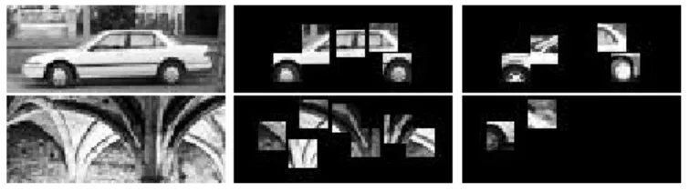
Fig. 4. Examples of the part detection process applied to a positive image (top row) and a negative image (bottom row) during training. Center images show the patches highlighted by the interest operator; notice how this successfully captures the interesting regions in the image. These highlighted interest patches are then matched with vocabulary parts. In the right images, the highlighted patches are replaced by an arbitrary member of the part cluster (if any) matched by this detection process. These parts, together with the spatial relations among them, form our representation of the image.
B.1 Part Detection
Since the vocabulary parts are all based on interest points, the search for parts in an image is restricted to interesting regions by first applying the same interest op-erator to the image and highlighting patches around the interest points found. For each such patch in the image, we perform a similarity-based indexing into the part vocab-ulary. The similarity of a vocabulary part P (which may be a cluster containing several patches) to a highlighted patchq is computed as
similarity(P, q) = 1
dλ|P|e
X
p∈P(λ,q)
similarity(p, q),
where 0 < λ ≤ 1, and P(λ,q) denotes the subset of the part cluster P that contains thedλ|P|epatches inP that are most similar to q. (In our implementation, λ = 0.5.) The similarity between patches p and q is measured by normalized correlation, allowing for small shifts of upto 2 pixels. For each highlighted patch q, the most similar vocabulary partP∗(q) is given by
P∗(q) = arg max
P similarity(P, q).
If a sufficiently similar vocabulary part is found, i.e. if similarity(P∗(q), q) exceeds a certain threshold (0.75 in our implementation), then the patch q in the image is repre-sented by the feature id corresponding to the vocabulary part P∗(q). Figure 4 shows examples of this process. B.2 Relations over Detected Parts
Spatial relations among the parts detected in an image are defined in terms of the distance and direction between each pair of parts. The distances and directions are dis-cretized into bins: in our implementation, the distances are defined relative to the part size and are discretized into 5 bins, while the directions are discretized into 8 differ-ent ranges, each covering an angle of 45◦. By considering the parts in a fixed order across the image, the number of direction bins that need to be represented is reduced to 4. This gives 20 possible relations (i.e. distance-direction combinations) between any two parts.
The 100×40 training images (and later, 100×40 windows in test images) that are converted to feature vectors have a very small number of parts actually present in them: on average, a positive window contains around 2-6 parts, while a negative one contains around 0-4. Therefore, the cost of computing relations between all pairs of detected parts is negligible once the parts have been detected.
B.3 Feature Vector
Each 100×40 training image (and later, each 100×
40 window in the test images) is represented as a feature vector containing feature elements of two types:
(i) Pn(i), denoting the ith occurrence of a part of type n
in the image (1 ≤ n ≤ 270 in our experiments; each n
corresponds to a particular part cluster),
(ii) R(mj)(Pn1, Pn2), denoting thejth occurrence of relation
Rmbetween a part of typen1and a part of typen2in the image (1≤m≤20 in our implementation; eachm corre-sponds to a particular distance-direction combination). These are binary features (each indicating whether or not a part or relation occurs in the image), each represented by a unique identifier1. The re-representation of the image is a list of the identifiers corresponding to the features that areactive (present) in the image.
C. Learning a Classifier
Using the above feature vector representation, a classi-fier is trained to classify a 100×40 image as car or non-car. We used a training set of 1000 labeled images (500 positive and 500 negative), each 100×40 pixels in size.2 The images were acquired partly by taking still photographs of parked cars, and partly by grabbing frames from digitized video sequences of cars in motion. The photographs and video sequences were all taken in the Champaign-Urbana area. After cropping and scaling to the required size, histogram equalization was performed on all images to reduce sensi-tivity to changes in illumination conditions. The positive examples contain images of different kinds of cars against a variety of backgrounds, and include images of partially oc-cluded cars. The negative training examples include images of natural scenes, buildings and road views. Note that our training set is relatively small and all images in our data set are natural; we do not use any synthetic training images, as has been done, for example, in [8], [13], [18].
Each of these training images is converted into a feature vector as described in Section II-B. Note that the poten-tial number of features in any vector is very large, since there are 270 different types of parts that may be present, 20 possible relations between each possible pair of parts, and several of the parts and relations may potentially be repeated. However, in any single image, only a very small
1In the implementation, a part feature of the form P(i)
n is
rep-resented by a unique feature id which is an integer determined as a function of n and i. Similarly, a relation feature of the form
R(mj)(Pn1, Pn2) is assigned a unique feature id that is a function of m,n1,n2 andj.
2Note that the 50 car images used for constructing the part
number of these possible features is actually active. Taking advantage of this sparseness property, we train our classi-fier using the Sparse Network of Winnows (SNoW) learn-ing architecture [26], [27], which is especially well-suited for such sparse feature representations.3 SNoW learns a lin-ear function over the feature space using a variation of the feature-efficient Winnow learning algorithm [28]; it allows input vectors to specify only active features, and as is the case for Winnow, its sample complexity grows linearly with the number of relevant features and only logarithmically with the total number of potential features. A separate function is learned over the common feature space for each target class in the classification task. In our task, feature vectors obtained from object training images are taken as positive examples for the object class and negative exam-ples for the non-object class, and vice-versa. Given a new input vector, the learned function corresponding to each class outputs an activation value, which is the dot product of the input vector with the learned weight vector, passed through a sigmoid function to lie between 0 and 1. Classifi-cation then takes place via a winner-take-all decision based on these activations (i.e. the class with the highest activa-tion wins). The activaactiva-tion levels have also been shown to provide a robust measure of confidence; we use this prop-erty in the final stage as described in Section II-D below. Using this learning algorithm, the representation learned for an object class is a linear threshold function over the feature space, i.e. over the part and relation features. D. Detection Hypothesis Using the Learned Classifier
Having learned a classifier4 that can classify 100×40 images as positive or negative, cars can be detected in an image by moving a 100×40 window over the image and classifying each such window as positive or negative. How-ever, due to the invariance of the classifier to small trans-lations of an object, several windows in the vicinity of an object in the image will be classified as positive, giving rise to multiple detections corresponding to a single object in the scene. A question that arises is how the system should be evaluated in the presence of these multiple detections. In much previous work in object detection, multiple detec-tions output by the system are all considered to be correct detections (provided they satisfy the criterion for a correct detection; this is discussed later in Section III-B). How-ever, such a system fails both to locate the objects in the image, and to form a correct hypothesis about the number of object instances present in the image. Therefore in using a classifier to perform detection, it is necessary to have an-other processing step, above the level of the classification output, to produce a coherent detection hypothesis.
A few studies have attempted to develop such a pro-cessing step. A simple strategy is used in [14]: detected windows are partitioned into disjoint (non-overlapping)
3Software for SNoW is freely available fromhttp://L2R.cs.uiuc. edu/~cogcomp/.
4The SNoW parameters used to train the classifier were 1.25, 0.8,
4.0 and 1.0 respectively for the promotion and demotion rates, the threshold and the default weight.
groups, and each group gives a single detection, located at the centroid of the corresponding original detections. While this may be suitable for the face detection database used there, in general, imposing a zero-overlap constraint on detected windows may be too strong a condition. The system in [8] uses the very property of multiple detections to its advantage, taking the number of detections in a small neighborhood as a measure of the detector’s confidence in the presence of an object within the neighborhood; if a high confidence is obtained, the multiple detections are col-lapsed into a single detection located at the centroid of the original detections. Our approach also uses a confidence measure to correctly localize an object; however, this con-fidence is obtained directly from the classifier. In addition, our approach offers a more systematic method for dealing with overlaps; like [14], [8] also uses a zero-overlap strategy, which is too restrictive for general object classes.
As a more general solution to the problem, we develop the notion of aclassifier activation mapin the single-scale case, when objects are sought at a single, pre-specified scale, and aclassifier activation pyramidin the multi-scale case, when objects are sought at multiple scales. These can be generated from any classifier that can produce a real-valued activation or confidence value in addition to a binary classification output.
D.1 Classifier Activation Map for Single-Scale Detections In the single-scale case (where, in our case, cars are sought at a fixed size of 100×40 pixels), a fixed-size window (of size 100×40 pixels in our case) is moved over the image and the learned classifier is applied to each such window (represented as a feature vector) in the image. Windows classified as negative are mapped to a zero activation value; windows classified as positive are mapped to the activation value produced by the classifier. This produces a map with high activation values at points where the classifier has a high confidence in its positive classification. This map can then be analyzed to find high-activation peaks, giving the desired object locations.
We propose two algorithms for analyzing the classifier activation map obtained from a test image. The first al-gorithm, which we refer to as the neighborhood suppres-sion algorithm, is based on the idea of non-maximum sup-pression. All activations in the map start out as ‘unsup-pressed’. At each step, the algorithm finds the highest un-suppressed activation in the map. If this activation is the highest among all activations (both suppressed and unsup-pressed) within some pre-defined neighborhood, then the location of the corresponding window is output as a de-tection, and all activations within the neighborhood are marked as ‘suppressed’; this means they are no longer con-sidered as candidates for detection. If the highest unsup-pressed activation found is lower than some (supunsup-pressed) activation within the neighborhood, it is simply marked as suppressed. The process is repeated until all activations in the map are either zero or have been suppressed. The shape and size of the neighborhood used can be chosen ap-propriately depending on the object class and window size.
In our experiments, we used a rectangular neighborhood of size 71 pixels (width)×81 pixels (height), centered at the location under consideration.
Our second algorithm for analyzing the classifier activa-tion map obtained from a test image is referred to as the repeated part elimination algorithm. This algorithm finds the highest activation in the map and outputs the loca-tion of the corresponding window as a detecloca-tion. It then removes all parts that are contained in this window, and re-computes the activation map by re-applying the classifier to the affected windows. This process is then repeated un-til all activations in the map become zero. This algorithm requires repeated application of the learned classifier, but avoids the need to determine appropriate neighborhood pa-rameters as in the neighborhood suppression algorithm.
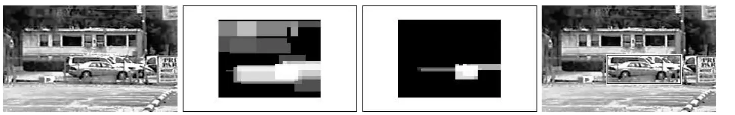
In both algorithms, there is a trade-off between the num-ber of correct detections and numnum-ber of false detections. An activation threshold is introduced in the algorithms to de-termine where to lie on this trade-off curve; all activations in the classifier activation map that fall below the thresh-old are automatically set to zero. Lowering the threshthresh-old increases the correct detections but also increases the false positives; raising the threshold has the opposite effect. Fig-ure 5 shows the classifier activation map generated from a sample test image, the map after applying a threshold, and the associated detection result (obtained using the neigh-borhood suppression algorithm).
D.2 Classifier Activation Pyramid for Multi-Scale Detec-tions
The approach described above for detecting objects at a single scale can be extended to detect objects at differ-ent scales in an image by processing the image at several scales. This can be done by scaling the input image a num-ber of times to form a multi-scale image pyramid, applying the learned classifier to fixed-size windows in each image in the pyramid, and forming a three-dimensional classifier activation pyramid instead of the earlier two-dimensional classifier activation map. This activation pyramid can then be analyzed to detect objects in both location and scale (analogous to finding peaks corresponding to object loca-tions in the two-dimensional map). In our multi-scale ex-periments, a test image is scaled to sizes ranging from 0.48 to 1.2 times the original size, each scale differing from the next by a factor of 1.2. The learned classifier is applied to 100×40 windows in each of the scaled images, resulting in a classifier activation pyramid with 6 scale levels.
Both the neighborhood suppression algorithm and the repeated part elimination algorithm used to analyze activa-tion maps in the single-scale case can be extended naturally to analyze activation pyramids in the multi-scale case. In this case, the algorithms output both the location and the scale of the window corresponding to an activation flagged as a detection. The neighborhood suppression algorithm now uses a three-dimensional neighborhood that extends across all scales; the neighborhood size at each scale is ob-tained by scaling the original neighborhood size with the image. Similarly, the repeated part elimination algorithm
now removes parts at all scales that arise from the region of an image contained within the window corresponding to an activation flagged as a detection. Again, an activa-tion threshold is introduced in the algorithms to determine where to lie in the trade-off between correct detections and false detections.
III. Evaluation
This section presents an experimental evaluation of the object detection approach developed in the previous sec-tion. The approach is evaluated both for the single-scale case and for the multi-scale case. We start by describing the data sets used for evaluation in Section III-A. In Sec-tions III-B and III-C we discuss in detail the evaluation criteria and performance measures we use. We emphasize the importance of identifying and specifying a suitable eval-uation methodology and discuss some important issues in this regard that have not been addressed satisfactorily in previous object detection research. Section III-D contains our experimental results.
A. Test Sets
We collected two sets of test images, the first for the single-scale case and the second for the multi-scale case. We refer to these as test set I and test set II, respectively. Test set I consists of 170 images containing 200 cars; the cars in this set are all roughly the same size as in the train-ing images. Test set II consists of 108 images containtrain-ing 139 cars; the cars in this set are of different sizes, ranging from roughly 0.8 to 2 times the size of cars in the train-ing images. The images were all taken in the Champaign-Urbana area, and were acquired in the same manner as the training images: partly from still images taken with a cam-era, and partly by grabbing frames from video sequences of cars in motion. They are of different resolutions and include instances of partially occluded cars, cars that have low contrast with the background, and images with highly textured backgrounds.
B. Evaluation Criteria
Past work on object detection has often emphasized the need for standardized data sets for comparing different ap-proaches. Although several studies have reported results on common data sets, it is often not clear how the different approaches have beenevaluated on these data sets. Prob-lems such as image classification have a naturally defined evaluation criterion associated with them. However, in ob-ject detection, there is no such natural criterion: correct detections and false detections can be defined in different ways, giving rising to different results. To ensure that the comparison between different approaches is truly fair, it is essential that the same evaluation criterion be used. There-fore in addition to standard data sets for object detection, we also need appropriate standardized evaluation criteria to be associated with them. Here we specify in detail the criteria we have used to evaluate our approach.5
5Both the data sets we have used and the evaluation routines are
Fig. 5. The second image shows the classifier activation map generated from the test image on the left; the activation at each point corresponds to the confidence of the classifier when applied to the 100×40 window centered at that point. The activations in the map have been scaled by 255 to produce the image; black corresponds to an activation of 0, white to an activation of 1. The third image shows the map after applying a threshold of 0.9: all activations below 0.9 have been set to zero. The activations in this map have been re-scaled; the activation range of 0.9-1 is now represented by the full black-white range. The bright white peak corresponds to the highest activation, producing the detection result shown on the right. The method prevents the system from producing multiple detections for a single object.
In the single-scale case, for each car in the test images, we determined manually the location of the best 100×40 window containing the car. For a location output by the detector to be evaluated as a correct detection, we require it to lie within an ellipse of a certain size centered at the true location. In other words, if (i∗, j∗) denotes the cen-ter of the window corresponding to the true location and (i, j) denotes the center of the window corresponding to the location output by the detector, then for (i, j) to be evaluated as a correct detection we require it to satisfy
|i−i∗|2
α2 height
+|j−j
∗|2
α2 width
≤1, (1)
where αheight, αwidth determine the size of the allowed el-lipse. We allowed the axes of the ellipse to be 25% of the object size along each dimension, thus taking αheight = 0.25×40 = 10 and αwidth= 0.25×100 = 25. In addition, if two or more locations output by the detector satisfy the above criterion for the same object, only one is considered a correct detection; the others are counted as false posi-tives (see Section II-D for a discussion on this). The above criterion is more strict than the criterion used in [29], and we have found that it corresponds more closely with human judgement.
In the multi-scale case, we determined manually both the location and the scale of the best window containing each car in the test images. Since we assume a fixed ratio between the height and width of any instance of the ob-ject class under study, the scale of the window containing an object can be represented simply by its width. The el-lipse criterion of the single-scale case is extended in this case to an ellipsoid criterion; if (i∗, j∗) denotes the center
of the window corresponding to the true location and w∗
its width, and (i, j) denotes the center of the window cor-responding to the location output by the detector and w
the width, then for (i, j, w) to be evaluated as a correct detection we require it to satisfy
|i−i∗|2
α2 height
+|j−j
∗|2
α2 width
+|w−w
∗|2
α2 scale
≤1, (2) where αheight, αwidth, αscale determine the size of the al-lowed ellipsoid. In this case, we alal-lowed the axes of the ellipsoid to be 25% of the true object size along each di-mension, thus takingαheight= 0.25×h∗,αwidth= 0.25×w∗
TABLE I
Symbols used in defining performance measurement quantities, together with their meanings.
TP Number of true positives
FP Number of false positives
nP Total number of positives in data set
nN Total number of negatives in data set
and αscale = 0.25×w∗, where h∗ is the height of the window corresponding to the true location (in our case,
h∗ = (40/100)w∗). Again, if two or more location-scale pairs output by the detector satisfy the above criterion for the same object, only one is considered a correct detection; the others are counted as false positives.
C. Performance Measures
In measuring the performance of an object detection ap-proach, the two quantities of interest are clearly the num-ber of correct detections, which we wish to maximize, and the number of false detections, which we wish to minimize. Most detection algorithms include a threshold parameter (such as the activation threshold in our case, described in Section II-D) which can be varied to lie at different points in the trade-off between correct and false detections. It is then of interest to measure how well an algorithm trades off the two quantities over a range of values of this parame-ter. Different methods for measuring peformance measure this trade-off in different ways, and again it is important to identify a suitable method that captures the trade-off correctly in the context of the object detection problem.
One method for expressing the trade-off is the receiver operating characteristics (ROC) curve. The ROC curve plots the true positive rate vs. the false positive rate, where
True positive rate = TP
nP, (3)
False positive rate = FP
nN, (4)
the symbols being explained in Table I. However, note that in the problem of object detection, the number of negatives in the data set, nN (required in the definition of the false positive rate in Eq. (4) above), is not defined. The num-ber of negative windows evaluated by a detection system
has commonly been used for this purpose. However, there are two problems with this approach. The first is that this measures the accuracy of the system as a classifier, not as a detector. Since the number of negative windows is typically very large compared to the number of posi-tive windows, a large absolute number of false detections appears to be small under this measure. The second and more fundamental problem is that the number of negative windows evaluated is not a property of either the input to the problem or the output, but rather a property internal to the implementation of the detection system.
When a detection system is put into practice, we are interested in knowing how many of the objects it detects, and how often the detections it makes are false. This trade-off is captured more accurately by a variation of the recall-precision curve, where
Recall = TP
nP, (5)
Precision = TP
TP+FP. (6) The first quantity of interest, namely the proportion of objects that are detected, is given by the recall (which is the same as the true positive rate in Eq. (3) above). The second quantity of interest, namely the number of false detections relative to the total number of detections made by the system, is given by
1−Precision = FP
TP+FP. (7) Plotting recall vs. (1−precision) therefore expresses the desired trade-off.
We shall also be interested in the setting of the threshold parameter that achieves the best trade-off between the two quantities. This will be measured by the point of highest F-measure, where
F-measure = 2·Recall·Precision
Recall + Precision . (8) The F-measure summarizes the trade-off between recall and precision, giving equal importance to both.
D. Experimental Results
We present our single-scale results in Section III-D.1 be-low, followed by a comparison of our approach with baseline methods in Section III-D.2 and a study of the contributions of different factors in the approach in Section III-D.3. Our multi-scale results are presented in Section III-D.4. D.1 Single-Scale Results
We applied our single-scale detector, with both the neighborhood suppression algorithm and the repeated part elimination algorithm (see Section II-D), to test set I (de-scribed in Section III-A), consisting of 170 images contain-ing 200 cars. To reduce computational costs, the 100×40 window was moved in steps of size 5% of the window size in each dimension, i.e. steps of 5 pixels and 2 pixels re-spectively in the horizontal and vertical directions in our
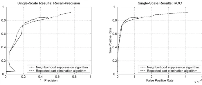
experiments. Training over 1000 images took around 10 minutes in our implementation on a machine with two Sun UltraSPARC-II 296 MHz processors and 1024 MB mem-ory. The time to test a 200×150 image was approximately 2.5 seconds.6 In all, 147,802 test windows were evaluated by the system, of which more than 134,333 were negative7. Following the discussion in Section III-C, we present our results as recall vs. (1−precision) in Figure 6. The different points on the curves are obtained by varying the activation threshold parameter as described in Section II-D. For com-parison, we also calculate the ROC curves as has been done before (using the number of negative windows evaluated by the system as the total number of negatives); these are also shown in Figure 6.
Tables II–III show some sample points from the recall-precision curves of Figure 6.8 Again, for comparison, we also show the false positive rate at each point correspond-ing to the ROC curves. The repeated part elimination algorithm allows for a higher recall than the neighborhood suppression algorithm. However, the highest F-measure achieved by the two algorithms is essentially the same.
Figures 7–8 show the output of our detector on some sample test images.
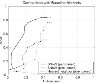
D.2 Comparison with Baseline Methods
As baselines for comparison, we implemented two addi-tional detection systems. The first is a SNoW-based de-tector that simply uses single pixel intensities (discretized into 16 intensity ranges) as features. Since this uses the same learning algorithm as our system and differs only in the representation, it provides a good basis for judging the importance of representation in learning. The second baseline system is a nearest-neighbor based detector that uses the normalized correlation between test windows and training images (in raw pixel intensity representation) as the similarity measure. The classifier activation map for the SNoW-based method was computed as before, using SNoW activations. In the case of nearest-neighbor, the classifier activation for a positively classified test window was taken to be the correlation of the window with the nearest training image. The results (using the neighbor-hood suppression algorithm) are shown in Figure 9. The poor performance of the baseline detectors is an indicator of the difficulty level of our test set: for the COIL object database, nearest-neighbor gives above 95% recognition ac-curacy, while on the face detection database in [13], the pixel-based SNoW method achieves above 94% recall.
6The improvements in computation time over [29] are mainly due
to two factors: a faster method for computing correlations, and the observation that image patches in test images need not be compared to vocabulary parts that are not seen during training.
7The number of negative windows was calculated by counting the
windows outside the permissible ellipses around objects (see Sec-tion III-B). However, since only one window within the permissible ellipse for any object would be counted as positive in evaluation, the effective number of negatives is actually larger than this number.
8The reason for the lower numbers in Table II compared to [29] is
Fig. 6. Left:Recall-precision curves showing the performance of our single-scale car detection system with the two algorithms described in Section II-D. Right:ROC curves showing the same results. It is important to note that the x-axis scales in the two curves are different; the x-axis values in the ROC curve are much smaller than in the recall-precision curve. Note also that precision need not necessarily decrease monotonically with increasing recall; this is exhibited by the inward bend on the lower left corner of the first curve (consequently, recall is not necessarily a function of precision). See Section III-C for definitions of the different quantities and a discussion of why the recall-precision curve is a more appropriate method for expressing object detection results than the ROC curve.
TABLE II
Performance of our single-scale detection system with the neighborhood suppression algorithm (see Section II-D) on test set I, containing 200 cars. Points of highest recall, highest precision and highest F-measure are shown in bold.
Activation No. of correct No. of false Recall,R Precision,P F-measure False positive threshold detections,TP detections,FP TP/200 TP/(TP+FP) 2·R·P/(R+P) rate,FP/134333
0.40 169 140 84.5 % 54.69 % 66.40 % 0.104 %
0.55 168 107 84.0 % 61.09 % 70.74 % 0.080 % 0.65 166 89 83.0 % 65.10 % 72.97 % 0.066 % 0.75 161 67 80.5 % 70.61 % 75.23 % 0.050 % 0.85 153 44 76.5 % 77.66 % 77.08 % 0.033 % 0.90 141 32 70.5 % 81.50 % 75.60 % 0.024 % 0.95 120 26 60.0 % 82.19 % 69.36 % 0.019 % 0.99 79 6 39.5 % 92.94 % 55.44 % 0.004 % 0.999 35 1 17.5 % 97.22 % 29.66 % 0.001 % 0.99995 8 0 4.0 % 100.0 % 7.69 % 0.0 %
TABLE III
Performance of our single-scale detection system with the repeated part elimination algorithm (see Section II-D) on test set I, containing 200 cars. Points of highest recall, highest precision and highest F-measure are shown in bold.
Activation No. of correct No. of false Recall,R Precision,P F-measure False positive threshold detections,TP detections,FP TP/200 TP/(TP+FP) 2·R·P/(R+P) rate,FP/134333
0.20 183 557 91.5 % 24.73 % 38.94 % 0.415 %
0.40 177 302 88.5 % 36.95 % 52.14 % 0.225 % 0.55 166 165 83.0 % 50.15 % 62.52 % 0.123 % 0.65 162 117 81.0 % 58.06 % 67.64 % 0.087 % 0.75 156 70 78.0 % 69.03 % 73.24 % 0.052 % 0.85 145 33 72.5 % 81.46 % 76.72 % 0.025 % 0.90 132 23 66.0 % 85.16 % 74.37 % 0.017 % 0.95 114 15 57.0 % 88.37 % 69.30 % 0.011 % 0.99 78 5 39.0 % 93.98 % 55.12 % 0.004 % 0.999 35 1 17.5 % 97.22 % 29.66 % 0.001 % 0.99995 8 0 4.0 % 100.0 % 7.69 % 0.0 %
D.3 Contributions of Different Factors
To gain a better understanding of the different factors contributing to the success of our approach, we conducted experiments in which we eliminated certain steps of our
method. The results (using the neighborhood suppression algorithm) are shown in Figure 10. In the first experiment, we eliminated the relation features, representing the im-ages simply by the parts present in them. This showed a
Fig. 7. Examples of test images on which our single-scale detection system achieved perfect detection results. Results shown are with the neighborhood suppression algorithm (see Section II-D) at the point of highest F-measure from Table II, i.e. using an activation threshold of 0.85. The windows are drawn by a separate evaluator program at theexactlocations output by the detector.
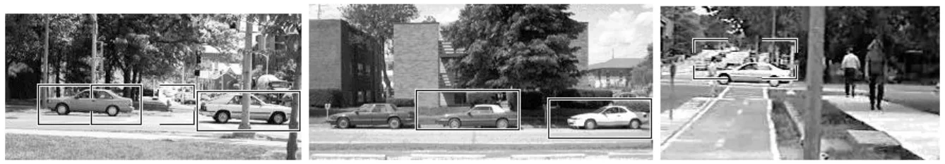
Fig. 8. Examples of test images on which our single-scale detection system missed objects or produced false detections. As in Figure 7, results shown are with the neighborhood suppression algorithm using an activation threshold of 0.85. The evaluator program draws a window ateachlocation output by the detector; locations evaluated as false positives are displayed with broken windows.
decrease in performance, suggesting that some additional information is captured by the relations. In the second ex-periment, we retained the relation features, but eliminated the patch clustering step when constructing the part vo-cabulary, assigning a different feature id to each of the 400 patches extracted from the sample object images. This re-sulted in a significant decrease in performance, confirming our intuition that representing similar patches as a sin-gle conceptulevel part is important for the learning al-gorithm to generalize well. We also tested the intuition that a small number of conceptual parts corresponding to frequently-seen patches should be sufficient for successful detection by ignoring all one-patch clusters in the part vo-cabulary. However, this decreased the performance, sug-gesting that the small clusters also play an important role. To further investigate the role of the patch clustering process, we studied the effect of the degree of clustering by varying the similarity threshold that two clusters are required to exceed in order to be merged into a single clus-ter (as mentioned in Section II-A, the threshold we have used is 0.80). The results of these experiments (again with the neighborhood suppression algorithm) are shown in Fig-ure 11. The results indicate that the threshold we have used (selected on the basis of visual appearance of the clusters formed) is in fact optimal for the learning algorithm.
Low-ering the threshold leads to dissimilar patches being as-signed to the same cluster and receiving the same feature id; on the other hand, raising the threshold causes patches that actually represent the same object part, but do not cross the high cluster threshold, to be assigned to different clusters and be treated as different parts (features). Both lead to poorer generalization.
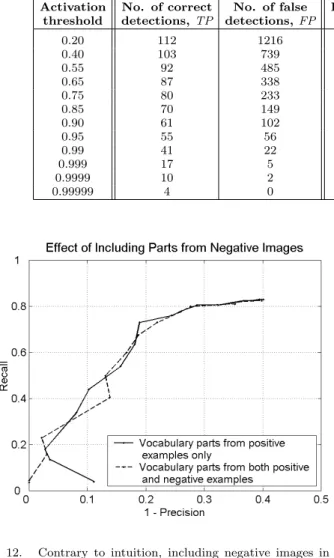
Another experiment we conducted was to include parts derived from negative (non-object) images in the part vocabulary; the intuition was that this should facilitate more accurate representation of negative images and should therefore improve detection results. To test this intuition, we removed 50 negative images from the training set and added them to the set of 50 object images that were orig-inally used in vocabulary construction. Using all 100 of these images to construct the part vocabulary, we then trained the classifier on 450 positive and 450 negative im-ages. The results, shown in Figure 129, suggest that con-structing the part vocabulary from only positive exam-ples of an object class gives an adequate representation
9Note that, in order to make a fair comparison, the top (solid) curve
in Figure 12 was obtained using only the same 450 positive and 450 negative images for training as the lower (dashed) curve. For this reason, it is different from the curve shown in previous figures (which uses 500 positive and 500 negative training images).
Fig. 11. Effect of degree of clustering. Left:Lowering the clustering threshold causes dissimilar patches to be clustered together, leading to poor generalization. Right:Raising the threshold causes patches representing the same object part to be assigned to different clusters; this again leads to poor generalization.
Fig. 9. Comparison of our detection system with baseline methods. The poor performance of the baseline methods is an indicator of the difficulty level of our test set. In addition, the poor performance of the pixel-based detector that uses the same learning algorithm as ours, and differs only in the representation, demonstrates the importance of choosing a good representation.
for learning to detect instances of the object class. D.4 Multi-Scale Results
Finally, we applied our multi-scale detector, with both the neighborhood suppression algorithm and the repeated part elimination algorithm, to test set II (described in Sec-tion III-A), consisting of 108 images containing 139 cars. As described in Section II-D.2, images were scaled to sizes ranging from 0.48 to 1.2 times the original size, each scale differing from the next by a factor of 1.2; a 100×40 window was then moved over each scaled image. As in the single-scale case, the window was moved in steps of 5 pixels in the horizontal direction and 2 pixels in the vertical direction.
Fig. 10. Contributions of different factors in our approach to the over-all performance. Both the relation features and the patch clustering step are important elements in our representation. Small clusters also have a role to play.
The time to test a 200×150 image was approximately 12 seconds. In all, 989,106 test windows were evaluated by the system, of which over 971,763 were negative10.
Our multi-scale results are shown in Figure 13 and Ta-bles IV–V. There are two observations to be made about these results. First, as in the single-scale case, the repeated part elimination algorithm allows for a higher recall than the neighborhood suppression algorithm (in this case, much higher, albeit at a considerable loss in precision). In terms of the highest F-measure achieved, however, the perfor-mance of the two algorithms is again similar.
The second observation about the multi-scale results is
10The number of negative windows was calculated as in the
TABLE IV
Performance of our multi-scale detection system with the neighborhood suppression algorithm (see Section II-D) on test set II, containing 139 cars. Points of highest recall, highest precision and highest F-measure are shown in bold.
Activation No. of correct No. of false Recall,R Precision,P F-measure False positive threshold detections,TP detections,FP TP/139 TP/(TP+FP) 2·R·P/(R+P) rate,FP/971763
0.65 70 215 50.36 % 24.56 % 33.02 % 0.0221 %
0.75 69 180 49.64 % 27.71 % 35.57 % 0.0185 % 0.85 65 126 46.76 % 34.03 % 39.39 % 0.0130 % 0.90 60 100 43.17 % 37.50 % 40.13 % 0.0103 % 0.95 54 56 38.85 % 49.09 % 43.37 % 0.0058 % 0.99 43 24 30.94 % 64.18 % 41.75 % 0.0025 % 0.999 18 7 12.95 % 72.0 % 21.95 % 0.0007 % 0.9999 10 2 7.19 % 83.33 % 13.25 % 0.0002 % 0.99999 4 0 2.88 % 100.0 % 5.59 % 0.0 %
TABLE V
Performance of our multi-scale detection system with the repeated part elimination algorithm (see Section II-D) on test set II, containing 139 cars. Points of highest recall, highest precision and highest F-measure are shown in bold.
Activation No. of correct No. of false Recall,R Precision,P F-measure False positive threshold detections,TP detections,FP TP/139 TP/(TP+FP) 2·R·P/(R+P) rate,FP/971763
0.20 112 1216 80.58 % 8.43 % 15.27 % 0.1251 %
0.40 103 739 74.10 % 12.23 % 21.00 % 0.0760 % 0.55 92 485 66.19 % 15.94 % 25.70 % 0.0499 % 0.65 87 338 62.59 % 20.47 % 30.85 % 0.0348 % 0.75 80 233 57.55 % 25.56 % 35.40 % 0.0240 % 0.85 70 149 50.36 % 31.96 % 39.11 % 0.0153 % 0.90 61 102 43.88 % 37.42 % 40.40 % 0.0105 % 0.95 55 56 39.57 % 49.55 % 44.0 % 0.0058 % 0.99 41 22 29.50 % 65.08 % 40.59 % 0.0023 % 0.999 17 5 12.23 % 77.27 % 21.12 % 0.0005 % 0.9999 10 2 7.19 % 83.33 % 13.25 % 0.0002 % 0.99999 4 0 2.88 % 100.0 % 5.59 % 0.0 %
Fig. 12. Contrary to intuition, including negative images in con-structing the part vocabulary does not seem to improve performance.
that they are considerably poorer than the single-scale re-sults; the highest F-measure drops from roughly 77% in the single-scale case to 44% in the multi-scale case. This certainly leaves much room for improvement in approaches for multi-scale detection. It is important to keep in mind, however, that our results are obtained using a rigorous
eval-Fig. 13. Performance of our multi-scale car detection system with the two algorithms described in Section II-D.
uation criterion (see Section III-B); indeed, this can be seen in Figures 14–15, which show the ouput of our multi-scale detector on some sample test images, together with the corresponding evaluations. In particular, our use of such a rigorous criterion makes previous results that have been reported for other approaches incomparable to ours.
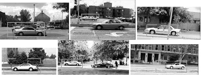
Fig. 14. Examples of test images on which our multi-scale detection system achieved perfect detection results. Results shown are with the neighborhood suppression algorithm (see Section II-D) at the point of highest F-measure from Table IV, i.e. using an activation threshold of 0.95. The windows are drawn by a separate evaluator program at theexactlocations and scales output by the detector.
Fig. 15. Examples of test images on which our multi-scale detection system missed objects or produced false detections. As in Figure 14, results shown are with the neighborhood suppression algorithm using an activation threshold of 0.95. The evaluator program draws a window ateachlocation-scale pair output by the detector; location-scale pairs evaluated as false positives are displayed with broken windows. Notice the rigorousness of the evaluation procedure (for details see Section III-B).
IV. Analysis
In this section we analyze the performance of individ-ual steps in our approach. In particular, we consider the results of applying the F¨orstner interest operator, of match-ing the image patches around interest points with vocabu-lary parts, and of applying the learned classifier.
A. Performance of Interest Operator
The first step in applying our detection approach is to find interest points in an image. Table VI shows the num-ber of interest points found by the F¨orstner interest op-erator in positive and negative image windows.11 In Fig-ure 16 we show histograms over the number of interest
11As before, in test images, all windows falling within the
permis-sible ellipses/ellipsoids around objects were counted as positive; all others were counted as negative.
points found. Positive windows mostly have a large num-ber of interest points; over 90% positive windows in train-ing, and over 75% in test set I and 70% in test set II, have 5 or more interest points. Negative windows have a more uniform distribution over the number of interest points in the training images, but mostly have a small number of interest points in test images; over 60% in test set I and over 75% in test set II have less than 5 interest points. B. Performance of Part Matching Process
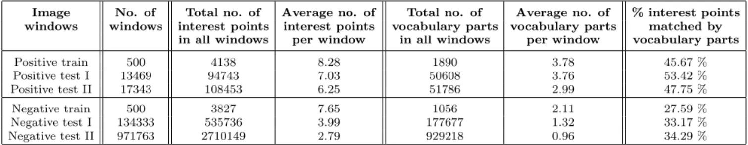
Once interest points have been found and image patches around them highlighted, the next step is to find vocabu-lary parts that match the highlighted patches. The result of this step is important since it determines the actual repre-sentation of an image window that is given to the classifier. Table VI shows the number of vocabulary parts found in positive and negative image windows. The proportion of
TABLE VI
Numbers of interest points and vocabulary parts found in positive and negative image windows.
Image No. of Total no. of Average no. of Total no. of Average no. of % interest points windows windows interest points interest points vocabulary parts vocabulary parts matched by
in all windows per window in all windows per window vocabulary parts
Positive train 500 4138 8.28 1890 3.78 45.67 % Positive test I 13469 94743 7.03 50608 3.76 53.42 % Positive test II 17343 108453 6.25 51786 2.99 47.75 % Negative train 500 3827 7.65 1056 2.11 27.59 % Negative test I 134333 535736 3.99 177677 1.32 33.17 % Negative test II 971763 2710149 2.79 929218 0.96 34.29 %
Fig. 16. Histograms showing distributions over the number of interest points in positive and negative image windows.
Fig. 17. Histograms showing distributions over the number of vocabulary parts in positive and negative image windows.
highlighted patches matched by vocabulary parts is more or less the same across training images and both test sets; roughly 50% for positive windows and 30% for negative windows. Histograms over the number of vocabulary parts are shown in Figure 17; the distributions are similar in form to those over interest points. It is interesting to note that the distribution over the number of vocabulary parts
in positive windows in test set I is very close to that over the number of vocabulary parts in positive training images. C. Performance of Learned Classifier
The performance of the classifier is shown in Table VII. While its performance on test set I is similar to that on the training set, its performance on test set II is drastically
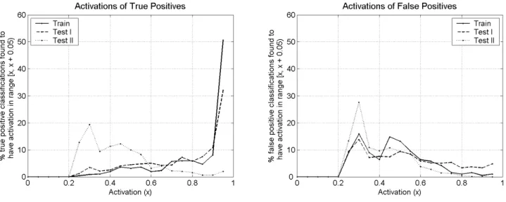
Fig. 18. Histograms showing distributions over the activation value produced by the learned classifier in the case of true positive classifications (positive windows correctly classified as positive) and false positive classifications (negative windows incorrectly classified as positive).
TABLE VII
Performance of raw classifier on positive and negative image windows.
Image No. of No. of correct Classification windows windows classifications accuracy
Positive train 500 470 94.0 % Positive test I 13469 12054 89.49 % Positive test II 17343 4935 28.46 % Negative train 500 311 62.2 % Negative test I 134333 75885 56.49 % Negative test II 971763 797432 82.06 %
different. In particular, the classification accuracy on pos-itive windows in test set II is very low. Furthermore, as is seen from Figure 18, positive windows in test set II that are classified correctly are done so with lower confidence than in test set I and the training set; the activations for true and false positives are well-separated in test set I and the training set, but the opposite is true for test set II. These observations shed some light on our multi-scale results, al-though it remains to be understood why the performance of the classifier differs in the two cases.
V. Conclusion
To summarize, we have presented an approach for learn-ing to detect objects in images uslearn-ing a sparse, part-based representation. In our approach, a vocabulary of distinc-tive object parts is automatically constructed from a set of sample images of the object class of interest; images are then represented using parts from this vocabulary, to-gether with spatial relations observed among the parts. Based on this representation, a learning algorithm is used to automatically learn a classifier that distinguishes be-tween members and non-members of the object class. To detect instances of the object class in a new image, the learned classifier is applied to several windows in the im-age to generate what we term a classifier activation map
in the single-scale case and a classifier activation pyramid in the multi-scale case. The activation map or pyramid is then processed to produce a coherent detection hypothesis; we presented two algorithms for this process.
We also addressed several methodological issues that are important in evaluating object detection approaches. First, the distinction between classification and detection was highlighted, and a general method for producing a good detector from a classifier was developed. Second, we em-phasized the importance of specifying and standardizing evaluation criteria in object detection experiments; this is essential for comparisons between different approaches to be meaningful. As a step in this direction, we formulated rigorous, quantitative evaluation criteria for both single-scale and multi-single-scale cases. Finally, we argued that recall-precision curves are more appropriate than ROC curves for measuring the performance of object detection approaches. We presented a critical evaluation of our approach, for both the single-scale case and the multi-scale case, under the proposed evaluation standards. We evaluated it here on images containing side views of cars; the approach is easily extensible to other objects that have distinguishable parts in a relatively fixed spatial configuration.
There are several avenues for further research. The multi-scale detection problem is clearly harder than the single-scale one; much room seems to remain for improve-ment in this direction. One possibility is to incorporate scale information in the features; this may help improve the performance of the classifier. The general detection problem may also require detecting objects at different ori-entations; it may be possible to achieve this by learning a number of view-based classifiers as in [18], and extend-ing the classifier activation map or pyramid to incorporate activation information from the different views. Computa-tion time can be reduced by processing different scales and orientations in parallel.
de-tect several object classes at once. It also remains an open problem to formulate a learning problem that directly ad-dresses the problem of detection rather than classification.
Acknowledgements
We would like to thank Ashutosh Garg, David Kriegman, Cordelia Schmid and Dav Zimak for helpful discussions and comments. We are also grateful to the anonymous referees for several useful suggestions. This work was supported by NSF ITR grants IIS 00-85980 and IIS 00-85836.
References
[1] S. Ullman, High-level vision: object recognition and visual cog-nition, MIT Press, 1996.
[2] I. Biederman, “Recognition by components: A theory of human image understanding,” Psychological Review, vol. 94, pp. 115– 147, 1987.
[3] N. K. Logothetis and D. L. Sheinberg, “Visual object recog-nition,” Annual Review of Neuroscience, vol. 19, pp. 577–621, 1996.
[4] S. E. Palmer, “Hierarchical structure in perceptual representa-tion,” Cognitive Psychology, vol. 9, pp. 441–474, 1977. [5] E. Wachsmuth, M. W. Oram, and D. I. Perrett, “Recognition
of objects and their component parts: responses of single units in the temporal cortex of the macaque,” Cerebral Cortex, vol. 4, pp. 509–522, 1994.
[6] A. Mohan, C. Papageorgiou, and T. Poggio, “Example-based object detection in images by components,” IEEE Transactions on Pattern Analysis and Machine Intelligence, vol. 23, pp. 349– 361, 2001.
[7] A. J. Colmenarez and T. S. Huang, “Face detection with information-based maximum discrimination,” inProceedings of the IEEE Conference on Computer Vision and Pattern Recog-nition, 1997, pp. 782–787.
[8] H. A. Rowley, S. Baluja, and T. Kanade, “Neural network-based face detection,” IEEE Transactions on Pattern Analysis and Machine Intelligence, vol. 20, no. 1, pp. 23–38, 1998. [9] E. Osuna, R. Freund, and F. Girosi, “Training support vector
machines: an application to face detection,” in Proceedings of the IEEE Conference on Computer Vision and Pattern Recog-nition, 1997, pp. 130–136.
[10] M. Turk and A. Pentland, “Eigenfaces for recognition,”Journal of Cognitive Neuroscience, vol. 3, no. 1, pp. 71–86, 1991. [11] B. Moghaddam and A. Pentland, “Probabilistic visual learning
for object detection,” Proceedings of the Fifth International Conference on Computer Vision, 1995.
[12] Y. Amit and D. Geman, “A computational model for visual selection,” Neural Computation, vol. 11, no. 7, pp. 1691–1715, 1999.
[13] M-H. Yang, D. Roth, and N. Ahuja, “A SNoW-based face de-tector,” inAdvances in Neural Information Processing Systems 12, Sara A. Solla, Todd K. Leen, and Klaus-Rober M¨uller, Eds., 2000, pp. 855–861.
[14] P. Viola and M. Jones, “Rapid object detection using a boosted cascade of simple features,” inProceedings of the IEEE Confer-ence on Computer Vision and Pattern Recognition, 2001. [15] L. Shams and J. Spoeslstra, “Learning Gabor-based features
for face detection,” inProceedings of World Congress in Neural Networks, International Neural Network Society, 1996, pp. 15– 20.
[16] C. Papageorgiou and T. Poggio, “A trainable system for object detection,” International Journal of Computer Vision, vol. 38, no. 1, pp. 15–33, 2000.
[17] Y. LeCun, P. Haffner, L. Bottou, and Y. Bengio, “Object recognition with gradient-based learning,” inFeature Grouping, D. Forsyth, Ed., 1999.
[18] H. Schneiderman and T. Kanade, “A statistical method for 3D object detection applied to faces and cars,” inProceedings of the IEEE Conference on Computer Vision and Pattern Recognition, 2000, vol. 1, pp. 746–751.
[19] S. Ullman, E. Sali, and M. Vidal-Naquet, “A fragment-based approach to object representation and classification,” in Pro-ceedings of the Fourth International Workshop on Visual Form,
Carlo Arcelli, Luigi P. Cordella, and Gabriella Sanniti di Baja, Eds., 2001, pp. 85–100.
[20] S. Ullman, M. Vidal-Naquet, and E. Sali, “Visual features of intermediate complexity and their use in classification,”Nature Neuroscience, vol. 5, no. 7, pp. 682–687, 2002.
[21] M. Weber, M. Welling, and P. Perona, “Unsupervised learning of models for recognition,” inProceedings of the Sixth European Conference on Computer Vision, 2000, pp. 18–32.
[22] D. Roth, M-H. Yang, and N. Ahuja, “Learning to recognize three-dimensional objects,” Neural Computation, vol. 14, no. 5, pp. 1071–1103, 2002.
[23] H. P. Moravec, “Towards automatic visual obstacle avoidance,” inProceedings of the Fifth International Joint Conference on Artificial Intelligence, 1977.
[24] C. Schmid and R. Mohr, “Local greyvalue invariants for image retrieval,”IEEE Transactions on Pattern Analysis and Machine Intelligence, vol. 19, no. 5, pp. 530–535, 1997.
[25] R. M. Haralick and L. G. Shapiro,Computer and Robot Vision II, Addison-Wesley, 1993.
[26] A. J. Carlson, C. Cumby, J. Rosen, and D. Roth, “The SNoW learning architecture,” Tech. Rep. UIUCDCS-R-99-2101, UIUC Computer Science Department, May 1999.
[27] D. Roth, “Learning to resolve natural language ambiguities: A unified approach,” in Proceedings of the Fifteenth National Conference on Artificial Intelligence, 1998, pp. 806–813. [28] Nick Littlestone, “Learning quickly when irrelevant attributes
abound: A new linear-threshold algorithm,”Machine Learning, vol. 2, no. 4, pp. 285–318, 1988.
[29] S. Agarwal and D. Roth, “Learning a sparse representation for object detection,” inProceedings of the Seventh European Con-ference on Computer Vision, 2002, vol. 4, pp. 113–130.