The Relationship Between Crude Oil and Natural Gas Prices

(1)

The Relationship Between Crude Oil and Natural Gas Prices

by

Jose A. Villar Natural Gas Division

Energy Information Administration and

Frederick L. Joutz Department of Economics The George Washington University

Abstract: This paper examines the time series econometric relationship between the Henry Hub natural gas price and the West Texas Intermediate (WTI) crude oil price. Typically, this relationship has been approached using simple correlations and deterministic trends. When data have unit roots as in this case, such analysis is faulty and subject to spurious results. We find a cointegrating relationship relating Henry Hub prices to the WTI and trend capturing the relative demand and supply effects over the 1989-through-2005 period. The dynamics of the relationship suggest a 1-month temporary shock to the WTI of 20 percent has a 5-percent contemporaneous impact on natural gas prices, but is dissipated to 2 percent in 2 months. A permanent shock of 20 percent in the WTI leads to a 16 percent increase in the Henry Hub price 1 year out all else equal.

Acknowledgements: The authors have benefited from comments and suggestions by William Trapmann, Nancy Kirkendall, Glenn Sweetnam, John Conti, Andy Kydes, and attendees of the Meeting of the American Statistical Association Committee on Energy Statistics with the EIA on April 7, 2006, particularly William Helkie, Cutler Cleveland, and Howard Gruenspecht.

(2)

2

Introduction

Economic theory suggests that natural gas and crude oil prices should be related because natural gas and crude oil are substitutes in consumption and also complements, as well as rivals, in production. In general, the observed pattern of crude oil and natural gas prices tend to support this theory (Figure 1). However, there have been periods in which natural gas and crude oil prices have appeared to move independently of each other. Furthermore, over the past 5 years, periods when natural gas prices have appeared to decouple from crude oil prices have been occurring with increasing frequency with natural gas prices rising above its historical relationship with crude oil prices in 2001, 2003, and again in 2005. This has led some to examine whether natural gas and crude oil prices are related (For example, see Brown (2005), Panagioditis and Rutledge (2004), and Jabir (2006)).

Economic factors link oil and natural gas prices through both supply and demand. Market behavior suggests that past changes in the oil price drove changes in the natural gas price, but the converse did not appear to occur. One reason for the asymmetric relationship is the relative size of each market. The crude oil price is determined on the world market, while natural gas markets, at least for the period of investigation, tend to be regionally segmented. Consequently, the domestic natural gas market is much smaller than the global crude oil market, and events or conditions in the U.S. natural gas market seem unlikely to be able to influence the global price of oil.

This paper seeks to develop an understanding of the salient characteristics of the economic and statistical relationship between oil and natural gas prices. The sample period covers January 1989 through December 2005 which includes:

• oil price spikes in 1990 following the invasion of Kuwait

• the oil price collapse from the supply glut in 1999

• dramatic oil price increases since 2003

• substantial natural gas regulatory reform

• significant supply shortages in cold winters

• the natural gas supply bubble for most of the 1990s

(3)

Figure 1: Henry Hub and West Texas Intermediate Prices (1989-2005)

2 4 6 8 10 12

20 30 40 50 60 70

1990 1995 2000 2005

P

ri

ce

(Do

ll

ars

p

er M

M

B

tu

) P_{rice (Do}

lla

rs

p

er B

arrel

)

HenryHub Natural Gas Price WTI Crude Oil Price

Source: Energy Information Administration, Short-Term Energy Outlook, various issues.

The analysis identifies the economic factors suggesting how crude oil and natural gas prices are related, and assesses the statistical significance of the relationship between the two over time. The focus of the econometric analysis is primarily on the movements in the prices; the economic factors are not explicitly modeled. Nevertheless, a significant stable relationship between the two price series is identified. Oil prices are found to influence the long-run development of natural gas prices, but are not influenced by them.

(4)

4

Economic Factors Linking Natural Gas and Crude Oil Prices Increases in oil prices may affect the natural gas market in several ways. Demand:

• An increase in crude oil prices motivates consumers to substitute natural gas for petroleum products in consumption, which increases natural gas demand and hence prices. Oil and natural gas are competitive substitutes primarily in the electric generation and industrial sectors of the economy. According to EIA’s 2002 Manufacturing Energy Consumption Survey (MECS), approximately 18 percent of natural gas usage can be switched to petroleum products. The National Petroleum Council (NPC) in its 2003 report estimated that approximately 5 percent of industrial boilers can switch between natural gas and petroleum fuels (Costello, Huntington, and Wilson, (2005)). Other analysts estimate that up to 20 percent of power generation capacity is dual-fired, although in practice it is assumed that the relevant percentage is considerably less. However, fuel-switching is not limited to dual-fired units. Some degree of additional fuel switching is achieved by dispatching decisions to switch from single-fired boilers of one type to that of another fuel. Although these are limited percentages, the shift in marginal consumption can have a pronounced impact on prices in a tight market.

Supply:

• Increases in crude oil prices resulting from an increase in crude oil demand may increase natural gas produced as a co-product of oil, which would tend to decrease natural gas prices. Natural gas is found in two basic forms—associated gas and non-associated gas. Associated natural gas is natural gas that occurs in crude oil reservoirs either as free gas (associated) or as gas in solution with crude oil (dissolved gas). Non-associated gas is natural gas that is not in contact with significant quantities of crude oil in the reservoir. In 2004, associated-dissolved gas comprised approximately 2.7 trillion cubic feet (Tcf) or 14 percent of marketed natural gas production in the United States.

• An increase in crude oil prices resulting from an increase in crude oil demand may lead to increased costs of natural gas production and development, putting upward pressure on natural gas prices. Natural gas and crude oil operators compete for similar economic resources such as labor and drilling rigs. An increase in the price of oil would lead to

(5)

higher levels of drilling or production activities as operators explored for and developed oil prospects at a higher rate. The increased activity would bid up the cost of the relevant factors, which will increase the cost of finding and developing natural gas prospects.

• An increase in crude oil prices resulting from an increase in crude oil demand may lead to more drilling and development of natural gas projects, which would tend to increase production and decrease natural gas prices. Increased oil prices affect the cash flow available to finance new drilling and project development. Changes in the relative price structure could lead to increases in drilling for one fuel at the expense of the other. However, it is generally expected that increased cash flow would expand supply activities for both natural gas and oil.

Finally, another factor linking the natural gas and crude oil markets is liquefied natural gas (LNG), which permits the transoceanic delivery of natural gas from remote gas-producing countries to large gas-consuming areas such as the Lower 48 States. LNG imports to the Lower 48 States may affect the relative economics of crude oil and natural gas to the extent that natural gas consumption occurs at the margin. Most LNG contracts are indexed on oil prices, directly linking natural gas and crude oil prices (Foss, 2005). While most of these indexed contracts occur primarily in the Pacific Basin, short-term markets for LNG are developing on either side of the Atlantic Basin in the United States and Spain, facilitating interregional gas price competition between the United States and Europe (Jensen, 2003). A “world market” for natural gas likely would reinforce the linkages between natural gas and crude oil prices.

These economic factors suggest that oil and natural gas prices should be related. The analysis of crude oil and natural gas prices that follows empirically tests this hypothesis by drawing on the extensive time series literature on nonstationary processes and cointegration.1 In general, it should not be possible to form a weighted average of two nonstationary variables and create a stationary time series. However, in certain cases when two variables share common stochastic or deterministic trends, it is possible to create such a cointegrating relationship. Because cointegrated variables share an intrinsic structural relationship over time, empirically testing for

(6)

6

the presence of cointegration constitutes an empirical test of the long-run relationship between the variables.

The analysis is presented in five sections and proceeds as follows.

• The key time series concepts used in the analysis are presented, focusing on the properties of nonstationary variables and how they relate to the notion of cointegration.

• The time series properties of natural gas and crude oil prices are examined.

• A vector autoregression (VAR) model is estimated to capture the dynamic properties of the time series and test for cointegration. The existence of cointegration is used to identify a possible long-run relationship and examine its feedback into the two price series.

• The cointegrating relation estimated in the earlier preceding stage of the analysis is used to determine an error correction mechanism for modeling natural gas prices in a conditional error correction model.

• The implications and price dynamics of this model are explored. The paper concludes with a summary of the findings and directions for further research and potential applications to EIA modeling and forecasting issues.

The analysis in this paper provides statistical evidence supporting the hypothesis that natural gas and crude oil prices are nonstationary time series. Modeling energy data without taking into account possible nonstationarity in the data could lead researchers to miss important features and properties of the data, which could lead to spurious or misleading results in estimation, forecasting, and policy analysis. Cointegration analysis provides an effective method to resolve the issues associated with nonstationary data without the loss of information associated with other forms of restoring stationarity to nonstationary data. Key highlights of the cointegration analysis of natural gas and crude oil prices include:

• A stable statistically significant relationship between the Henry Hub natural gas price and the WTI crude oil price and trend capturing the relative demand and supply effects over the 1989-through-2005 period was identified.

• Natural gas and crude oil prices have had a stable long-run relationship despite periods when a large exogenous spike in either crude oil or natural gas prices may have produced

(7)

the appearance that these two prices had decoupled.

• There is a statistically significant trend term, suggesting that natural gas prices appear to be growing at a slightly faster rate than crude oil prices, narrowing the gap between the two over time.

Key Time Series Concepts

Characteristics of Stationary and Nonstationary Time Series

Econometric analysis of the classical linear regression model depends heavily on the assumption that observed data result from stationary data generation processes. However, in practice many economic time series are nonstationary (Nelson and Plosser, 1982). Stationary time series evolve independently of time. Specifically, stationarity requires that random shocks or innovations tend to dissipate and not have any lasting effects on the evolution of the time series.2 Similarly, the variance is assumed to be constant – independent of time. In contrast, nonstationary time series have permanent effects resulting from random shocks. For example, consider the following autoregressive process:

1

t t t

y = ρy₋ + u (1)

where ut is assumed to be a purely random variable that is normally, independently, and

identically distributed with mean zero and variance σ2.

Given a value of ρ in equation (1) above, yt can be solved recursively as a function of an initial y, time, and the sum of the random disturbances.

0 1

t

t t i

t i

i

y ρ y ρ −u

=

= +

∑

(2)

The expression in equation (2) may be either stationary or nonstationary. If |ρ| is less than 1, random shocks to the system dissipate with time, and yt is a stationary process. This occurs because ρiapproaches zero asymptotically as i increases. Because the impacts of random shocks

(8)

8

asymptotically converge to constants as t becomes larger. Consequently, stationary processes evolve independently of time. However, if ρ=1, it can be shown that:

0 1

t

t i

i

y y u

=

= +

∑

(3)

When ρ=1, yt is equal to the sum of all past shocks and an initial starting condition, y0, such that all past disturbances have a permanent effect on yt. In other words, a random shock that is far-removed from the current period will have as much an impact on the current period as a random shock of equal magnitude in the current period. As a result, it can be shown that the variance and autocovariance increase with time, depending on the initial starting conditions. It is the time-varying nature of the variance and autocovariance that generally cause the failure of the assumptions underlying the classical linear regression model: no autocorrelation, homoskedasticity, and multivariate normality. A fundamental challenge in the analysis of energy and economic time series is the nonstationarity of many economic variables. For example, one well-known issue associated with nonstationary variables is the problem of spurious regressions, in which a regression of two unrelated nonstationary variables—each trending upward over time—may result in a high R2_{suggesting a tight fit of the data when the model in fact explains}

nothing but the similar rising trend over time.

Stochastic processes such as in equation (3) are called unit roots, because ρ=1. A nonstationary time series such as in equation (3) is fundamentally evolutionary in nature. Starting from the initial point, y0, yt will either increase or decrease depending on the random outcome of ut in a given period, accumulating each of the random shocks in each period. Consequently nonstationary time series tend to exhibit “wandering” behavior as they follow a stochastic trend—a trend with random increments. This contrasts with a deterministic trend that has constant increments.

At any given point in time, a particular observation of a nonstationary time series with a unit root essentially results from a summation of all the past random errors that preceded it. This process is called integration because the present outcome incorporates all of the random errors in the past. A simple way of solving the problem of integration in a given time series is simply to subtract the value of the preceding period from the current period, which has the effect of

(9)

canceling out the stochastic trends in the successive periods, and creating a stationary series. This transformation is called differencing. From equation (3), a stationary time series can be created from a nonstationary series such as yt, by focusing on the change between the periods.

1

t t t t

y y y₋ u

Δ = − = (4)

All integrated variables can be “de-trended” by differencing. However, some nonstationary variables must be differenced more than once—taking differences of differences—to create a stationary series. The order of integration refers to the number of times that the differencing operation must be performed to restore stationarity. For example, in equation (3) ytis integrated of order 1, or I(1).

While all I(k) variables can be differenced k times to generate a stationary time series, there are some I(1) variables that are cointegrated. This means that it is possible to form a stationary linear combination from two I(1) variables. In other words, given two variables xt and yt that are nonstationary I(1) variables: xt and yt are cointegrated if it is possible to form a linear combination such as:

0 '

t t t

y − β − β x = u (5)

where ut is a stationary I(0) variable.

Cointegration is similar to integration in that the process of detrending the nonstationary series involves focuses on the offsetting of the shared attributes of stochastic trends. In some economic applications it is advantageous to compare two or more time series for shared stochastic patterns over time. One advantage of cointegration is that it solves the problem of spurious regressions without having to difference the data and losing the information about the levels of the time series. Cointegration of economic time series suggests that the economic variables have a long-run structural relationship that can be empirically evaluated.

(10)

10

The Time Series Properties of the Henry Hub Natural Gas Price and the West Texas Intermediate (WTI) Crude Oil Price

A Simple Graphical and Statistical Analysis

Using 17 years of monthly data drawn from January 1989 through December 2005, time series of WTI crude oil and Henry Hub natural gas spot prices were analyzed, focusing on decomposing the short-run and long-run effects of changes in crude oil and natural gas prices. The time period of the analysis was determined by the availability of a complete series of both Henry Hub and WTI prices. Monthly series were used because they have sufficient texture to capture short-run movements over time, without adding unnecessary complexity to the analysis. The relationships at this frequency can have relevance for the Energy Information Administration’s (EIA) forecasting analysis used in the Short-Term Energy Outlook and Annual Energy Outlook.

The analysis of the time series properties of oil and natural gas prices begins by examining the levels and differences of natural gas and oil prices statistically and graphically. The two series are transformed to natural logarithms and presented in Figure 2. The logarithmic transformations were used to remove the scale effects in the variables and reduce the possible effect of heteroskedasticity. Logarithmic transformations also have the beneficial property of allowing estimated parameters to be directly interpreted as constant elasticities.3 Furthermore, logarithmic transformations allow the analysis to proceed on variables in the same units. To facilitate a more direct comparison of the two series in the graph, crude oil prices are mean-adjusted down to natural gas prices.4

While it is very difficult to tell if a time series is nonstationary by visual examination of level data, it appears that natural gas and crude oil prices do have characteristics consistent with nonstationary data. Both natural gas and crude oil prices have a trend and meandering quality, with prices wandering up and then down. The means of the series do not appear constant over time, and in fact may be drifting upward, suggesting the possibility of a stochastic trend. The price series also appear to be serially correlated, with prices drifting up for extended periods of successive months, followed by periods of successive declines. Furthermore, the volatility of the

3_{Throughout the remainder of the paper, the analysis will be conducted on logarithms of natural gas and crude} oil prices. For the sake of brevity, the terms price and logarithm of price will be used interchangeably unless otherwise noted.

4_{The transformation crude oil price series entails subtracting the mean of the logarithm of the Henry Hub price} from the logarithm of the WTI crude oil price.

(11)

series individually and jointly appears to vary over time. However, variation of the price series in Figure 2 seems consistent with the possibility that natural gas and crude oil share a common trend, fluctuating around a fixed level. These results suggest that natural gas and crude oil prices may be cointegrated.

Figure 2. Logarithm of Henry Hub Natural Gas Price and Mean-Adjusted Logarithm of West Texas Intermediate Crude Oil Prices (1989-2005)

1990 1995 2000 2005

0.25 0.50 0.75 1.00 1.25 1.50 1.75 2.00 2.25 2.50

P

ric

e (in

N

atu

ra

l L

og

arith

m

s)

HenryHub Natural Gas Price WTI Crude Oil Price

Source: Energy Information Administration, Natural Gas Division.

Figure 3 presents the two series in columns of their first differences and 12-month differences respectively. Both series appear stationary in their differences, although the departures from the mean appear more prolonged in the annual difference case. The analysis will only focus on the levels and first differences of the two series.

(12)

12

Figure 3. Henry Hub and West Texas Intermediate Prices:

First and 12-Month Differences in Natural Logarithms

1990 1995 2000 2005

-0.2 0.2

0.6 1-Month Difference (ln Henry Hub Price)

1990 1995 2000 2005

-0.2 0.0 0.2 0.4

1-Month Difference (ln WTI Price)

1990 1995 2000 2005

-1 0 1

P

ri

ce

C

ha

nge

(

in N

at

ur

al

L

oga

ri

th

ms)

12-Month Difference (ln Henry Hub Price)

1990 1995 2000 2005

-0.5 0.0 0.5

1.0 12-Month Difference (ln WTI Price)

The probability distributions and autocorrelation functions (ACFs) for the series are presented in Figures 4 and 5. Histograms summarize the frequency of occurrence that a variable falls within a certain range of values. As such, histograms provide insights into the mean, standard error, and probability distribution of a given variable. Histograms of WTI and Henry Hub prices are presented in the top panels of Figure 4, with a plot of a normal distribution superimposed over the histogram and a smooth line generated from the histogram. It is readily apparent that Henry Hub and WTI prices are not normally distributed. The probability distributions for both price series appear bimodal, skewed relative to the normal distribution. The ACFs through 12 lags of the WTI and Henry Hub prices are presented in the lower panel of the figure. The ACFs are highly significant, close to unity, and decay slowly with considerable persistence. These graphical and statistical findings are consistent with unit root processes, which have all

(13)

autocorrelations close to 1.

Figure 4. Henry Hub and West Texas Intermediate Prices Histogram and Autocorrelogram

Functions

-0.5 0.0 0.5 1.0 1.5 2.0 2.5 3.0

0.25 0.50 0.75 1.00 1.25

1.50 Henry Hub Natural Gas Prices

D

en

sity

Implied Empirical Distribution Normal Distribution (s.d.=0.543)

2.5 3.0 3.5 4.0 4.5

0.5 1.0 1.5 2.0

2.5 WTI Crude Oil Prices

0 5 10

0.25 0.50 0.75 1.00

A

uto

co

rr

el

atio

n

Autocorrelation Function (ln Henry Hub Price)

0 5 10

0.25 0.50 0.75 1.00

Autocorrelation Function (ln WTI Price)

Figure 5 contains histograms and ACFs for the first differences of both price series. In each case, the differencing transformation appears to have resolved the nonstationarities in the two series for the most part. In both cases, the probability distributions of the differenced series appear to be approximately normally distributed. Further, the autocorrelations are also much smaller, and statistically insignificant at most lags. These results support the concept that the levels of the price series are unit roots; they are integrated processes of order one, I(1). The problems associated with nonstationary data will be a key consideration in the model specification and estimation that follows.

(14)

14

Figure 5. First Differences of Henry Hub and West Texas Intermediate Prices Histogram and

Autocorrelogram Functions

-0.50 -0.25 0.00 0.25 0.50 1

2 3 4

5 First Difference Henry Hub Natural Gas Prices

De

ns

ity

-0.3 -0.2 -0.1 0.0 0.1 0.2 0.3 0.4 0.5 2

4 6

First Difference WTI Natural Gas Prices

0 5 10

-0.5 0.0 0.5 1.0 A ut oco rr el at io n

Autocorrelation Function (Dln Henry Hub Price)

0 5 10

-0.5 0.0 0.5 1.0

Autocorrelation Function (Dln WTI Price)

Testing for Unit Roots

The analysis proceeds with a more formal test of the integrated process. Two forms of the augmented Dickey-Fuller (ADF)5 test were estimated where each form differs in the assumed deterministic component(s) in the series:

0 1

;

P

t i t i t i t

i=1

P 2

t i t i t i t

i=1

y y + y

y y + * t y

constant only constant and trend

α α γ ε

α α α γ ε

− −

Δ = + Δ +

Δ = + + Δ +

∑

(6)

(15)

The εt is assumed to be a Gaussian white noise random error; and t=1,..., 204 (the number of observations in the sample) is a time trend term. The number of lagged differences, p, is chosen to ensure that the estimated errors are not serially correlated based on the Akaike Information Criterion (AIC) statistic.

Table 1 contains the results from the ADF tests. The top half of the table presents the test statistics that determine whether the series in levels are stationary I(0), and the bottom half of the table presents the findings on whether the first differences of the series are stationary I(1). There are seven columns in the table. The first column refers to the number of lags, p, in each regression. This is followed by two sets of three columns where the first set presents the results for the Henry Hub natural gas price tests and the second has the WTI crude oil price tests. The three columns for each set include the t-statistic for the ADF test that is associated with theα₁, the t-statistic on the last lagged difference variable in each equation, and the AIC. The null hypothesis in each test is that there is a unit root or the series is I(1); this implies that the coefficient α₁ is zero. Because of the properties of nonstationary series, the distributions of the statistics are different. The critical values are found at the bottom of the table. The t-DY lag and AIC measures are used in evaluating the appropriate number of lags in the testing procedure that remove serial correlation in the residuals.

The Henry Hub series appears to be an I(1) process. The t-ADF tests for the Henry Hub series appear to be significant at the 5-percent level of significance for lags 1 and 11, as the t-ADF values, -3.527 and -3.726, respectively, exceed the critical value of -3.43 in absolute value. This could lead to a rejection of the null hypothesis of a unit root; however further testing revealed these equation estimates were unstable due to the nonstationarity in the series including large outliers. The WTI series also appears to be an I(1) process, failing to reject the null hypothesis of a unit root at each of the 12 lags.

(16)

16

Table 1. Augmented Dickey-Fuller Tests for Unit Roots (Natural Gas Spot Price and West Texas

Intermediate Spot Crude Price)

lnHenryHub lnWTI Number of

Lags t-adf t-DY_lag AIC t-adf t-DY_lag AIC

12 -3.373 0.060 -4.003 -2.086 -0.040 -5.088

11 -3.527* 2.198 -4.013 -2.153 1.620 -5.099

10 -3.009 3.813 -3.996 -1.851 2.405 -5.095

9 -2.180 -0.322 -3.928 -1.418 0.055 -5.073

8 -2.312 -1.333 -3.938 -1.441 0.981 -5.083

7 -2.711 -1.302 -3.939 -1.276 -0.498 -5.089

6 -3.157 0.388 -3.940 -1.388 -0.423 -5.098

5 -3.180 0.938 -3.949 -1.504 0.089 -5.107

4 -3.041 1.334 -3.955 -1.519 -1.871 -5.118

3 -2.786 -1.120 -3.956 -1.953 -0.542 -5.109

2 -3.255 -0.838 -3.960 -2.130 -0.929 -5.118

1 -3.726* 2.836 -3.967 -2.397 3.834 -5.124

0 -3.080 -3.935 -1.729 -5.059

First Difference lnHenryHub First Difference lnWTI

Number of

Lags t-adf t-DY_lag AIC t-adf t-DY_lag AIC

12 -4.093** 1.808 -3.959 -3.608** 1.495 -5.078 11 -3.698** 0.925 -3.951 -3.332* 0.459 -5.076 10 -3.584** -1.286 -3.957 -3.331* -1.282 -5.085 9 -4.207** -3.266 -3.958 -3.840** -2.214 -5.087 8 -6.062** 0.708 -3.911 -4.850** 0.089 -5.070 7 -6.426** 1.844 -3.919 -5.177** -0.876 -5.081 6 -6.201** 2.000 -3.911 -6.076** 0.590 -5.087 5 -5.860** 0.435 -3.900 -6.473** 0.574 -5.096 4 -6.316** -0.140 -3.909 -6.994** 0.060 -5.104 3 -7.320** -0.632 -3.919 -8.131** 2.108 -5.115 2 -9.400** 1.905 -3.928 -8.137** 0.889 -5.102 1 -10.26** 1.862 -3.919 -9.223** 1.338 -5.108 0 -11.86** -3.911 -10.61** -5.109

Note: The sample period for the analysis is July 1989 through December 2005.

Note: Levels test has a constant and trend included. The critical values; 5 percent=-3.43 1 percent=-4.01. First differences test has a constant included. The critical values; 5 percent=-2.88 1 percent=-3.47.

(17)

VAR Model Specification, Estimation, and Testing for Cointegration

Specification of the VAR Model

A general to specific approach was employed in estimating the model as in Hendry (1986) and Hendry and Juselius (2000, 2001). First the lag structure of the VAR is determined. The VAR model is general enough to accommodate any number of lag structures, so this must be determined prior to conducting the analysis. Next, a simple unrestricted version of the VAR was estimated and evaluated for fit and stability. Based on these results, the model was refined and re-estimated. Once a correctly specified model emerges from this process, restrictions are imposed on the model, hypothesis testing is done, and the model results are interpreted.

The test for a long-run relationship between natural gas prices and crude oil prices starts with the estimation of the bivariate VAR system. The VAR can be specified in matrix notation as:

,1 1

,2 1

2 3

1 2 3

ln ln

( )

ln ln

( ) ...

t

t t

t

t t t

p p

HenryHub HenryHub constant

L B

WTI WTI timetrend

where L L L L L

ε ε −

−

⎡ ⎤

⎡ ⎤ ⎡ ⎤ ⎡ ⎤

= Π + _{+ ⎢ ⎥}

⎢ ⎥ ⎢ ⎥ ⎢ ⎥

⎣ ⎦ ⎣ ⎦ ⎣ ⎦ ⎣ ⎦

Π = Π + Π + Π + + Π

(7)

The price series have been transformed to natural logarithms to address heteroskedasticity issues. Constant and trend terms are included in each equation; their role will be modified at a later stage in the analysis. The two error terms are assumed to be white noise and can be contemporaneously correlated. The expression Π(L) is a lag polynomial operator indicating that p lags of each price is used in the VAR.6 The individual Πi terms represent a 2x2 matrix of

coefficients at the ith lag, and the B matrix is 2x2. The other variables, lnHenryHub, ln WTI, constant, timetrend, and the error terms, are scalar.

The number of lags to use in the model at the beginning is unknown. The selection methodology starts with an initial maximum of p lags which are assumed to be more than necessary. Residual diagnostic tests like normality, serial correlation, and heteroskedasticity are conducted, and the

(18)

18

assumption of white noise residuals. A large number of lags are likely to produce an over-parameterized model. However, any econometric analysis needs to start with a statistical model of the data generating process. Parsimony is achieved by testing for the fewest number of lags that can explain the dynamics in the data system.

Lag Length Selection

The selection criteria for the appropriate lag length of the unrestricted VAR models employ _χ2

test(s) and F-tests. Table 2 shows results for the former and Table 3 contains results for the latter. The maximum possible lag length considered was 6. The first three columns show the number of observations, number of lags, and estimated parameters for each VAR respectively. The log likelihood is given in the fourth column. The last three columns contain the Bayesian Schwartz Criterion (BSC), the Hannan-Quinn Criterion (HQ), and the Akaike Information Criterion (AIC), respectively.

Table 2. Tests of Lag Length or Model Reduction for VAR

T Lags parameters log-likelihood BSC HQ AIC

198 6 28 371.029 -3.000 -3.277 -3.465

198 5 24 368.076 -3.077 -3.314 -3.476

198 4 20 364.467 -3.147 -3.345 -3.480

198 3 16 363.027 -3.240 -3.398 -3.505

198 2 12 361.716 -3.333 -3.452 -3.533

198 1 8 349.623 -3.318 -3.397 -3.451

198 0 4 -9.107 0.199 0.159 0.132

Source: Energy Administration, Natural Gas Division.

Note: BSC, HQ, and AIC represent the Bayesian Schwartz Criterion, the Hannan-Quinn Criterion, and the Akaike Information Criterion, respectively.

(19)

Table 3. Tests of Lag Length or Model Reduction

Maximum Lag Length of VAR

Alternative Lag Length 6 5 4 3 2 1

5

1.375

[0.242]

4

1.542

[0.141] [0.149] 1.702

3

1.258

[0.242] [0.301] 1.195 [0.605] 0.682

2

1.102

[0.352] [0.442] 1.007 [0.732] 0.654 [0.6428] 0.628

1

2.089

[0.004]** [0.004]** 2.259 [0.005]** 2.426 [0.0011]** 3.310 [0.0001]** 6.015

0

88.757

[0.000]** [0.000]** 105.8 [0.000]** 130.85 [0.000]** 174.83 [0.000]** 262.95 [0.000]** 494.20

Note: Each column reports the effect on a VAR with the maximum lag from reducing the number of lags from that VAR system. The F statistics are reported with the associated p-values in brackets.

Note: * , significant at 5 percent; **, significant at 1 percent.

The BSC, HQ, and AIC statistics are closely related. In each case, the log determinant of the estimated residual covariance matrix is computed and added to a term that exacts a penalty for the increased number of parameters used in the estimation. The BSC, HQ, and AIC differ in the magnitude of the penalty term. Each is used as alternative criterion in testing, because each reflects the tradeoff between increasing the precision of the estimates and the possible over-parameterization associated with the loss of parsimony and degrees of freedom. They rely on information similar to the Chi-Squared tests and are derived as follows:

(

)

(

)

(

)

1 1 1 ˆ

log 2* *log ( )

ˆ

log 2* *log ( log ( ) )*

ˆ

log 2* *

BSC Det c T T

HC Det c T T

AIC Det c T

−

= Σ + = Σ + = Σ +

(8)

The first terms on the right-hand side of the equations are the log determinants of the estimated residual covariance matrix. Intuitively, the log determinant of the estimated residual covariance matrix will decline as the number of regressors increases, just as in a single equation ordinary

(20)

20

are scaled by the inverse of the number of observations (T). It increases the statistic. Once these statistics are calculated for each lag length, the lag length chosen is the model with the minimum value for the statistics respectively. The three tests do not always agree on the same number of lags. The AIC is biased towards selecting more lags than actually may be needed. However, in this case the test statistic is minimized at two lags for all three criteria with values of 3.3332, -3.4518, and -3.5325 for the BSC, HQ, and AIC, respectively.

The F-test is a finite sample criteria used for testing the lag length. It takes a slightly different form in the system or multi-equation case.7

( )

(

)

ˆ ˆ

, ˆ

R U

U

Det Det

F R n x lags U T x n n x p k Det

Σ − Σ

= = − −

Σ (9)

The test depends on the number of lags times the number of equations, n. Because the number of lags is restricted to zero, R is zero. The unrestricted model, U, is the number of observations, T, times n, minus the maximum number of lags (p) times n, minus other variables in the model such as deterministic components: constant, trends, and seasonal factors, k.

The test statistic is calculated for maintained models starting with the maximum number of lags, which is equal to six here, and then for one less number of lags for each time. This methodology is employed to remove an error due to path dependence. For example, lag 3 may appear not to have a significant effect on the explanatory power of models with six and five lags, but it would have a significant impact on a model with four lags. There are six columns in Table 3 with a heading for the maximum number of lags. Below each is the F-test for reducing the number of lags to the number in the row. Once again, we have a clear result; a model with two lags explains the data generating process as well as models with six, five, four, and three lags. The smallest p-value for reducing that model with those of more lags is 0.35 with the original model with six lags. All models with only a single lag are rejected at 1 percent against those with more lags.

(21)

The VAR(2) Model Results

In this section, the properties of the VAR(2) are examined further to determine the properties of the data generation process (DGP). The estimated model for the period July 1989 through December 2005 can be expressed in matrix notation as:

,1

1 2

,2

1 2

ln ln ln

t

t t t

t

t t t t

HenryHub HenryHub HenryHub constant

B

WTI WTI WTI timetrend

ε ε

− −

⎡ ⎤

⎡ ⎤ ⎡ ⎤ ⎡ ⎤ ⎡ ⎤

= Π + Π + _{+ ⎢ ⎥}

⎢ ⎥ ⎢ ⎥ ⎢ ⎥ ⎢ ⎥

⎣ ⎦ ⎣ ⎦ ⎣ ⎦ ⎣ ⎦ ⎣ ⎦ (10)

The Π_imatrices are 2x2, containing the coefficients for each lag in the equations.

Table 4 contains the residual diagnostic tests for the VAR by equation and the vector or system tests: The results for the Henry Hub price equation are reported in the top third of the table, the results of the WTI crude oil price are reported in the middle third of the table, and the vector or system results appear in the bottom third of the table. The associated p-values reported in the last column of the table indicate the likelihood of accepting the null hypothesis. For each equation and the system as a whole, the assumption of the normality of the DGP fails the Jarque-Berra normality tests as indicated by the p-values, which are approximately zero. The rejection of the normality of the residuals results from significant outliers owing to price spikes in the two series. The Henry Hub price equation further appears to fail the heteroskedasticity tests with p-values of less than 5 percent, while the WTI crude oil price equation and system equation do not reflect a statistically significant finding of heteroskedasticity. In each case, the estimation results indicate that autocorrelation and conditional volatility are not statistically significant features of the residuals according to the AR and ARCH tests, respectively.

(22)

22

Table 4. Residual Diagnostic Tests by Equation for the VAR(2) Model lnHenryHub

Tests Distribution Statistic P-value

Portmanteau(12): 21.947

AR 1-7 test: F(7,185) = 0.741 [0.6377] Normality test: Chi^2(2) = 22.156 [0.0000]** ARCH 1-7 test: F(7,178) = 0.351 [0.9288] hetero test: F(10,181)= 2.339 [0.0129]* hetero-X test: F(20,171)= 1.874 [0.0170]*

lnWest Texas Intermediate

Portmanteau(12): 13.857

AR 1-7 test: F(7,185) = 0.957 [0.4644] Normality test: Chi^2(2) = 18.814 [0.0001]** ARCH 1-7 test: F(7,178) = 0.980 [0.4473] hetero test: F(10,181)= 0.683 [0.7390] hetero-X test: F(20,171)= 0.824 [0.6824]

Residual Diagnostic Tests for System

Vector Portmanteau(12): 64.226

Vector AR 1-7 test: F(28,354)= 0.832 [0.7135] Vector Normality test: Chi^2(4) = 52.561 [0.0000]** Vector hetero test: F(30,526)= 1.274 [0.1533] Vector hetero-X test: F(60,505)= 1.134 [0.2384]

Source: Energy Information Administration, Natural Gas Division. Note: * , significant at 5 percent; **, significant at 1 percent

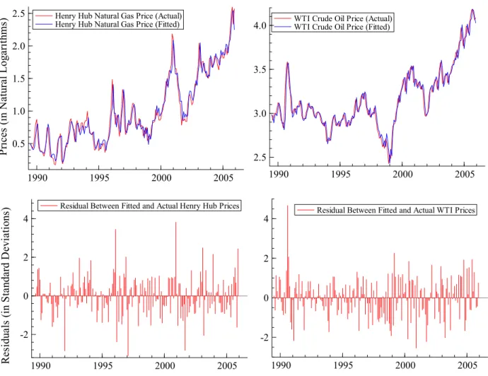
Figures 6 and 7 illustrate these diagnostic properties. Each figure is 2x2 with results for the Henry Hub equation in the left-hand column and the WTI equation in the right-hand column. The actual-fitted diagram is presented in the top row and the scaled residuals are given in the bottom row of Figure 6. The fits for the two price series are close, but there are several large outliers. There appear to be estimated residuals in excess of three standard deviations from the fitted model that can be explained by the occurrence of extraordinary market or geopolitical events. The first is August 1990, when Iraq invaded Kuwait. Oil prices shot up on news of the invasion, as fears that war in the Middle East could adversely affect oil markets. The second was February (and March) 1996 when extreme cold and uncertainty contributed to a large increase in the Henry Hub natural gas price in February, which was then followed by an offsetting decrease in March. The third is September 2001, when terrorist attacks on the World Trade Center and the

(23)

Pentagon heightened uncertainty throughout the United States and its economy. Figure 7 contains histograms in the top row and autocorrelation functions in the bottom row for the two equations respectively. The failures of the tests for normality appear to be the result of the outliers, not skewness or overly fat tails in the distribution of errors. There does not appear to be significant autocorrelation.

Figure 6. Henry Hub and West Texas Intermediate Prices with Fitted Values and

Residuals from a VAR(2)

1990 1995 2000 2005

0.5 1.0 1.5 2.0 2.5 P ri ces ( in N atu ra l Lo ga ri th ms

) Henry Hub Natural Gas Price (Actual) Henry Hub Natural Gas Price (Fitted)

1990 1995 2000 2005

-2 0 2 4 Re si dua ls ( in S ta nda rd D evi at ions

) Residual Between Fitted and Actual Henry Hub Prices

1990 1995 2000 2005

2.5 3.0 3.5

4.0 WTI Crude Oil Price (Actual) WTI Crude Oil Price (Fitted)

1990 1995 2000 2005

-2 0 2

4 Residual Between Fitted and Actual WTI Prices

(24)

24

Figure 7. Implied Empirical Density and Autocorrelogram and of VAR(2) Residuals

-4 -2 0 2 4

0.1 0.2 0.3 0.4 0.5

P

ro

bab

ili

ty

D

en

sity

Henry Hub Natural Gas Price Fitted Residuals Implied Empirical Distribution Normal Distribution (0, 1)

0 5 10

-0.5 0.0 0.5 1.0

Fitted Residual Autocorrelation Function Fitted Residual Partial Autocorrelation Function

-2 0 2 4 6

0.1 0.2 0.3 0.4

WTI Crude Oil Price Fitted Residuals Implied Empirical Distribution Bormal Distribution (0, 1)

0 5 10

-0.5 0.0 0.5 1.0

Fitted Residual Autocorrelation Function Fitted Residual Partial Autocorrelation Function

Model Stability Tests

The natural gas and oil markets are well known for their volatility. International supply and demand shocks can affect the crude oil markets and domestic relative demand; supply shocks, and weather can affect natural gas markets. Any or all of these events could have contributed to instability or “structural” breaks in the data generating process for the Henry Hub and West Texas Intermediate markets.

The textbook approach to model constancy assumes that the modeler knows the date of a possible structural break in the sample. The model is fitted over the full sample and for the two “halves” of the sample. The full sample implicitly imposes the same model structure throughout and can be considered a restricted model. This is evaluated against the unrestricted model

(25)

comprised of the two “halves” using an F-test. We take an agnostic view on the possibility and timing of structural breaks over the 1989-2005 samples.

Model constancy of the VAR system is evaluated using recursive estimation techniques. Assuming the original model has T observations, the technique begins by estimating the model first over s < T observations in the sample and then fit the model using s + 1, s + 2, ..., up to T observations. At this point there are a number of tests for evaluating model (and parameter) constancy. They are often best presented in graphical form, because of the large number of statistics that are calculated.

A familiar statistical presentation is the 1-step residuals plus the standard error bound used to search for outliers. The 1-step residuals are given by eˆt=yt -xt′

β

ˆ_t and plotted with the current estimate of plus or minus 2

σ

ˆ

t on either side of zero. When eˆ is outside the band it can be t interpreted as an outlier. Standardized innovations are another way to illustrate the presence of outliers.

Two types of recursive Chow tests are reported. The first is the 1-step Chow test. This looks at the sequence of one period ahead prediction from the recursive estimation for period s to T. The tests are F(1,t-k-1) under the null hypothesis of parameter constancy. The statistic is calculated as:

1 1

( ) ( 1)

(1, 1) , 1, ... ,

t t

t

RSS RSS t k

F t k where t s s T

RSS

− −

⎛ − − − ⎞

− − = +

⎜ ⎟

⎝ ⎠ (11)

The test assumes that the dependent variables y_t, are approximately normally distributed.

The N-down test orBreakpoint Chow test plots the test statistic over the sample, scaled by either the 5 percent or 1 percent critical value and, can be interpreted as a forecast stability test. The model is estimated for the first s observations. A forecast is constructed using the estimated coefficients from period s+1 through T and the F-test is calculated. The null hypothesis is that

(26)

26

model is estimated and forecasts are performed recursively. Recursive estimation permits construction of Chow tests over the full sample and lets the data do the talking.

The Breakpoint Chow test is calculated as:

1 1

( ) ( 1)

( 1, 1) , 1, ... ,

/ ( 1)

T t

t

RSS RSS t k

F T s t k where t s s T

RSS T s

− −

⎛ − − − ⎞

− + − − = +

⎜ _{− −} ⎟

⎝ ⎠ (12)

Figure 8. Recursive Chow Tests for Model Stability

1995 2000 2005

1 2 3

1- Step Chow Test 1-Step Ln Henry Hub Natural Gas Price 1-Percent Level of Significance

1995 2000 2005

1 2

1-Step Ln WTI Crude Oil Price 1-Percent Level of Significance

1995 2000 2005

1

2 1-Step Joint Test Statistic 1-Percent Level of Significance

1995 2000 2005

0.50 0.75 1.00

1.25 Breakpoint Chow Test

Breakpoint Ln Henry Hub Natural Gas Price 1-Percent Level of Significance

1995 2000 2005

0.5 1.0

Breakpoint Ln WTI Crude Oil Price 1-Percent Level of Significance

1995 2000 2005

0.75 1.00

1.25 Breakpoint Joint Test Statistic 1-Percent Level of Significance

Note: 1-step Chow tests and the Break-Point Chow tests are reported in the left hand and right-hand columns, respectively.

Note: Tests on Henry Hub natural gas prices and WTI crude oil prices are reported in the first and second rows, respectively. Joint-Chow tests are reported in the bottom row.

Note: Test statistics are scaled on the appropriate critical value at 1-percent levels of significance.

(27)

The results of the 1-step Chow tests and the Break-Point Chow test are presented graphically in Figure 8. They are reported in the left-hand column and right-hand column, respectively. At each observation, the normalized test statistic was calculated as the ratio of the statistic compared with the appropriate critical value at 1 percent. The sequence of tests is plotted. When the normalized value exceeds unity, this indicates a rejection of the null hypothesis of no structural break.

The 1-step Chow test results indicate two large spikes in the Henry Hub equation, both of which are associated with freezing weather in February 1996 and January 2001, respectively. There is a single large spike for the Henry Hub price that occurs in early 2000. This was a period of fairly volatile crude oil prices where prices fell by 15 percent in 1 month and recovered by twice that in the next 3 months. The joint 1-step Chow test reveals that these three observations are significant as well.

The Break-Point Chow tests demonstrate the impact of the freezing weather in 1996 on the Henry Hub equation. Thereafter the stability of the equation of the model settles down. However, in 2005 the equation appears to become less stable, but not significantly. This issue bears further analysis as the model is used in the future. The Henry Hub and system Break-Point tests are affected by the February 1996 spike in natural gas prices and the period mid-1998 through 1999. A possible explanation for this latter result is the forecast of increasing global demand for oil by the Organization of Petroleum Exporting Countries (OPEC) and the increase in quotas leading to a supply glut in the market wherein crude oil prices fell by 50 percent. In addition, crude oil demand fell because of the Asian financial crisis during this period. Otherwise both of these diagrams suggest the equation and system are stable.

The Cointegration Analysis of the Vector Autoregression Model

In this section the Johansen procedure is applied to test for the presence of cointegration (Johansen, (1988), and Hendry, Juselius, (2000)). The VAR model in levels can be linearly transformed into a model that is expressed in first differences.

(28)

28

(

)

,1 1 1 1 ,2 1 1

1 2 1 2

ln ln ln

0, , , .

t

t t t

t

t t t t

HenryHub HenryHub HenryHub constant

B

WTI WTI WTI timetrend

I ε ε ε − − − −

Δ Δ ⎡ ⎤

⎡ ⎤ _{= Γ} ⎡ ⎤_{+ Π}⎡ ⎤₊ ⎡ ⎤

+ ⎢ ⎥ ⎢ _Δ ⎥ ⎢ _Δ ⎥ ⎢ ⎥ ⎢ ⎥

⎣ ⎦ ⎣ ⎦ ⎣ ⎦ ⎣ ⎦ ⎣ ⎦

Ω Γ = −Π Π = Π + Π −

(13)

The crux of the Johansen test is to examine the mathematical properties of the Π matrix in equation (7), which contains important information about the dynamic stability of the system. Intuitively, the Π matrix in equation (13) contains the expression relating the levels of the two endogenous variables, the Henry Hub and WTI spot prices. With two endogenous variables in the VAR, the Π matrix has one linearly independent row, then crude oil and natural gas prices might have a cointegrating relationship. In the specification with two endogenous variables there can be as many as two linearly independent equations or no linearly independent equations.8_The

former implies the two series should be considered as stationary, and the latter implies there is no cointegrating relationship and modeling in first differences is appropriate.

Engle and Granger (1987) demonstrate the one-to-one correspondence between cointegration and error correction models. Cointegrated variables imply an error correction model (ECM) representation for the econometric model and, conversely, models with valid ECMs imply cointegration.

Evaluating the number of linearly independent equations in Π is done by testing for the number of non-zero characteristic roots, or eigenvalues, of the Π matrix, which equals the number of linearly independent rows.9 The matrix can be rewritten as the product of two full column vectors, Π =α β'.

The matrix

β

' is referred to as the cointegrating vector and α as the weighting elements for the corresponding cointegrating relation in each equation of the VAR. The vector

β

'Yt−₁ is normalized on the variable of interest in the cointegrating relation and interpreted as the deviation from the “long-run” cointegrating condition. In this context, the column α represents the speed of adjustment coefficients from the error in each equation. If the coefficient is zero in a

8_{If the rank of}_Π_{is equal to the number of endogenous variables, then all of the original series are stationary;} and if the rank of Πis zero, there are no cointegrating vectors.

(29)

particular equation, that variable is considered to be weakly exogenous and the VAR can be conditioned on that variable.

The α coefficients are interpreted as the speed of adjustment back towards the long-run cointegrating relationship. In addition, their significance is important from a statistical standpoint. When the I(1) variables are expressed in a VAR system in first differences or the error correction form as in equation (3) above, the issue of weak exogeneity (Engle, Hendry, and Richard, (1983)) and model conditioning can be addressed.

Weak exogeneity implies that the β terms or long-run error correction relations do not provide explanatory power in a particular equation. If this is true, then valid inference can be conducted by dropping that equation from the system and estimating a conditional model.

Prior to conducting the test for cointegration, the possibility of deterministic trends in the data, in addition to stochastic trends, must be considered, because the asymptotic distribution of the test statistic used in the cointegration test is sensitive with respect to assumptions about deterministic trends in the data. From Figure 6, the expected values of the differenced prices series appear to be roughly equal to 0. This suggests that there is not a deterministic trend in the differenced series, and so including a trend variable outside of the cointegration relation in the estimation of equation (7) does not appear necessary. However, there may be a deterministic trend within the cointegration relationship, itself. In the lower panel of Figure 2, the Henry Hub series appears to be rising slightly faster than the adjusted WTI series, starting out consistently below the WTI series, until sometime in 1993, and thereafter exceeding the WTI series on a fairly regular basis. To test the possibility of a trend in the cointegrating relation, a trend variable will be restricted to the cointegrating equation. The VAR model in differences from equation (13) can be written as:

,1

1 1 1

1

,2

1 2 1

ln ln ln

'

ln ln ln

t

t t t

t t

t t t

HenryHub HenryHub HenryHub

t B X

WTI WTI WTI

ε α

β μ

ε α

− −

Δ Δ ⎡ ⎤ ⎡ ⎤

⎡ ⎤ ⎡ ⎤ ⎡ ⎤ ⎡ ⎤

= Γ + _⎢ + _⎥+ +_{⎢ ⎥} ⎢ _Δ ⎥ ⎢ _Δ ⎥ ⎢ ⎥ ⎢ ⎥

⎣ ⎦

(30)

30

presented in Table 5. The eigenvalues of the Π matrix are sorted from largest to smallest. The tests are conducted sequentially, first examining the possibility of no cointegrating relation against the alternative that there cointegrating relations, and then the null of one cointegrating relation against the possibility of two cointegrating relations, e.g., the two price series are actually stationary. Essentially, these are tests of whether the eigenvalue(s) is (are) significantly different from zero. Both the Johansen trace test and max test support rejection of the null hypothesis that there are no cointegrating relations in the system. The first row tests the null hypothesis of rank equal to zero. The Trace test and the Max(imum) eigenvalue test are rejected at 1 percent whether the asymptotic or degrees of freedom (T-nm) adjustment is used at 1 percent. However, the Johansen tests are unable to reject the hypothesis that there is more than one cointegrating equation in the second row. These results indicate that there is a single significant cointegration equation in the system, relating the long-run difference between the Henry Hub natural gas and WTI crude oil spot prices.

The next step involves identifying and interpreting the estimated coefficients of the cointegrating relationship. The VAR is re-estimated, restricting it to incorporate only the significant cointegrating equation in the system. From the earlier discussion, the hypothesis is that the Henry Hub natural gas price is related to the WTI price in an error correction relation. Further this relation is important in explaining deviations in the short-run for natural gas prices, but not for the WTI price. This involves testing of the α and β vectors.

The standardized eigenvector, or β vector, is normalized on the Henry Hub price with standard errors reported in the second part of Table 5. The normalization of the natural gas price makes its associated standard error equal 0. The cointegrating relation may be interpreted as expressing the Henry Hub price as a function of the WTI price and a trend term, so that the Henry Hub price is equal to 81 percent of the crude oil price plus a trend term of about 0.52 percent. The signs on the coefficients in the table are expressed in the form of the condition that the error correction relation, a linear function of the I(1), series is stationary and centered on zero. The tests for the statistical significance of the β coefficients are reported as Chi-square tests with 1 degree of freedom. They are individually significant at 1 percent; with test statistics of 12.5 for the LnWTI and 11.8 for the Trend. The joint test that both of the estimated β coefficients are both statistically insignificant is rejected with a test statistic of 26.1 and a p-value of less than 1

(31)

percent.

Table 5. Johansen Cointegration Analysis of Henry Hub Natural Gas Spot Price and West Texas Intermediate Spot Crude Price

Unrestricted Cointegration Rank Tests

Rank Eigenvalue Trace test _{[ Prob]} Max test _{[ Prob]} Trace test _(T-nm) Max test _(T-nm) 0 0.1309 34.36 _[0.003]** _[0.001]** 27.78 _[0.003]**33.66 _[0.002]** 27.22 1 0.0327 6.58 _[0.401] 6.58 _[0.402] 6.45 _[0.417] 6.45 _[0.417]

Standardized Eigenvalues or βs with Standard Errors

lnHenryHub lnWTI Trend

1 -0.81221 -0.00516

0 0.1489 0.00089

Standardized α coefficients with Standard Errors

lnHenryHub lnWTI

-0.231 -0.007

0.043 0.026

Tests for Significance of the β Coefficients Joint Test of the βs

lnWTI Chi^2(1) = 12.494 [0.0004]** Chi^2(1) = 26.188

Trend Chi^2(1) = 11.819 [0.0006]** [0.0000]**

Tests for Weak Exogeneity

lnHenryHub Chi^2(1) = 20.810 [0.0000]**

lnWTI Chi^2(1) = 0.057005 [0.8113]

Note: * , significant at 5 percent; **, significant at 1 percent Source: Energy Information Administration, Natural Gas Division.

Next, hypothesis testing is conducted on the α vector. First, the cointegrating relation is identified by examining itsα , or speed of adjustment, coefficient. It must be negative for the relation to be consistent with a stationary process. The standardized α coefficients and the associated tests for weak exogeneity are found below the β tests. The coefficient for the Henry

(32)

32

coefficient is referred to as checking for weak exogeneity. This determines whether the cointegrating relation can explain changes in the particular series. In this case we are testing if the changes in the WTI are influenced or explained by the cointegrating relation. The coefficient for the WTI is small, -0.007, relative to its standard error, 0.026, and a chi-square statistic of 0.057 with p-value of 0.81. This suggests that the cointegrating relation does not have significant explanatory power on the evolution of the WTI price. However, the cointegrating relation is highly significant for the Henry Hub price equation.

These results are consistent with a cointegrating relation, which can be referred to as an error correction mechanism (ECM). This is expressed as:

0.8122ECMt = LnHenryHubt − ×LnWTIt −0.0051×Trend (15) The ECM at each observation can be interpreted as depicting departures from a long-run equilibrium. The trend term captures a combination of the relative demand and supply factors and may reflect factors that affect the interrelationship between these fuel markets. One explanation for the time trend term may be the fundamental changes to the natural gas market caused by regulatory reform that occurred shortly before and during the period of estimation. These issues are beyond the scope of the current analysis; however, they may be addressed in a future study.

Figure 9 provides an illustration of the ECM. The zero-line indicates that ECM is equal to zero, and the plotted line shows the deviations between the actual Henry Hub natural gas price and that predicted by the WTI crude oil price and the trend component. A shock to crude oil or natural gas prices is followed by an adjustment in the Henry Hub price until the ECM returns to zero. For example, the peak in February 1996 shows the impact of the severe cold weather nationwide on natural gas prices as the Henry Hub price climbed to $4.42 per MMBtu compared with the preceding month’s price of $2.92 per MMBtu. Similarly, the peak in December 2000 also shows the impact of severe freezing weather as Henry Hub prices rose from $5.52 per MMBtu in November to $8.90 per MMBtu in December. In each case these departures zero were eventually followed by the ECM returning to the zero-line.

(33)

Figure 9. The Estimated Cointegrating Vector, Error Correction Mechanism, Between Henry Hub and WTI Prices (1989-2005)

1990 1995 2000 2005

-0.6 -0.4 -0.2 0.0 0.2 0.4 0.6

Er

ro

r C

or

rectio

n M

ech

an

is

m

Cointegrating Relation

The Conditional Error Correction Model

The two equation system can be reduced to a single conditional error correction model. WTI prices were found to be weakly exogenous. A conditional model means the original model (or system) has been partitioned into a subset. Weak exogeneity of the WTI price implies that for inference purposes only the change or first differences of the Henry Hub equation needs to be estimated. Similar to the VAR approach, the ECM starts from a general form and is reduced to a final model. The VAR analysis was used to examine the long-run relation between the two prices. When examining the relationship in the short run other factors may have important explanatory power so they are included in the model (equation). These additional factors influence only the short-run movements in prices not the long-run. The general equation can be

(34)

34

( )

3 3

0 1

1 0

'

t i t i j t j ECM t

i j

t t t t t

LnHH LnHH LnWTI ECM

Shifts and Outliers Centered Seasonals L X

α γ η α

σ ω ε

− − −

= =

Δ = + Δ + Δ +

+ + + Φ +

∑

₍₁₆₎

The first three expressions contain three lags of the dependent variable, the current and three lags of the change in the WTI, and the lagged ECM term. The next expression represents more “permanent” impacts on the market caused by shifting from a “gas bubble” environment to tighter supplies, as in the late 1990s and the onset of tight supplies in the oil markets pushing up natural gas prices. These effects are captured in deterministic variables for outliers and shifts. The next expression contains the seasonal factors that have short-run effects on natural gas prices. The last components, Xt, include variables which are thought to help explain short-run

movements in the Henry Hub price. The Φ

( )

L expression represents a lag polynomial operator for the matrix of these variables. It includes the contemporaneous values of these variables and their lags for each month. The variables are working inventories of natural gas and weather variables like heating degree days. Monthly working inventories and their levels relative to the minimum over the past 5 years are often used in analyses of the short-run movements of natural gas prices. Increases in inventories (relative to minimums) reflect slackness in the market. Thus, they should have a negative effect on price changes. Heating degree days and their deviations from 30-year norms are important factors as well. Cold weather increases the demand for heating from natural gas and puts upward pressure on its price. In several months it was noted earlier that there might be outliers as a result of heavy storms and market interruptions.

The general error correction equation contained 32 estimated coefficients. Once again, the objective is to ensure that the data process for the change in WTI is explained such that the last part, the residual disturbance term is a white noise process. We follow a general to specific approach of testing reductions on this equation to find a congruent model.

Empirical models are at best approximations of the true data generating process (DGP). The econometric model should exhibit certain desirable properties that render it a valid representation of the true DGP. Hendry (1995) and Mizon (1995) suggest the following six criteria according to the London School of Economics (LSE) methodology.

(35)

1. There are identifiable structures in the empirical model that are interpretable in light of economic theory.

2. The residuals must be white noise for the model to be a valid simplification of the DGP. 3. The empirical model must be admissible on accurate observations. For example, nominal

interest rates and prices cannot be negative.

4. The conditioning variables are at least weakly exogenous for the parameters of interest in the model. Forecasting models require strong exogeneity, while policy models require super exogeneity.

5. The parameters of interest must be constant over time and remain invariant to certain classes of interventions. This relates to the purpose of the model in the previous criteria. 6. The model must be able to explain the results from rival models; it is able to encompass

them.

The general to specific model reduction process follows diagnostic tests of comparing the model fit from restrictions on lags at different lags, blocks of variables, transformations of variables. We used the econometric software, PcGets, developed by David Hendry and Hans-Martin Krolzig (2001), and searched all the possible paths in reducing the model to a final model. The final specification and estimation of the model may be expressed as:

1 1

0.25 0.26 0.14 0.19

t t t t t t

HH WTI HH₋ ECM ₋ Bx ε

Δ = − + Δ + Δ − + + (17)

Where Β and xt are matrices of estimated parameters and associated exogenous short-run effects, respectively.

Estimating the model using the LSE general to specific reduction approach has the benefit of increased simplicity in more ways than one. Because crude oil prices are now treated as an exogenous variable, the impulse dummy variable for August 1990 may now be dropped from the model. Tests of exclusion were conducted on each of the remaining deterministic variables, including the impulse dummy variables. Outlier dummy variables for December and February 1997, and September 2001, as well as the transitory dummy variable for February/March 1996 and February/March 2003 were necessary to ensure multivariate normality and