The Singular Value Decomposition in Symmetric (Löwdin) Orthogonalization and Data Compression

The Singular Value Decomposition in

Symmetric (L¨

owdin) Orthogonalization

and Data Compression

The SVD is the most generally applicable of the orthogonal-diagonal-orthogonal type matrix decompositions

Every matrix, even nonsquare, has an SVD

The SVD contains a great deal of information and is very useful as a theoretical and practical tool

*******************************************************************

1 Preliminaries

Unless otherwise indicated, all vectors are column vectors

u ∈ Rn =⇒ u =

    

u1

u2

... un

     ∈ R

Definition 1.1 Let u ∈ Rn, so that u = (u1, u2, . . . un)T. The (Euclidean) norm

of u is defined as

kuk₂ =

q

u2₁+u2₂ +· · ·+u2

n = n X

j=1

u2_j

!1/2

Definition 1.2 A vector u ∈ Rn is a unit vector or normalized if

kuk₂ = 1

===========================================

Definition 1.3 Let A = (aij) ∈ Rm×n. The transpose AT of A is the matrix

(aji) ∈ Rn×m.

===========================================

Example 1.4

1 0 3

2 −1 −4

T

=

 

1 2

0 −1 3 −4

 

Definition 1.5 (Matrix Multiplication) Let A ∈ Rm×n, B ∈ Rn×p. Then the product AB is defined element-wise as

(AB)ij = n X

k=1

aikbkj

and the matrix AB ∈ Rm×p

===========================================

Definition 1.6 Let u, v ∈ Rn. Then the inner product of u and v, written hu, vi

is defined as

hu, vi =

n X

j=1

ujvj =uTv

===========================================

Note that this notation permits us to write matrix multiplication as entry-wise inner products of the rows and columns of the matrices

===========================================

If we denote the ith row of A by iA and the jth column of B by Bj we have

Example 1.7

−1 1 0

3 −2 1





2 3

0 −2 6 −3

 

=

 

−1·(2) + 1·(0) + 0·(6) −1 ·(3) + 1·(−2) + 0·(−3) 3·(2) +−2 ·(0) + 1·(6) 3·(3) +−2 ·(−2) + 1·(−3)

 

=

−2 −5 12 10

===========================================

Definition 1.8 Two vectors u, v ∈ Rn are orthogonal if

hu , vi = uTv = u1 u2 · · · un

    

v1

v2

... vn

    

= u1v1+u2v2 +· · ·+unvn = 0

===========================================

Recall that the n-dimensional identity matrix is

In =     

1 0 · · · 0

0 1 ...

... . . .

0 · · · 1

    

We’ll write I for the identity matrix when the size is clear from the context.

===========================================

Definition 1.9 A square matrix Q∈ Rn×n is orthogonal if QTQ= I.

===========================================

This definition means that the columns of an orthogonal matrix A are mutually orthogonal unit vectors in Rn

===========================================

Alternatively, the columns of A are an orthonormal basis for Rn

===========================================

But since matrix multiplication is associative, QT is the right-inverse (and hence the inverse) of Q - indeed, let P be a right-inverse of Q (so that QP = I); then

(QTQ)P =QT(QP) ⇐⇒ IP = QTI ⇐⇒ P =QT

===========================================

The SVD is applicable to even nonsquare matrices with complex entries, but for clarity we will restrict our initial treatment to real square matrices

*******************************************************************

2 Structure of the SVD

Definition 2.1 Let A ∈ Rn×n. Then the (full) singular value decomposition of A is

A =UΣVT =

          

U1 U2 · · · Um                      

σ1 0 · · · 0

0 σ2 · · · 0

... . . . 0

0 · · · σn

0 · · · 0

... ...

0 · · · 0

                

(V1)T

(V2)T

... (Vn)T

      .

where U, V are orthogonal matrices and Σ is diagonal

The σi’s are the singular values of A, by convention arranged in nonincreasing

order

σ1 ≥ σ2 ≥ · · · ≥σn ≥ 0;

Since U and V are orthogonal matrices, the columns of each form orthonormal (mutually orthogonal, all of length 1) bases for Rn

===========================================

We can use these bases to illuminate the fundamental property of the SVD:

===========================================

For the equation Ax = b, the SVD makes every matrix diagonal by selecting the right bases for the range and domain

===========================================

Let b, x ∈ Rn such that Ax = b, and expand b in the columns of U and x in the columns of V to get

Then we have

b = Ax ⇐⇒ UTb = UTAx

= UT(UΣVT)x = (UTU)Σ(VTx) = IΣx0

= Σx0

or

b = Ax ⇐⇒ b0 = Σx0

===========================================

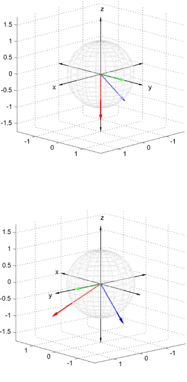
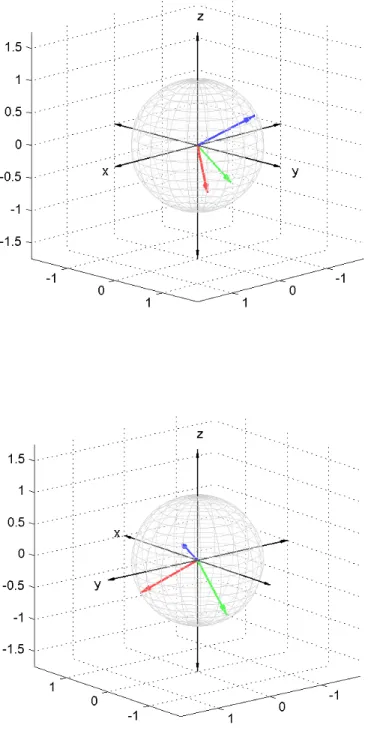
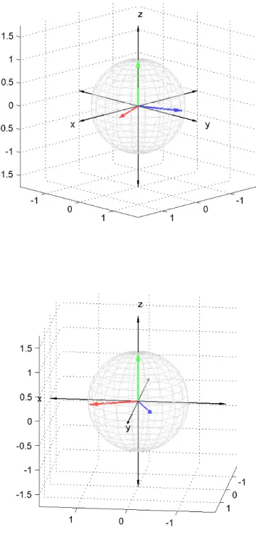
Let y ∈ Rn, then the action of left multiplication of y by A (computing z = Ay) is decomposed by the SVD into three steps

z = Ay

= (UΣVT)y = UΣ(VTy) = UΣc (c := VTy)

c =VTy is the analysis step, in which the components of y, in the basis of Rn given by the columns of V, are computed

===========================================

w = Σc is the scaling step in which the components ci, i ∈ {1,2, . . . , n} are

dilated

===========================================

z = U w is the synthesis step, in which z is assembled by scaling each of the Rn-basis vectors ui by wi and summing

So how do we find the matrices U,Σ, and V in the SVD of some A ∈ Rn×n?

===========================================

Since VTV = I =UTU, A =UΣVT yields

AV = UΣ and (1)

UTA = ΣVT or, taking transposes

ATU = VΣ (2)

===========================================

Or, for each j ∈ {1,2, . . . , n},

Avj = σjuj from Equation 1 (3)

ATuj = σjvj from Equation 2 (4)

===========================================

ATAvj = ATσjuj

= σjATuj

= σ_j2vj

===========================================

So the vj’s are the eigenvectors of ATA with corresponding eigenvalues σ_j2

===========================================

Note that (ATA)ij = iAAj or

ATA=

          

1AA1 1AA2 · · · 1AAn

2AA1 2AA2 ...

... . ..

nAA1 · · · nAAn

          

(5)

ATA is a matrix of inner products of columns of A - often called the Gram matrix of A

Let’s do an example:

A=

 

1 0 −1 1 1 0

−1 0 −1



 =⇒ AT =

 

1 1 −1 0 1 0

−1 0 −1

 

=⇒ ATA =

 

3 1 0 1 1 0 0 0 2

 

===========================================

To find the eigenvectors v and the corresponding eigenvalues λ for B := ATA, we solve

Bx =λx ⇐⇒ (B −λI)x = 0

The standard technique for finding such λ and v is to first note that we are looking for the λ that make the matrix

B −λI =

 

3 1 0 1 1 0 0 0 2

 −

 

λ 0 0 0 λ 0 0 0 λ

  =

 

3−λ 1 0

1 1−λ 0

0 0 2−λ

 

singular

===========================================

This is most easily done by solving det(B −λI) = 0 :

3−λ 1 0

1 1−λ 0

0 0 2−λ

= (3

−λ)(1−λ)(2−λ) −2 +λ

= −λ3+ 6λ2−10λ + 4 = 0

⇐⇒

σ₁2 = λ1 = 2 +

√

2

σ₂2 = λ2 = 2

σ₃2 = λ3 = 2−

√

Now (for a gentle first step) we’ll find a vector v2 so that ATAv2 = 2v2

===========================================

We do this by finding a basis for the nullspace of

ATA−2I =

 

3−2 1 0

1 1 −2 0

0 0 2 −2



 =

 

1 1 0 1 −1 0 0 0 0

 

===========================================

Certainly any vector of the form

 

0 0 t



, t ∈ R, is mapped to zero by

ATA−2I

===========================================

So we can set v2 =

 

0 0 1

 

To find v1 we find a basis for the nullspace of

ATA−(2 +

√ 2)I =   1 − √

2 1 0

1 −1− √

2 0

0 0 −

√

2

 

which row-reduces ( R2 ←− (1 +

√

2)R1 +R2, then R3 ←→ R2 ) to

 

1 − √

2 1 0

0 0 − √

2

0 0 0

 

===========================================

So any vector of the form

      s (−1 +

√ 2)s 0     

 is mapped to zero by

ATA−(2 +

√

2)I

===========================================

so v₁0 =

      1

−1 +

√ 2      

So we set v1 =

v₁0

kv0

1k

= _p 1 4−2

√ 2       1

−1 +

√ 2 0       ===========================================

We could find v3 in a similar manner, but in this particular case there’s a

quicker way...

===========================================

v3 =

     

−(v1)2

(v1)1

0       = 1 p

4−2

√ 2       1− √ 2 1 0      

Certainly v3 ⊥ v2 and by construction v3 ⊥v1 - recall the theorem from linear

We’ve found V =     

 v1 v2 v3       =         1 √

4−2

√ 2 0 1− √ 2 √

4−2

√

2

−1+√2

√

4−2

√

2 0

1

√

4−2

√

2

0 1 0

        ===========================================

And of course

Σ =        p 2 + √

2 0 0

0 √2 0

0 0 p2 −√2

       ===========================================

If σn > 0, Σ is invertible and

U =AVΣ−1

===========================================

So we have

U =      

1 0 −1

1 1 0

−1 0 −1

              1 √

4−2√2 0

1−√2

√

4−2√2

−1+

√

2

√

4−2

√

2 0

1

√

4−2

√

2

0 1 0

                1 √

2+√2 0 0

0 √1

2 0

0 0 √ 1

2−√2

        =      

1 0 −1

1 1 0

−1 0 −1

             1

2 0 −

1 2

−1+√2

2 0

1 2(

√

2−1)

0 √1

2 0        =        1 2 − 1 √ 2 − 1 2 1 √ 2 0 1 √ 2

1 1 1

      

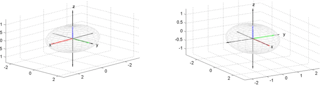
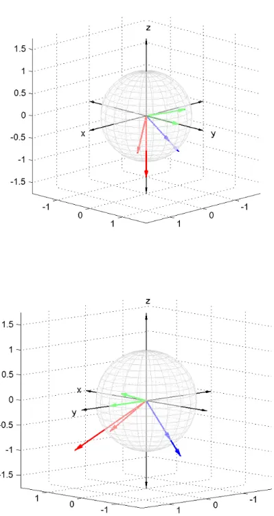
Figure 4: The columns ofΣin the ellipse formed by Σacting on the unit sphere by left-multiplication

Figure 5: The columns ofAV =UΣin the ellipse formed byAacting on the unit sphere by left-multiplication

===========================================

Note that the columns of U and V are orthogonal (as are, of course, the columns of Σ)

Note that in practice, the SVD is computed more efficiently than by the direct method we used here; usually by (OK, get ready for the gratuitous mathspeak)

reducing A to bidiagonal form U1BV1T by elementary reflectors or Givens

ro-tations and

directly computing the SVD of B (=U2ΣV2T)

then the SVD of A is (U1U2) Σ (V2T V1T )

===========================================

If σn = 0, then A is singular and the entire process above must be modified

slightly but carefully.

===========================================

If r is the rank of A (the number of nonzero rows of the row-echelon form of A) then

n−r singular values of A are zero (equivalently if there are n−r zero rows in the row-echelon form of A), so

Σ−1 is not defined, and we define the pseudo-inverse Σ+ of Σ as Σ+ =diag(σ₁−1, σ₂−1, . . . , σ−_r1, 0, . . . , 0)

Thus we can define the first r columns of U via AVΣ+ and to complete U we choose any n−r orthonormal vectors which are also orthogonal to

span{u1, u2, . . . , ur}, via, for example, Gram-Schmidt

===========================================

Recall that the SVD is defined for even nonsquare matrices

===========================================

In this case, the above process is modified to permit U and V to have different sizes

===========================================

If A ∈ Rm×n, then

U ∈ Rm×m

Σ ∈ Rm×n V ∈ Rn×n

In the case m > n : A =           

a11 a12 · · · a1n

a21 a22 · · · a2n

... . . . ... am1 · · · amn

           =           

u11 u12 · · · u1n · · · u1m

u21 u22 · · · u2n · · · u2m

... . . . ... um1 · · · umn · · · umm

                     

σ1 0 · · · 0

0 σ2 · · · 0

... . . . 0

0 · · · σn

0 · · · 0

... ...

0 · · · 0

               

v11 v12 · · · v1n

v21 v22 ...

... . . . vn1 · · · vnn

    

or, in another incarnation of the SVD (the reduced SVD)

A =           

u11 u12 · · · u1n

u21 u22 ...

... . . .

um1 · · · umn

               

σ1 0 · · · 0

0 σ2 · · · 0

... . . . ...

0 · · · σn

         

v11 v12 · · · v1n

v21 v22 ...

... . .. vn1 · · · vnn

    

where the matrix U is no longer square (so it can’t be orthogonal) but still has orthonormal columns

If m < n: A =     

a11 a12 · · · a1m · · · a1n

a21 a22 · · · a2n

... . . . ...

am1 · · · amn

     =     

u11 u12 · · · u1n

u21 u22 ...

... . . . un1 · · · unn

     ×     

σ1 0 · · · 0 0 · · · 0

0 σ2 · · · 0 0 · · · 0

... . . . ... ... 0 · · · σn 0 · · · 0

     ×               

v11 v12 · · · v1n · · · v1m

v21 v22 · · · v2n · · · v2m

... . . . ... vn1 vn2 · · · vnn · · · vnm

... . . . ... vm1 · · · vmn · · · vmm

              

In which case the reduced SVD is

A =

    

u11 u12 · · · u1n

u21 u22 ...

... . . . un1 · · · unn

    

    

σ1 0 · · · 0

0 σ2 · · · 0

... . . . ...

0 · · · σn

    

    

v11 v12 · · · v1n · · · v1m

v21 v22 · · · v2n · · · v2m

... . . . ... vn1 vn2 · · · vnn · · · vnm

    

*******************************************************************

3 Properties of the SVD

Recall r is the rank of A; the number of nonzero singular values of A

===========================================

range (A) = span {u1, u2, . . . , ur}

range (AT) = span {v1, v2, . . . , vr}

null (A) = span {vr+1, vr+2, . . . , vn}

For A ∈ Rn×n, |det A| =

n Y i=1

σi

===========================================

The SVD of an m×n matrix A leads to an easy proof that the image of the unit sphere Sn−1 under left-multiplication by A is a hyperellipse with semimajor

axes of length σ1, σ2, . . . , σn

===========================================

The condition number of an m×n matrix A, with m ≥ n, is κ(A) = σ1

σn

Used in numerics, κ(A) is a measure of how close A is to being singular with respect to floating-point computation

===========================================

The 2-norm of A is kAk₂ := sup

kAxk₂

kxk2 = 1

The Frobenius norm of A is kAk_F :=

m X_Xn

a2_ij

We have

kAk₂ =σ1 and kAkF = q

σ₁2+σ2₂ + · · · +σ2

n

since both matrix norms are invariant under orthogonal transformations (multiplication by orthogonal matrices)

===========================================

Note that although the singular values of A are uniquely determined, the left and right singular vectors are only determined up to a sequence of sign choices

for the columns of either U or V

===========================================

So the SVD is not generally unique, there are 2(maxm,n) possible SVD’s for a given matrix A

===========================================

If we fix signs for, say, column 1 of V, then the sign for column 1 of U is determined - recall AV =UΣ

4 Symmetric Orthogonalization

For nonsingular A, the matrix L := U VT is called the symmetric orthogonalization of the matrix A

===========================================

L is unique since any sequence of sign choices for the columns of V determines a sequence of signs for the columns of U

===========================================

Lij = Ui1(VT)1j +Ui2(VT)2j +Ui3(VT)3j + · · · +Uin(VT)ni

= Ui1Vj1+Ui2Vj2 +Ui3Vj3 + · · · +UinVjn

===========================================

Like Gram-Schmidt orthogonalization, it takes as input a linearly independent set (the columns of A) and outputs an orthonormal set

(Classical) Gram-Schmidt is unstable due to repeated subtractions; Modifed Gram-Schmidt remedies this

===========================================

But occasionally we want to disturb the original set of vectors as little as possible

===========================================

Theorem 4.1 Over all orthogonal matrices Q, ,kA − Qk_F is minimized when Q =L.

5 Applications of the SVD

Symmetric Orthogonalization was invented by a Swedish chemist, Per-Olov L¨owdin, for the purpose of orthogonalizing hybrid electron orbitals

===========================================

Also has application in 4G wireless communication standard, Orthogonal Frequency-Division Multiplexing (OFDM)

===========================================

Nonorthogonal carrier waves with ideal properties, good time-frequency localization, orthogonalized in this manner have maximal TF-localization among

all orthogonal carriers

===========================================

Carrier waves are continuous (complex-valued) functions and not matrices, but there is an inner product defined for pairs of carrier waves via integration

===========================================

With that inner product, the Gram matrix of the set of carrier waves can be computed

The symmetrically orthogonalized Gram matrix is then used to provide coefficients for linear combinations of the carrier waves

===========================================

These linear combinations are orthogonal (hence suitable for OFDM) and optimally TF-localized

===========================================

The SVD also has a natural application to finding the least squares solution to Ax =b (i.e., a vector x with minimal kAx−bk₂) where Ax= b is inconsistent

(e.g., A ∈ Rm×n, m > n , r =n)

===========================================

But perhaps the most visually striking property of the SVD comes from an application in image compression

We can rewrite Σ as     

σ1 0 · · · 0

0 σ2 ...

... . . .

0 · · · σn

     =     

σ1 0 · · · 0

0 0 ...

... . . .

0 · · · 0

    

| {z }

Σ1 +     

0 0 · · · 0

0 σ2 ...

... . . .

0 · · · 0

    

| {z }

Σ2 + . . . +     

0 0 · · · 0

0 0 ...

... . . .

0 · · · σn

    

| {z }

Σn

= Σ1 + Σ2 + · · · + Σn

===========================================

Now consider the SVD

A =     

 U1 U2

· · · Un      

Σ1 + Σ2 + · · · + Σn      

(V1)T

(V2)T

... (Vn)T

     

and focus on, say, the first term      

U1 U2 · · · Un       Σ1      

(V1)T

(V2)T

... (Vn)T

      =      

σ1U1 0 · · · 0

           

(V1)T

(V2)T

... (Vn)T

      =     

 σ1U1 0

· · · 0

           

(V1)T

0 ... 0      

= σ1U1(V1)T

In general UΣkVT =σkUk(Vk)T

So A =

n X

j=1

In this representation of A, we can consider partial sums

===========================================

For any k with 1 ≤ k ≤n, define

A(k) =

k X

j=1

σjUj(Vj)T

===========================================

This amounts to discarding the smallest n−k singular values and their corresponding singular vectors, and storing only the Vj’s and the sjUj’s

===========================================

Theorem 5.1 Among all rank-kmatricesP, kA−Pk_F is minimized for P = A(k)

===========================================

Theorem 5.1 says that the kth partial sum of A(n) captures as much of the “energy” of A as possible

Example Consider the 320-by-200-pixel image below

This is stored as a 320 ×200 matrix of grayscale values, between 0 (black) and 1 (white), denoted by Aclown

===========================================

By Theorem 5.1, A(_clownk) is the best rank-k approximation to Aclown, measured by the Frobenius norm

===========================================

Storage required for A(_clownk) is a total of (320 + 200) ·k bytes for storing σ1u1

through σkuk and v1 through vk

===========================================

320·200 = 64,000 bytes required to store Aclown explicitly

===========================================

Now consider the rank-20 approximation to the original image, and the difference between the images

The original image took 64 kb, while the low-rank approximation required (320 + 200) ·20 = 10.4 kb, a compression ratio of .1625

===========================================

The SVD can also make you rich - but that’s a topic for another time...

===========================================

For further investigation, see

“Numerical Linear Algebra” by Trefethen

“Applied Numerical Linear Algebra” by Demmel “Matrix Analysis” by Horn and Johnson