Feature Sensitive Surface Extraction from Volume Data
Leif P. Kobbelt Mario Botsch
Computer Graphics Group, RWTH-Aachen
Ulrich Schwanecke Hans-Peter Seidel
Computer Graphics Group, MPI Saarbrücken
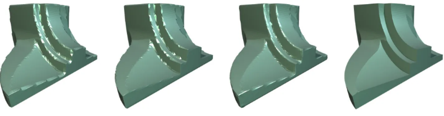
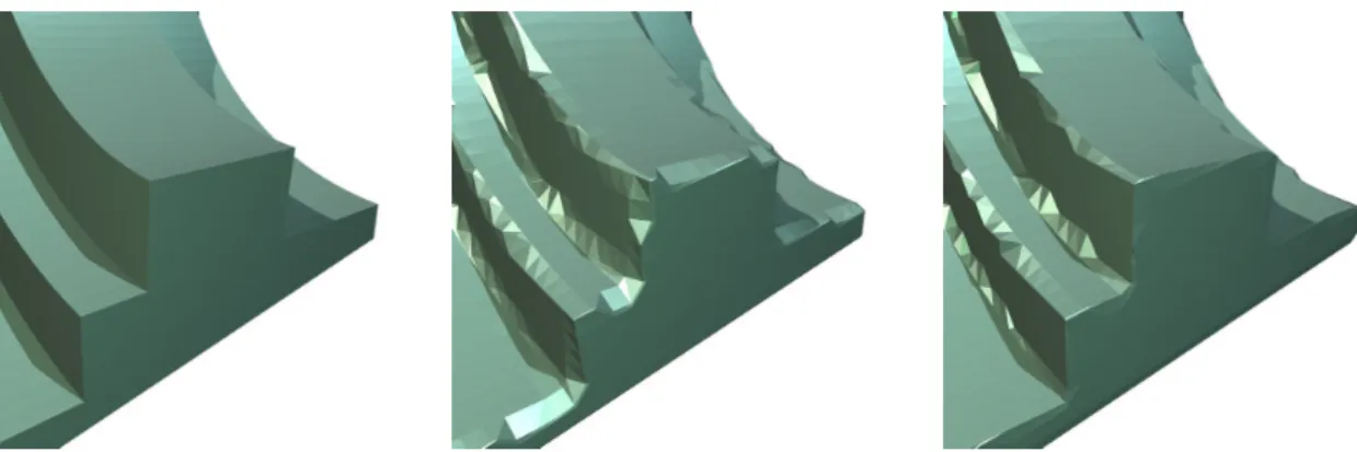
Figure 1: We present a new technique to extract high quality triangle meshes from volume representations of geometric objects. The two main contributions are an enhanced distance field representation and an extended Marching Cubes algorithm. The above figures show reconstructions of the well-known “fandisk” dataset from its distance field representation. The distance field has been sampled on a uniform 65×65×65 grid. The far left image shows the standard Marching Cubes reconstruction, center left is the reconstruction by the same algorithm but applied to the enhanced distance field with the same resolution. Center right shows the result of our new extended Marching Cubes algorithm applied to the original volume data, and finally on the far right we show the reconstruction by our new algorithm applied to the enhanced distance field. The approximation error to the original polygonal model is below 0.25 %.
Abstract
The representation of geometric objects based on volumetric data structures has advantages in many geometry processing applica-tions that require, e.g., fast surface interrogation or boolean opera-tions such as intersection and union. However, surface based algo-rithms like shape optimization (fairing) or freeform modeling often need a topological manifold representation where neighborhood in-formation within the surface is explicitly available. Consequently, it is necessary to find effective conversion algorithms to generate explicit surface descriptions for the geometry which is implicitly defined by a volumetric data set. Since volume data is usually sam-pled on a regular grid with a given step width, we often observe severe alias artifacts at sharp features on the extracted surfaces. In this paper we present a new technique for surface extraction that performs feature sensitive sampling and thus reduces these alias ef-fects while keeping the simple algorithmic structure of the standard Marching Cubes algorithm. We demonstrate the effectiveness of the new technique with a number of application examples ranging from CSG modeling and simulation to surface reconstruction and remeshing of polygonal models.
1
Introduction
There are two major classes of surface representations in computer graphics: parametric surfaces and implicit surfaces. A paramet-ric surface is usually given by a function f that maps some 2-dimensional (maybe non-planar) parameter domainΩinto 3-space while an implicit surface typically comes as the zero-level iso-surface of a 3-dimensional scalar field f(x,y,z)(volume
represen-tation). From an abstract point of view, parametric surfaces are
defined as the range of a function and implicit surfaces are defined as the kernel of a function. Therefore, some operations are much easier to perform on either representation.
For parametric surfaces, e.g., it is very easy to enumerate points on the surface by evaluating the function f at different parameter values in the domainΩ. Neighboring or ”geodesicly” nearby sam-ples p1=f(u1,v1)and p2=f(u2,v2)can be identified by measuring
the differences of the corresponding parameter values(u1,v1)and
(u2,v2). However, given a point p in 3-space it is not that easy to check if this point lies on the parametric surface or not. On the other hand, checking if a given point p lies on an implicit surface is trivial since we just have to evaluate f(p). However, enumerating points on an implicit surface is not straightforward.
The choice of the best suited surface representation consequently depends on the expected operation profile in a specific application. Nevertheless, to obtain maximum flexibility, it is necessary to de-velop algorithms for the conversion between both representations. Conversion from parametric to implicit requires to compute the sur-face’s distance field [25] while conversion from implicit to paramet-ric is usually done by finding surface samples and connecting them to a polygonal mesh [3, 39]. Higher order parametric representa-tions such as NURBS are usually constructed in a second step by surface fitting techniques [18].
the volume representation of an object to the polygonal mesh rep-resentation of its surface. The surface extraction algorithm is an extension of the well-known Marching Cubes algorithm [21] with an enhanced quality of the output mesh.
The major motivation for the development of the new technique are the severe alias artifacts that can be observed at sharp features of the converted surfaces. These artifacts are due to the fact that Marching-Cubes-type algorithms process discrete volume data and the sampling of the implicit surface f(x,y,z,) =0 is performed on the basis of a uniform spatial grid. Figure 1 shows the effect on a CAD example. In a preprocess we converted the well-known ”fan-disk” model into a volume representation by evaluating its distance field on a uniform 65×65×65 grid. When converting the implicit representation back to a polygonal mesh by using the standard MC algorithm, the reconstruction near the sharp features is very bad (far left image in Fig. 1). The size of these artifacts could be re-duced by refinement of the underlying 3D grid but the basic alias problem will not be solved since the surface normals of the recon-structed mesh will not converge to the normal field of the original 3D model.
The central contributions of this paper are:
•We propose an enhanced representation of the discrete distance field: Instead of using a scalar distance value for each grid point of a uniform spatial grid, we store
directed distances in x, y, and z direction. This allows us
to find more accurate surface samples compared to the approximate samples obtained by linear interpolation of the grid values. As it turns out, the generation and han-dling of directed distance fields is no more complicated that the processing of scalar distance fields.
•We present an Extended Marching Cubes algorithm that detects those grid cells through which a sharp fea-ture (edge or corner) of the considered surface passes. Based on the local distance field information and its gra-dient, additional sample points lying on the feature are computed and inserted into the mesh. Consequently we obtain a noticeably improved approximation of the un-derlying surface (cf. Fig. 1) with significantly reduced alias and the guarantee that the surface normals of the approximation quickly converge to the original surface’s normals. The necessary gradient information can be sampled from the original distance field or estimated from a tri-linear interpolant.
The algorithmic structure of the extraction algorithm is identical to the original Marching Cubes algorithm, i.e., every cell of the discrete distance field is processed separately and a surface patch is generated based on local criteria only. The collection of these small pieces eventually yields a triangle mesh approximation of the complete surface.
Both components can be used independently to improve the sur-face extraction, i.e., standard Marching Cubes applied to the en-hanced distance field representation as well as the extended March-ing Cubes applied to standard distance fields both improve the qual-ity of the resulting mesh to a certain degree. The best results are obtained if both components are combined (cf. Fig. 1).
We will start with a brief overview of related work in the con-text of polygonal surface extraction from volume data. In Section 3 we will then motivate and justify our alternative representation of the distance field function which eliminates the approximation er-ror that is introduced by sampling a piecewise tri-linear function instead of the original distance field. In Section 4 we explain the details of our extended Marching Cubes algorithm that generates a feature sensitive triangle mesh approximation by taking the local gradient of the distance field into account. Eventually, in Section 5 we will show a number of applications that demonstrate the effec-tiveness of our algorithm. The examples include the generation of high quality triangle mesh models for implicitly defined CSG ob-jects, the simulation of milling processes, the surface reconstruction
from scattered point clouds and the remeshing of polygonal mesh models. The variety of applications indicates the flexibility of the algorithm.
2
Related work
The basic concept behind volume representations for geometric models is that they characterize the whole space enclosing an ob-ject. By this they are independent from the actual surface topology and this is why volume representations are preferred in applications where the topology of an object can be complicated or even changes during an operation.
There are different conceptual frameworks for volume-based (implicit) surface representations, among them are algebraic sur-faces [4], radial basis functions [42] and voxelizations [5, 15, 22]. In any case, a surface S is represented as the zero-level iso-surface of a scalar valued function f : IR3→IR. To efficiently process vol-ume representations, one generates a discrete approximation of the continuous scalar field f by sampling the function on a sufficiently fine spatial grid gi,j,k.
In the area of volume graphics [13, 15, 26, 34], techniques have been investigated to use volume representations as a univer-sal graphics primitive and to visualize and modify such representa-tions directly without intermediate conversion. However, in many geometric modeling and processing applications, explicit surface representations are necessary to satisfy the geometric quality re-quirements and to provide direct access to inherent surface prop-erties such as the geodesic neighborhood relation and differential geometric characteristics (e.g. curvatures). Consequently, much ef-fort has been spend to develop efficient and flexible algorithms for the extraction of explicit surface information from volume datasets. Two subproblems have to be solved in this context: first, find a dense set of surface samples and then connect them in a topologi-cally consistent manner to obtain a sufficiently close approximation of the original surface S. In general we distinguish between grid-based techniques and grid-less techniques.
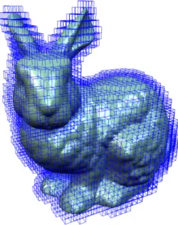
Figure 2: The adaptive octree refinement yields a set of finest-level cells whose union completely contains the surface S. Any algorithm applied to the volume representation of the surface can be restricted to these cells.
Grid-less techniques start with some initial polygonal mesh ap-proximation of the surface S that is iteratively improved by
attract-ing the mesh vertices to the surface S. The scalar field f serves as a potential field to guide the movement of the vertices. Since this
attracting force acting on the mesh vertices can be combined with
a regularizing force which tends to improve the aspect ratio of the triangles, grid-less techniques usually lead to high quality meshes if the underlying surface S is smooth [23, 30, 40, 43]. However, in the presence of sharp features in the surface, alias effects become vis-ible which are partially due to the finite discretization of the scalar field f but also due to the fact that mesh vertices are not explicitly attracted to those features (and hence vertices hit the features only statistically).
The grid-based techniques extract a piece of the surface S for each cubic cell in the grid gi,j,k. Surface samples are computed by
(approximate) intersection of the cell edges with the surface and a triangle mesh is generated that connects these samples. Most grid-based techniques are conceptually derived from the Marching
Cubes algorithm [21] where a pre-processed triangulation is stored
in a table for all possible configurations of edge intersections. Many variants of this basic algorithm have been published which resolve ambiguities [32, 33] or suggest alternative ways to approximate the surface samples [31].
Since the complexity of the uniform grid gi,j,kincreases cubi-cally, with decreasing step width h, one often adapts the sampling density to the local geometric significance in the scalar field f . Hi-erarchical sampling schemes like the octree technique start with a very coarse root cell. This cell is adaptively refined to capture more and more details of the function f and hence of the surface S (cf. Fig. 2). The adaptive refinement of the octree data structure allows the Marching Cubes algorithm to check on a rather coarse discretization level if relevant parts of the geometry are contained in the current cell or its descendants [20].
If the considered cell lies completely inside or completely out-side the object then further refinement does not improve the ap-proximation of the surface. This simple criterion yields a uniformly refined ”crust” of finest-level cells around the surface S (cf. Fig. 2). In [13, 37] the complexity of the adaptively refined octree is fur-ther reduced by subdividing cells only in curved regions of the sur-face. However, although this optimizes the sparsity of the octree representation, it implies some difficulties since the piecewise tri-linear interpolant of the grid data in the vicinity of the surface is no longer continuous and hence several special cases have to be handled.
Our new surface extraction algorithm is an extension of the stan-dard Marching Cubes technique and hence grid-based. It applies an adaptive refinement strategy which splits only those cells that con-tain a piece of the surface S. By this we obcon-tain a crust of finest level cells around the surface and generate one or more surface patches for each. Since we process every cell separately we can conceptu-ally assume we have a uniform grid and the adaptive octree traver-sal enumerates a part of its cells. This simplifies the explanations in the following sections. Nevertheless, the presented techniques should always be understood to be embedded in an adaptive octree traversal scheme.
3
Distance field representation
For a given surface S⊂IR3 a volume representation consists of a scalar valued function f : IR3→IR such that
[x,y,z] ∈S ⇐⇒ f(x,y,z) =0.
If we assume that f is a continuous function then S is a surface without boundary and can be considered as the outer surface of a solid object.
Obviously, the function f is not uniquely defined for a given surface S. One natural choice, however, is the signed distance field
function which assigns to every point[x,y,z]∈IR3its distance
f(x,y,z) := dist([x,y,z],S)
with a positive sign for points outside the region enclosed by S and a negative sign for points inside S.
Based on this representation many operations like point location or boolean operations can be implemented quite efficiently, e.g.,
[x,y,z] ∈ S1∩S2 ⇔ max{f1(x,y,z),f2(x,y,z)} = 0
[x,y,z] ∈ S1∪S2 ⇔ min{f1(x,y,z),f2(x,y,z)} = 0
[x,y,z] ∈ S1\S2 ⇔ max{f1(x,y,z),−f2(x,y,z)}= 0 which is the reason why distance field representations are very pop-ular in solid modeling applications.
The standard way to store the distance field f for a surface S in an efficient data structure is to sample f on a uniform spatial grid
gi,j,k= [i h,j h,k h]. The sampled distances
di,j,k = f(i h,j h,k h) can be interpolated on each grid cell
Ci,j,k(h) = [i h,(i+1)h]×[j h,(j+1)h]×[k h,(k+1)h] by a tri-linear function such that we obtain a piecewise tri-linear ap-proximation f∗to the original distance field f and a corresponding surface S∗defined by f∗(x,y,z) =0 which approximates S.
The Marching Cubes algorithm generates a triangle mesh ap-proximation of S∗ from f∗ by exploiting the fact that the piece-wise tri-linear function is actually linear along each edge of a cell
Ci,j,k(h). Hence, sample points on the surface S∗ can be found quite easily by linear interpolation of the distance values di,j,kat two neighboring grid points gi,j,k.
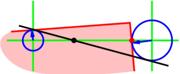
The major limitation of this simple technique is that the samples on S∗are not necessarily close to S in the vicinity of sharp features. Figure 3 shows an extreme example in two dimensions, i.e., contour extraction from a two dimensional distance field. Here the distance field interpolation fails because both grid points find their minimum distance in different directions. This directional information is not captured by the scalar valued distance samples and hence the in-terpolant f∗ is an insufficient approximation of the true distance field f . Figure 5 shows this effect in a three dimensional example.
Figure 3: Consider two neighboring grid points (green) in the vicin-ity of a sharp feature (corner) of the contour S (red). Sampling the scalar valued distance function f at both grid points (blue) and mating the sample point by linear interpolation leads to a bad esti-mation (black) of the true intersection point between the red contour and the green cell edge.
To improve the approximationkf−f∗kone could refine the dis-cretization grid h→h0<h or switch to higher order polynomial
interpolants within each cell Ci,j,k(h). However, in the first case the improved accuracy of the samples comes with a refined triangula-tion and hence a larger number of triangles in the output mesh and in the second case the local computations are getting more compli-cated which affects the overall simplicity of the algorithm.
Therefore we suggest a third alternative to avoid these difficulties by using a different discretization of the distance field f which we call the directed distance field. For this data structure we exploit the fact that the Marching Cubes algorithm computes surface samples only on the cell edges. Consequently, it is not necessary to generate a continuous function f∗ which approximates f in the interior of the cells.
For the directed distance field, we store at each grid point gi,j,k three directed distances in (positive) x, y, and z direction instead of the scalar valued distances di,j,k, i.e.,
di,j,k =
" distx
disty distz
#
Negative distance values again indicate that the grid point lies inside the object while positive distances point outside.
The processing of directed distance fields is identical to the pro-cessing of scalar distance fields. The min/max computations for the boolean operations have to be applied componentwise to the di-rected distances, e.g., the didi-rected distance field for S=S1∩S2is
obtained by
di,j,k =
" max{dist
1,x,dist2,x} max{dist1,y,dist2,y} max{dist1,z,dist2,z}
# .
The Marching Cubes algorithm can be applied to the directed dis-tance field data structure without significant modifications. The lo-cal configuration can still be derived from the sign pattern at the cell’s corners since the three directed distances at one grid point always have the same sign (inside/outside status).
The intersection point, e.g., for the cell edge between gi,j,kand
gi+1,j,kis computed by
s = (1− |di,j,k[x]|/h)gi,j,k + (|di,j,k[x]|/h)gi+1,j,k and is valid if di,j,k[x]and di+1,j,k[x]have opposite signs.
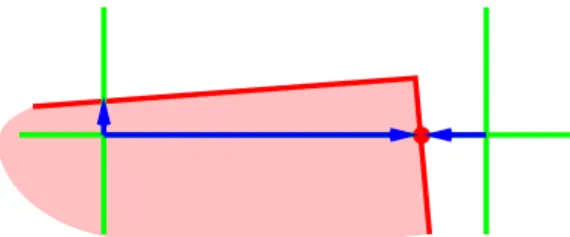
Although storing the directed distances di,j,kincreases the mem-ory consumption by a factor of three, we have the advantage that sample points lying exactly on the surface S are available for the Marching Cubes algorithm (cf. Fig. 4). As demonstrated in Fig-ure 5, this improves the quality of the extracted surface significantly in the vicinity of sharp features.
Figure 4: If we store directed distances (blue) in x and y direction at every grid point (green), we can compute exact intersection points of the contour with the cell’s edges.
3.1 Generation of directed distance fields
It appears computationally more involved to evaluate the directed distances compared to the scalar distances. However, for most types of input data it turns out that directed distances are relatively easy to compute. In fact, the average computational effort is lower than for scalar valued distance computations (where we have to search in all directions) and also lower than for general ray tracing (where
intersections can happen everywhere along the ray). We will focus on computational methods for the distance field evaluation although recently, graphics hardware accelerated techniques have been sug-gested [11].
Two different approaches are possible. One is to compute the intersections for each cell edge separately. Here we can exploit the locality of the interrogation since each edge has only a small length h. Notice that for all discrete volume representations, dis-tances with an absolute value larger than h are irrelevant since they are not used for sample point computations during the Marching Cubes algorithm.
The second approach is to combine collinear cell edges, e.g., to concatenate the grid points g0,j,k, . . . ,gn,j,kinto one axis aligned ray
g(λ) =g0,j,k+λ[1,0,0]and then compute all intersections along this ray. The intersection points are then used to store the directed distances at the corresponding grid points gi,j,k.
Implicit surfaces For a geometric object defined by an implicit function f we find the directed distances for a grid point by a
uni-variate root finding scheme [24] which becomes particularly simple
since we only search along the x, y, or z axis, e.g., for the edge be-tween the grid points gi,j,kand gi+1,j,k, we have to solve
˜
f(t) = f(i h+t,j h,k h) =0, t∈[0,1].
For a reasonably small grid size h we can find a sufficiently good starting value for t and Newton iterations will quickly converge to the exact solution. Notice that closest point search for an implicit surface is much more complicated than ray intersection [4]. Polygonal meshes If our geometric object is given by a polyg-onal mesh, the directed distance computation can use all the ac-celeration techniques that have been developed for fast ray-tracing algorithms [2]. In our implementation we use a binary space
parti-tion tree [35] to quickly find the triangles which are candidates for
an intersection. For each grid point gi,j,kwe identify the triangles in a h+εsphere and then compute intersections with the axis aligned rays in positive x, y, and z directions.
Since we know that our inquiry points gi,j,k lie on a uniform spatial grid we can exploit this regular structure to optimize the BSP-tree. In fact, using the octree space partitioning implied by the grid cells Ci,j,k(h)themselves seems to be the optimum.
Point clouds Volume representations for point clouds are an ef-fective tool which is used in many surface reconstruction algorithms [7, 17]. To define a signed distance to the point cloud, each point has to be equipped with a properly oriented normal vector [1, 17].
Together with its normal each point defines a tangent plane ele-ment and the signed distance from a query point gi,j,kto the cloud is defined as the signed distance to the tangent plane of the nearest neighbor.
Computing directed distances requires the intersection of rays with the point cloud. In our implementation we used a variation of the technique proposed in [9, 36].
4
Extended Marching Cubes
Even if we are able to compute exact surface samples with the di-rected distance field data structure, the major problem with any dis-cretization of a distance field f remains. This is the occurrence of alias effects at sharp features of the underlying surface S. In prin-ciple, we could reduce the approximation error of the surface S∗ extracted from the discretized field f∗ by excessively refining the grid cells in the vicinity of the feature. However, the normals of the extracted surface S∗ will never converge to the normals of S (cf. Fig. 6).
Figure 5: The center and right surfaces are generated by the Marching Cubes algorithm applied to the uniformly sampled distance field of the object on the left. In the center, scalar distance values are stored for each grid point while on the right three directed distances are stored to enable exact surface sampling. This reduces the alias errors to a small region around the feature.
Figure 6: Alias errors in surfaces generated by the Marching Cubes algorithm are due to the fixed sampling grid. By decreasing the grid size, the effect becomes less and less visible due to the convergence of S∗ to S but the problem is not really solved since the normal vectors of S∗do not converge to the normals of S.
The reason for this behavior is the fact that the standard March-ing Cubes algorithm computes surface samples on a globally uni-form grid that cannot be aligned to the features of the object. Lo-cally adapting the sampling grid to the features of an object is criti-cal since we do not want to lose the advantageous properties of the basic algorithm like simplicity and efficiency.
Using higher order approximants to the local surface patch in-stead of piecewise linear meshes does not improve the situation since the sharp feature of an object’s surface S are exactly the loca-tions where the surface is not a differentiable manifold.
However, what we can do is to use additional local information from the distance field f and to extrapolate the behavior of the sur-face near the feature. Figure 7 depicts the technique in two dimen-sions. Instead of directly connecting the intersection points of the contour with the cell edges, we additionally use the contour normal to compute a linear local approximation (tangent element) for each intersection point. Then intersecting the two tangents yields an ad-ditional sampling point close to the sharp feature. If we include this additional sample into our piecewise linear contour approximation we obtain a much better reconstruction. A similar technique for 2-dimensional contour curve reconstruction has been proposed in [38]. While their method is based on higher order polynomial in-terpolants to several consecutive sample points, we use higher order data from one single sample.
This effect did not happen by chance. As we stated earlier, the surface/contour near a sharp feature is not a differentiable manifold. However, for reasonable geometric models, we can at least assume that the surface is piecewise differentiable. Hence, using point and normal information to generate tangent elements yields good ap-proximations on both sides of the feature and the intersection of these approximations gives a good estimate of the actual feature position.
From approximation theory we know that a piecewise linear
in-Figure 7: By using point and normal information on both sides of the sharp feature one can find a good estimate for the feature point at the intersection of the tangent elements.
terpolant to a smooth surface converges with the order O(h2)where h measures the sampling density. In our case h is the size of the grid
cell. If we uniformly refine the grid h→h/2 we can expect the ap-proximation error the be reduced to 1/4. However, in those cells with sharp features the surface is not differentiable and hence the approximation order drops down to O(h) which means the error decreases much slower (in fact proportional to the grid size).
Using the tangent element approximation, however, increases the local convergence rate in those feature cells since the (quadratic order) approximation is done on both sides of the feature separately. Of course for this argument to be valid we have to assume that there is only one sharp feature within each cell but, again, this will be the case for reasonable models and sufficient grid refinement.
In our extended Marching Cubes algorithm we generalize this univariate feature point extrapolation technique to surfaces. How-ever, the situation is more complicated since different types of fea-tures have to be handled in a different manner. These types are
feature edges where two smooth surface regions meet along a sharp
feature line and corners where more than two smooth components meet or, equivalently, where more than two feature edges intersect. Just like the standard Marching Cubes, the extended algorithm processes each cell Ci,j,k(h)separately. For each cell we first have to check if a feature is present and if yes, which type of feature (cf. Fig. 8). This classification of the cells is similar to the classi-fication of cells in the extended octree data structure [6] where the leaves of an octree for a CSG model are tagged as face cells, edge
cells, and vertex cells respectively.
If the cell does not contain a sharp feature, we generate a local triangle mesh patch by using the standard Marching Cubes table. However, if a feature is present, we use the gradient information at the edge intersection points to define local tangent elements. Based on these planes we compute one new sample point close to the ex-pected feature. Instead of using the standard triangulation we gen-erate a triangle fan with the new vertex as its center.
Figure 8: When inserting additional feature samples in some cells during the extended Marching Cubes we distinguish between dif-ferent types of feature configurations: edge features are shown in green and corner features in red.
use the global uniform sampling grid to compute points on the sur-face S but we include additional sample points in those cells where we expect sharp features. Hence we combine the advantages of reg-ular data structures with the flexibility of adaptive sampling. Notice that for typical CAD models the feature sampling will happen only in very few cells along the feature lines.
Figure 9: The feature sensitive sampling in the extended March-ing Cubes algorithm works in three steps. First, the cells/patches that contain a feature are identified (left). Then one new sample is included per cell (center) and finally one round of edge flipping reconstructs the feature edges.
Figure 9 shows the different stages of the algorithm. Since the feature samples are inserted into the mesh as the center of a triangle fan without considering neighboring cells, the triangle connectiv-ity of the resulting mesh does not reflect the presence of features. Hence, we have to apply a postprocessing step to the mesh where some of the mesh edges are flipped. The flipping criterion is quite simple: each edge is flipped if it will connect two feature samples
after the flip. The edge flipping does not produce any undesired
side effects since the restriction to one feature sample per cell guar-antees their sufficient separation. After the flipping, the edges con-necting feature samples provide an explicit representation of the feature lines as polygons within the triangle mesh. In Figure 10 we show the results of the extended Marching Cubes algorithm for the same dataset that has been used in Figure 5.
After this general description of the algorithm, the remaining technical questions are, how to do the feature classification and how to compute the feature sample point. There are different ways to implement this functionality. The solutions that we present here are designed to not contain any unintuitive parameter and to find the optimal position for the feature sample.
4.1 Surface normals
Feature detection and sampling both need additional information about the surface S. In addition to the position of the sample points,
their normal vectors are required to construct the local tangent el-ements. We have shown in the last section how an alternative dis-cretization of the continuous distance field f yields exact point sam-ples. For the surface normal information we have to exactly evalu-ate the gradient of the distance field as well.
Since the gradient information is only needed at the sample lo-cations, we can evaluate the gradients in advance during the dis-cretization of the distance field. In our implementation we store the gradients in the same data structure.
Implicit surfaces If an analytic function f is known for the sur-face S then the gradient can be evaluated exactly at any location. For this we have to compute the derivatives with respect to all three coordinates symbolically. If the function f or its derivatives are too complicated then numerical estimates based on divided differences yield sufficiently good estimates.
Polygonal meshes During the evaluation of the (directed) dis-tance to a polygon mesh we find the closest point on the surface as a by-product. The normalized vector pointing from the query point to that closest point is the normalized gradient of the distance field. For our extended Marching Cubes algorithm we have to evaluate the gradient of the distance function only for sample points lying exactly on the surface S. Hence, we can simply use the normal vector of that triangle on which the sample point lies.
Point clouds When computing the distance to a point cloud or when intersecting a ray with it, we replace the scattered points by tangent elements which can be considered as small facets making up a polygonal surface. Hence the situation is quite similar to the distance field computations for polygonal meshes: We find the gra-dients for the surface samples by taking the normal vector associ-ated with the nearest scattered point.
Scalar distance fields In some applications it might happen that we get a discretized scalar valued distance field out of some pre-process such that we cannot access the original continuous dis-tance function f . In this case we have to estimate the gradients from the scalar distance values at the grid points.
There are two possibilities: the first is to compute the gradient of the tri-linear interpolant, the second is to estimate the gradient in each grid point by divided differences using neighboring grid points. These grid point gradients can then be interpolated within each cell.
It is not obvious which method is superior to the other. The second technique guarantees a continuous gradient field (which the first method does not) but due to the larger support of the divided difference operator we can observe a blurring effect on the gradient field which makes the detection of sharp features more difficult.
4.2 Feature detection
Let s0, . . . ,snbe surface samples obtained by intersecting the edges of an octree cell Ci,j,k(h)with the surface S defined by f(x,y,z) =0. If the constellation of the edge/surface intersection indicates (ac-cording to the standard Marching Cubes table) the occurrence of more than one connected component then we assume that the siare a subset of the edge intersection that belong to the same component. The selection of the siis done based on the Marching Cubes table. In cells with several unconnected components we apply the edge detection and feature sampling for each component separately.
Let nibe the unit surfaces normals of S at si, i.e., the normalized gradients of f . Our goal is to detect if the surface patch of S corre-sponding to the samples sicontains a sharp feature. One simple but
Figure 10: The original object on the left is converted into a volume representation with the same resolution as in Fig. 5. In the center and on the right we applied the extended Marching Cubes algorithm with feature sensitive sampling. The necessary gradient information is estimated from the discrete scalar distance field in the center and evaluated from the original distance field on the right. The result of the combination of the directed distance field with the extended Marching Cubes algorithm is indistinguishable from the original.
quite effective heuristic to do this is to compute the opening angle of the normal cone spanned by the ni. If
θ := mini,j(nTi nj)
is smaller than some thresholdθsharpthen we expect the surface
to have a sharp feature. Let n0and n1be the two normals which
enclose the largest angle and n∗=n0×n1be the normal vector to
the plane spanned by n0and n1.
Next, we have to determine if the detected feature is a sharp edge or if it is a corner point. For this we estimate the maximum devia-tion of the normals nifrom the plane spanned by n0and n1, i.e., we
compute
ϕ := maxi|nTi n∗|
and test if it is greater than some thresholdϕcorner. These simple
criteria proved to be quite effective in all applications reported in Section 5. The two parametersθsharpandϕcornerare very intuitive
since they can be considered as threshold angles that measure the sharpness of a feature. The thresholdθsharpcan be chosen quite big,
sayθsharp=0.9, if the gradient data is not too noisy. For stability
reasons in the subsequent calculations, however, it is advisable to choose the corner thresholdϕcornerbig enough, sayϕcorner=0.7,
to reduce the number of erroneous classifications. This is necessary to distinguish between sharp corners and curved feature lines. In all our experiments, the feature detection worked robustly without being too sensitive to the particular choice of the threshold parame-ters. Artifacts can only occur if edge features are wrongly classified as corners (cf. next section).
4.3 Feature sampling
Once we have the classification of the current cell Ci,j,k(h) as a feature line (θ<θsharp,ϕ≤ϕcorner) or as a corner configuration
(θ<θsharp,ϕ>ϕcorner) we try to find a sample point as close as
possible to the feature. As explained above we generate a tangent element for each sample si with its normal niand place the fea-ture sample at the intersection of all tangent elements, i.e., the new sample p solves the linear system
[. . . ,ni, . . .]Tp = [. . . ,nTi si, . . .]. (1) In general this system is overdetermined since we usually have more than three edge intersections in each cell Ci,j,k(h). However, at feature edges it can also happen that this system is underdeter-mined since at a perfect feature edge, the tangent elements[si,ni] are all sampled from two different planes and hence the matrix of normal vectors has only rank two.
To avoid the handling of special cases, we therefore solve the system (1) with the pseudo-inverse based on the singular value de-composition of N= [. . . ,ni, . . .]T [16]. If the feature is classified as corner then this is a very stable way to compute the optimal fea-ture sample point in the least squares sense, i.e. we find the point
p where the average (squared) deviation from all tangent elements
takes on its minimum.
If the feature is classified as an edge we expect one of the sin-gular values to vanish since the (straight) feature line lies in both tangent planes. However on real data this will almost never happen since the gradient samples might be affected by arithmetic noise, the surfaces near the feature might be curved, or the feature line might be curved itself. Since the angle criteria used for the classi-fication decided for a feature edge configuration, we therefore set the smallest singular value of N explicitly to zero thus enforcing the proper structure of the (now) rank deficient system (1). By this we suppress the influence of those normal vectors which strongly devi-ate from the plane spanned by n0and n1and stabilize the solution
of (1). Mis-classifying an edge feature as a corner and consequently not setting the smallest singular value to zero, can lead to bad esti-mates for p.
The pseudo-inverse of the modified matrix ˜N will lead to the
least norm solution of the underdetermined system, i.e. we find that point p on the feature line which is closest to the origin. In order to guarantee that this point lies in a reasonable configuration to the samples siwe apply a coordinate transform to the samples before setting up the system (1) such that their center of gravity lies in the origin.
Remarks We described the feature sampling procedure as a two step process. First the feature is classified by the opening angles of the normal cone. Then the tangent plane intersection in solved based on the singular value decomposition of the normal matrix N. It is tempting to try to read off the feature classification of the local configuration directly from the magnitude of the singular values. However it turns out that this is a very unreliable criterion since the singular values not only depend on the angles between the normals but also on their distribution.
If a feature edge passes through a cell Ci,j,k(h)we can have up to seven intersection points belonging to the same surface compo-nent for which we want to compute one additional feature sam-ple. A priori we do not have any information about how many of those samples lie on either side of the feature. This makes the singular value classification quite unreliable since the matrix
[n0,n0,n0,n0,n0,n1]has a very different singular value
5
Applications
In order to demonstrate the effectiveness of our new surface ex-traction scheme we will point out different applications. In princi-ple, the extended Marching Cubes can always replace the original Marching Cubes algorithm since it has the same algorithmic struc-ture and processes the same type of input data. If the distance field gradients cannot be evaluated at the sample points, they can be es-timated from the tri-linear interpolant (cf. Sect. 4.1).
Obviously the standard Marching Cubes scheme will always out-perform our extended version since we have to do more involved computations for every cell. However, the feature sampling has to be done only in those cells where a feature configuration has been detected from the normal cone and their number will increase only linearly with the refinement while the total number of cells that con-tain a piece of the surface grows quadratically. Moreover, we ob-served that the necessary refinement levels for a given accuracy is often lower with the extended Marching Cubes algorithm because the feature sampling reduces the approximation error significantly.
The following table shows the relevant parameters for the models depicted in this section. The execution times include only the running times for the standard and extended Marching Cubes, respectively. The (directed) distance fields and gradients have been generated in a pre-process. The triangle count is always higher for the extended Marching Cubes since we always chose the same refinement level for both algorithms – although the approximation error turned out to be much lower for the extended Marching Cubes.
standard MC extended MC
secs kTris secs kTris
CSG (Fig. 11) 4.03 105 5.48 117
Fan Disk (Fig. 1) 0.67 19 1.40 21
Max Planck (Fig. 14) 2.77 74 3.31 79
CAD (Fig. 15) 1.69 48 2.4 54
Figure 11: This figure shows a CSG example where the hollow letters are subtracted from a cube-shaped base object. Directed dis-tances and surface normals are derived directly from the volume representation of the individual parts. The right image shows the pieces that are generated in the interior of the cube by the three cuts.
5.1 CSG modeling
The classical application area for volume representations is the de-sign of solid objects by boolean operations. Every operation can be performed by simple comparison of the distance values at the grid points. This also holds for the directed distance field representation.
In our implementation we use the extended Marching Cubes for the mesh generation from a CSG model. Feature sensitive sampling is very important in this context since the sharp edges and corners indicate intersections of basic objects and carry significant design information (cf. Fig. 11).
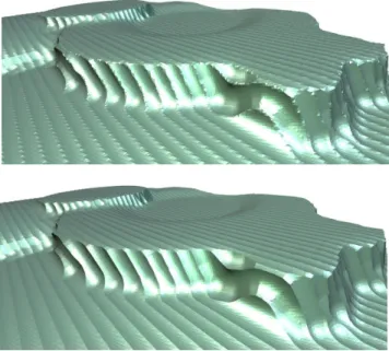
A very important practical application of this technique is the simulation of milling processes. A milling tool is traced along a path and its envelope surface has to be generated. This application is very demanding for the solid modeling tool since the envelope surface usually intersects itself many times. The sharp ridges that are characteristic for surfaces generated by a milling machine carry crucial information because they are used to rate the quality of the NC program (cf. Fig. 12).
Figure 12: Here we show the result of a milling simulation. The volume representation of the milling tool’s envelope has been gen-erated with boolean “join” operations applied to instances of the milling tool at different time steps. Since the path of the milling tool is piecewise linear, the envelope can be constructed from cylin-ders and spheres. The upper image shows the surface extracted by the standard MC algorithm, the lower image shows the extended MC surface. The sharp ridges are better visible due to the clearly reduced alias.
5.2 Surface reconstruction
One well-established technique to reconstruct a polygonal mesh model from an unstructured cloud of points is to estimate a signed distance function and then apply the Marching Cubes algorithm [7, 17]. As we showed in Section 3.1 it is also possible to com-pute directed distances and gradient information from point clouds if normal vectors are available for the scattered points. We show an example surface reconstructed from a dataset with 200K points in Fig. 13.
Since scattered point datasets often come from a 3D scanning device, they are usually disturbed by noise which affects the quality of the resulting 3D models. Many optimization techniques have been proposed to improve the smoothness of polygonal models by applying local filter operations [8, 27, 41].
For meshes that we generated with the extended Marching Cubes algorithm, we not only have the pure geometric information but we additionally have some mesh vertices tagged as feature points and some edges (connecting two feature points) classified as sharp
Figure 13: Triangle mesh reconstruction from a 3D scan of a bust. The original dataset consists of 200 K scattered points. On the left we show the result by the standard MC and on the right the extended marching cubes. The right model is less blurred and shows much more details around the mouth.
feature edges. We can exploit this information to further improve the surface quality in the smoothing step by applying a univariate smoothing scheme to the feature lines and a bivariate smoothing scheme to the non-feature areas. If we disallow tangent information to propagate across feature lines we can even enhance the sharpness of the features. Figure 14 shows an example.
Figure 14: The left image show the result of the extended MC ap-plied to a point cloud. If we low pass filter the mesh by taking the feature information into account we obtain the result on the right. All sharp features are well preserved while in the non-feature areas, noise is effectively removed.
5.3 Remeshing
Polygonal meshes that are generated at some intermediate stage of an industrial CAD process often have a bad quality. Degenerate tri-angles and topological inconsistencies make it difficult to use such models in any downstream application. To make this data accessi-ble to other applications than mere display, we have to convert the models into enhanced tesselations of the same geometry that guar-antee, e.g., bounds on the aspect ratio of the triangular faces. This resampling procedure is usually called remeshing [10, 29].
We converted a CAD model into a volume representation by sampling its distance field on a uniform grid. Applying the ex-tended Marching Cubes algorithm to this volume gives a remeshed version of the original with a uniform vertex distribution.
One apparent drawback of Marching Cubes techniques in gen-eral is the uniform sampling density which does not take the local
Figure 15: Remeshing of a polygonal mesh. The upper mesh has been generated from a CAD model and has a very bad distribution of triangles. We sampled the distance field for the model on a[129]3
grid and reconstructed the surface by the standard MC algorithm (second image). The actual resolution of the volume representation can be see from the sizes of the artifacts in the reconstructed sur-face. In the third image we show our extended MC result. All sharp features are reconstructed correctly (θsharp=0.9). The lower
im-age shows the result of a feature line preserving mesh decimation algorithm (error tolerance 1%).
surface curvature into account. Many approaches have been pro-posed to control the mesh complexity by adaptive octree descent with sophisticated refinement criteria [20, 37].
Similar to the feature sensitive smoothing we can exploit the fea-ture information in the extended Marching Cubes output to control the behavior of a mesh decimation post-process. In our implemen-tation we use a mesh decimation scheme that is based on edge col-lapsing [14, 19, 28]. Feature vertices are not allowed to change their position during an edge collapse unless the collapsed edge is a feature edge. By this we obtain effectively decimated meshes that preserve most of the relevant feature information (cf. Fig. 15).
6
Conclusions and future directions
We presented a new mesh generation technique which converts a distance field representation of a geometric model into a polygo-nal mesh representation. Based on the Marching Cubes paradigm we derived an extended algorithm that is able to reliably detect and classify sharp feature regions on the surface and to accurately sam-ple these features in order to reduce alias artifacts.
For the standard Marching Cubes there are generalizations that can be applied to adaptively refined balanced octrees [20, 37]. The problem here is to fix the gaps that appear in areas where cells from different refinement levels meet. We are planning to modify the extended Marching Cubes such that balanced octrees can be pro-cessed as well. Currently, we do use adaptively refined octrees but our refinement criterion always guarantees that the “crust” contain-ing the actual surface is refined down to the finest level.
Finally, we did not optimize our extended Marching Cubes code for computation speed. In principle there would be plenty of room for improvements in various algorithmic steps of our current im-plementation. However, we are aiming at a parallelization of the algorithm. Crucial difficulties are not to be expected since the algo-rithm processes each cell individually (like the standard Marching Cubes) and hence parallelization should be straightforward.
References
[1] N. Amenta, M. Bern, M. Kamvysselis, A New Voronoi-Based Surface
Recon-struction Algorithm, Computer Graphics (SIGGRAPH 98 Proceedings), 1998,
415 – 422
[2] J. Arvo, D. Kirk, A Survey of Ray Tracing Acceleration Techniques, An Intro-duction to Ray Tracing (A. Glassner, ed.), Academic Press, 1989, 201 – 262
[3] J. Bloomental, Polygonization of implicit surfaces, CAGD 5, 1988, 341 – 355
[4] J. Bloomental, C. Bajaj, J. Blinn, M. Cani-Gascuel, A. Rockwood, B. Wyvill, G. Wyvill, Introduction to implicit surfaces, Morgan Kaufmann Publishers, 1997
[5] D. Breen, S.Mauch, R. Whitaker, 3D scan conversion of CSG models into
dis-tance volumes, IEEE Symposium on Volume Visualization, 1998, 7 – 14
[6] P. Brunet, I. Navazo, Solid representation and operation using extended octrees, ACM Trans. on Graphics 9 (1990) 2, 170 – 197
[7] B. Curless, M. Levoy, A Volumetric Method for Building Complex Models from
Range Images, Computer Graphics (SIGGRAPH 96 Proceedings), 1996, 303 –
312
[8] M. Desbrun, M. Meyer, P. Schröder, A. H. Barr, Implicit Fairing of Irregular
Meshes Using Diffusion and Curvature Flow, Computer Graphics (SIGGRAPH
99 Proceedings), 1999, 317 – 324
[9] P. Dutre, P. Tole, D. Greenberg, Approximate visibility for illumination
com-putations using point clouds, Technical report PCG-00-1, Cornell University,
2000
[10] M. Eck, T. DeRose, T. Duchamp, H. Hoppe, M. Lounsbery, W. Stuetzle,
Mul-tiresolution Analysis of Arbitrary Meshes, Computer Graphics (SIGGRAPH 95
Proceedings), 1995, 173 – 182
[11] K. Hoff, T. Culver, J. Keyser, M. Lin, D, Manocha, Fast computation of
gen-eralized Voronoi diagrams using graphics hardware, Computer Graphics
(SIG-GRAPH 99 Proceedings, 1999, 277 – 286
[12] J. Foley, A. van Dam, S. Feiner, J. Hughes, Computer Graphics: Principles and
Practice, Addison–Wesley, 1992
[13] S. Frisken, R. Perry, A. Rockwood, T. Jones, Adaptively sampled distance
fields: a general representation of shape for computer graphics, Computer
Graphics (SIGGRAPH 00 Proceedings), 2000, 249 – 254
[14] M. Garland, P. S. Heckbert, Surface Simplification Using Quadric Error
Met-rics, Computer Graphics (SIGGRAPH 97 Proceedings), 1997, 209 – 218
[15] S. Gibson, Using Distance Maps for Accurate Surface Representation in
Sam-pled Volumes, IEEE Symposium on Volume Visualization, 1998, 23 – 30
[16] G. Golub, C. van Loan, Matrix Computations, 3rd, Johns Hopkins Univ Press, 1996
[17] H. Hoppe, T. DeRose, T. Duchamp, J. McDonald, W. Stuetzle, Surface
Recon-struction from Unorganized Points, Computer Graphics (SIGGRAPH 92
Pro-ceedings), 1992, 71 – 78
[18] H. Hoppe, T. DeRose, T. Duchamp, M. Halstead, H. Jin, J. McDonald, J. Schweitzer, W. Stuetzle, Piecewise smooth surface reconstruction, Computer Graphics (SIGGRAPH 1994 Proceedings), 1994, 295 – 302
[19] H. Hoppe, Progressive Meshes, Computer Graphics (SIGGRAPH 96 Proceed-ings), 1996, 99 – 108
[20] Y. Livnat, H. Shen, C. Johnson, A near optimal isosurface extraction algorithm
using span space, IEEE Trans. Visualization and Computer Graphics, 1996
[21] W. Lorensen, H. Cline, Marching Cubes: a high resolution 3D surface
con-struction algorithm, Computer Graphics (SIGGRAPH 87 Proceedings), 1987,
163 – 169
[22] J. Huang, R. Yagel,V. Filippov, Y. Kurzion, An Accurate Method for Voxelizing
Polygon Meshes, ACM 1998 Symposium on Volume Visualization, 1998, 119
– 126
[23] M. Kass, A.Witkin, D. Terzopoulus, Snakes: Active Contour Models, Interna-tional Journal of Computer Vision, 1988, 321 – 331
[24] D. Kalra, A. Barr, Guaranteed ray intersections with implicit surfaces, Com-puter Graphics (SIGGRAPH 89 Proceedings), 1989, 297 – 306
[25] A. Kaufman, Efficient Algorithms for 3D Scan–Conversion of Parametric
Curves, Surfaces, and Volumes, Computer Graphics, 21, 4, 1987, 171 – 179
[26] A. Kaufman, D. Cohen, R. Yagel, Volume Graphics, IEEE Computer, Vol. 26, No. 7, July 1993, 51 – 64
[27] L. Kobbelt, S. Campagna, J. Vorsatz, H-P. Seidel, Interactive Multi-Resolution
Modeling on Arbitrary Meshes, Computer Graphics (SIGGRAPH ’98
Proceed-ings), 1998, 105 – 114
[28] L. Kobbelt, S. Campagna, H-P. Seidel, A general framework for mesh
decima-tion, Graphics Interface ’98 Proceedings, 1998, 43 – 50
[29] A. Lee, W. Sweldens, P. Schröder, L. Cowsar, D. Dobkin, Multiresolution
adap-tive parameterization of surfaces, Computer Graphics (SIGGRAPH 98
Pro-ceedings), 1998, 95 – 104
[30] C. Lürig, L. Kobbelt, T. Ertl, Deformable surfaces for feature based indirect
vol-ume rendering, Computer Graphics International, IEEE Proceedings, 1998,752
– 760
[31] C. Montani, R. Scateni, R. Scopigno, Discretized marching cubes, IEEE Visu-alization Conference Proceedings, 1994, 281 – 287
[32] C. Montani, R. Scateni, R. Scopigno, A modified look-up table for implicit
dis-ambiguation of Marching Cubes, The Visual Computer (10), 1994, 353 – 355
[33] G. Nielson, B. Hamann, The asymptotic decider: resolving the ambiguity in
marching cubes, Visualization ’91, IEEE Computer Society Press, 1991, 83 –
91
[34] A. Rappoport, S. Spitz, Interactive boolean operations for conceptual design of
3D solids, Computer Graphics (SIGGRAPH 97 Proceedings), 1997, 269 – 278
[35] H. Samet, The Design and Analysis of Spatial Data Structures, Addison– Wesley, 1989
[36] G. Schaufler, H. Wann Jensen, Ray tracing point sampled geometry, Eurograph-ics Rendering Workshop Proceedings, 2000, 319 – 328
[37] R. Shekhar, E. Fayyad, R. Yagel, J. Cornhill, Octree-based Decimation of
Marching Cubes Surfaces, Visualization ’96, IEEE Conference Proceedings,
1996, 335 – 342
[38] K. Siddiqi, B. Kimia, C. Shu, Geometric Shock-Capturing ENO Schemes for
Subpixel Interpolation, Computation and Curve Evolution, Graphical models
and image processing (59), 1997, 278 – 301
[39] B. Stander, J. Hart, Guaranteeing the topology of an implicit surface
polygo-nization for interactive modeling, Computer Graphics (SIGGRAPH 97
Pro-ceedings), 1997, 279 – 286
[40] D. Terzopoulus, Regularization of Inverse Visual Problems Involving
Disconti-nuities, IEEE Transactions on Pattern Analysis and Machine Intelligence, 1986
[41] G. Taubin, A Signal Processing Approach to Fair Surface Design, Computer Graphics (SIGGRAPH 95 Proceedings), 1995, 351 – 358
[42] G. Turk, J. O’Brien, Shape transformation using variational implicit functions, Computer Graphics (SIGGRAPH 99 Proceedings), 1999, 335 – 342 [43] Z. Wood, M. Desbrun, P. Schröder, D. Breen, Semi-Regular Mesh Extraction