Clarida, Galí, Gertler: The Science of Monetary Policy
The Science of Monetary Policy:
A New Keynesian Perspective
Richard Clarida, Jordi Galí,
and
Mark Gertler
1 “Having looked at monetary policy from both sides now, I can testify that central banking in practice is as much art as science. Nonetheless, whilepracticing this dark art, I have always found the science quite useful.”2
Alan S. Blinder
1. Introduction
T
HERE HAS BEEN a great resurgence of interest in the issue of how to con-duct monetary policy. One symptom of this phenomenon is the enormous vol-ume of recent working papers and con-ferences on the topic. Another is that over the past several years many leading macroeconomists have either proposed specific policy rules or have at least staked out a position on what the general course of monetary policy should be. John Taylor’s recommendation of a sim-ple interest rate rule (Taylor 1993a) is a well-known example. So too is the recent widespread endorsement of inflation tar-geting (e.g., Ben Bernanke and Frederic Mishkin 1997).Two main factors underlie this re-birth of interest. First, after a long pe-riod of near exclusive focus on the role of nonmonetary factors in the business cycle, a stream of empirical work begin-ning in the late 1980s has made the case that monetary policy significantly influ-ences the short-term course of the real economy.3 The precise amount remains open to debate. On the other hand, there now seems to be broad agreement that the choice of how to conduct monetary policy has important conse-quences for aggregate activity. It is no longer an issue to downplay.
Second, there has been considerable improvement in the underlying theoret-ical frameworks used for policy analysis. To provide theoretical underpinnings, the literature has incorporated the tech-niques of dynamic general equilibrium theory pioneered in real business cycle
1661
1 Clarida: Columbia University and NBER; Galí:
New York University, Universitat Pompeu Fabra, CEPR, and NBER; Gertler: New York University and NBER. Thanks to Ben Bernanke, Bob King, Ben McCallum, Albert Marcet, Rick Mishkin, Athanasios Orphanides, Glenn Rudebusch, Chris Sims, Lars Svensson, Andres Velasco, and several anonymous referees for helpful comments, and to Tommaso Monacelli for excellent research assis-tance. Authors Galí and Gertler are grateful to the C.V. Starr Center for Applied Economics, and (Galí) to CREI for financial support. e-mail: mark.gertler@econ.nyu.edu
2 Blinder 1997, p. 17.
3 Examples include Romer and Romer (1988),
Bernanke and Blinder (1992), Galí (1992), Ber-nanke and Mihov (1997a), Christiano, Eichen-baum, and Evans (1996, 1998) and Leeper, Sims and Zha (1996). Much of the literature has fo-cused on the effects of monetary policy shocks. Bernanke, Gertler, and Watson (1997) present evi-dence that suggests that the monetary policy rule may have important effects on real activity.
analysis. A key point of departure from real business cycle theory (as we later make clear) is the explicit incorporation of frictions such as nominal price rigidi-ties that are needed to make the frame-work suitable for evaluation of monetary policy.
This paper summarizes what we have learned from this recent research on monetary policy. We review the prog-ress that has been made and also iden-tify the central questions that remain. To organize the discussion, we exposit the monetary policy design problem in a simple theoretical model. We start with a stripped-down baseline model in or-der to characterize a number of broad principles that underlie optimal policy management. We then consider the im-plications of adding various real world complications. Finally, we assess how the predictions from theory square with policy-making in practice.
Throughout, we concentrate on ex-positing results that are robust across a wide variety of macroeconomic frame-works. As Ben McCallum (1997b) em-phasizes, the key stumbling block for policy formation is limited knowledge of the way the macroeconomy works. Results that are highly model-specific are of limited use. This literature, how-ever, contains a number of useful prin-ciples about optimal policy that are rea-sonably general in applicability. In this respect there is a “science of monetary policy,” as Alan Blinder suggests in the quote above. We provide support for this contention in the pages that follow.
At the same time, we should make clear that the approach we take is based on the idea that temporary nominal price rigidities provide the key friction that gives rise to nonneutral effects of monetary policy. The propositions we derive are broadly applicable within this class of models. This approach has widespread support in both theoretical
and applied work, as we discuss later.4 There are, however, important strands of the literature that either reject the idea of nominal price rigidities (e.g., real business cycle theory) or focus on other types of nominal rigidities, such as frictions in money demand.5 For this reason, we append “New Keynesian Perspective” to the title. In particular, we wish to make clear that we adopt the Keynesian approach of stressing nomi-nal price rigidities, but at the same time base our analysis on frameworks that in-corporate the recent methodological ad-vances in macroeconomic modeling (hence the term “New”).
Section 2 lays out the formal policy problem. We describe the baseline theoretical model and the objectives of policy. Because we are interested in characterizing policy rules in terms of primitive factors, the model we use evolves from first principles. Though it is quite simple, it nonetheless contains the main ingredients of descriptively richer frameworks that are used for pol-icy analysis. Within the model, as in practice (we argue), the instrument of monetary policy is a short-term interest rate. The policy design problem then is to characterize how the interest rate should adjust to the current state of the economy.
An important complication is that pri-vate sector behavior depends on the ex-pected course of monetary policy, as well as on current policy. The credibil-ity of monetary policy thus becomes relevant, as a considerable contemporary literature has emphasized.6 At issue is
4 See, for example, the survey by Goodfriend
and King (1997).
5 See, for example, Christiano, Eichenbaum,
and Evans (1997). For an analysis of monetary pol-icy rules in these kinds of models—known as “lim-ited participation” frameworks—see Christiano and Gust (1999).
6 For a recent survey of the credibility
whether there may be gains from en-hancing credibility either by formal commitment to a policy rule or by intro-ducing some kind of institutional ar-rangement that achieves roughly the same end. We address the issue by ex-amining optimal policy for both cases: with and without commitment. Along with expositing traditional results, we also exposit some new results regarding the gains from commitment.
Section 3 derives the optimal policy rule in the absence of commitment. If for no other reason, this case is of inter-est because it captures reality: No ma-jor central bank makes any type of bind-ing commitment over the future course of its monetary policy. A number of broad implications emerge from this baseline case. Among these: The opti-mal policy embeds inflation targeting in the sense that it calls for gradual adjust-ment to the optimal inflation rate. The implication for the policy rule is that the central bank should adjust the nominal short rate more than one-for-one with expected future inflation. That is, it should adjust the nominal rate suf-ficiently to alter the real rate (and thus aggregate demand) in the direction that is offsetting to any movement in ex-pected inflation. Finally, how the cen-tral bank should adjust the interest rate in response to output disturbances de-pends critically on the nature of the dis-turbances: It should offset demand shocks but accommodate supply shocks, as we discuss.
Section 4 turns to the case with com-mitment. Much of the literature has emphasized that an inefficiently high steady state inflation rate may arise in the absence of commitment, if the cen-tral bank’s target for real output ex-ceeds the market clearing level.7 The
gain from commitment then is to elimi-nate this inflationary bias. How realistic it is to presume that a perceptive cen-tral bank will try to inadvisedly reap short-term gains from pushing output above its natural level is a matter of re-cent controversy (e.g., Blinder 1997; McCallum 1997a). We demonstrate, however, that there may be gains from commitment simply if current price set-ting depends on expectations of the fu-ture. In this instance, a credible com-mitment to fight inflation in the future can improve the current output/infla-tion trade-off that a central bank faces. Specifically, it can reduce the effective cost in terms of current output loss that is required to lower current inflation. This result, we believe, is new in the literature.
In practice, however, a binding com-mitment to a rule may not be feasible simply because not enough is known about the structure of the economy or the disturbances that buffet it. Under certain circumstances, however, a pol-icy rule that yields welfare gains rela-tive to the optimum under discretion may be well approximated by an opti-mal policy under discretion that is ob-tained by assigning a higher relative cost to inflation than the true social cost. A way to pursue this policy opera-tionally is simply to appoint a central bank chair with a greater distaste for infla-tion than society as a whole, as Kenneth Rogoff (1985) originally emphasized.
Section 5 considers a number of prac-tical problems that complicate policy-making. These include: imperfect infor-mation and lags, model uncertainty and non-smooth preferences over inflation and output. A number of pragmatic is-sues emerge, such as: whether and how to make use of intermediate targets, the choice of a monetary policy instrument, and why central banks appear to smooth interest rate changes. Among other
7 The potential inflationary bias under
discre-tion was originally emphasized by Kydland and Prescott (1977) and Barro and Gordon (1983).
things, the analysis makes clear why modern central banks (especially the Federal Reserve Board) have greatly downgraded the role of monetary aggre-gates in the implementation of policy. The section also shows how the recently advocated “opportunistic” approach to fighting inflation may emerge under a non-smooth policy objective function. The opportunistic approach boils down to trying to keep inflation from rising but allowing it to ratchet down in the event of favorable supply shocks.
As we illustrate throughout, the opti-mal policy depends on the degree of persistence in both inflation and out-put. The degree of inflation persistence is critical since this factor governs the output/inflation trade-off that the pol-icy-maker faces. In our baseline model, persistence in inflation and output is due entirely to serially correlated ex-ogenous shocks. In section 6 we con-sider a hybrid model that allows for en-dogenous persistence in both inflation and output. The model nests as special cases our forward-looking baseline model and, also, a more traditional backward-looking Keynesian frame-work, similar to the one used by Lars Svensson (1997a) and others.
Section 7 moves from theory to prac-tice by considering a number of pro-posed simple rules for monetary policy, including the Taylor rule, and a forward-looking variant considered by Clarida, Galí, and Gertler (1998; forthcoming). Attention has centered around simple rules because of the need for robust-ness. A policy rule is robust if it pro-duces desirable results in a variety of competing macroeconomic frameworks. This is tantamount to having the rule satisfy the criteria for good policy man-agement that sections 2 through 6 es-tablish. Further, U.S. monetary policy may be judged according to this same met-ric. In particular, the evidence suggests
that U.S. monetary policy in the fifteen years or so prior to Paul Volcker did not always follow the principles we have de-scribed. Simply put, interest rate man-agement during this era tended to ac-commodate inflation. Under Volcker and Greenspan, however, U.S. mone-tary policy adopted the kind of implicit inflation targeting that we argue is consistent with good policy management.
The section also considers some pol-icy proposals that focus on target vari-ables, including introducing formal inflation or price-level targets and nominal GDP targeting. There is in ad-dition a brief discussion of the issue of whether indeterminacy may cause prac-tical problems for the implementation of simple interest rate rules. Finally, there are concluding remarks in section 8.
2. A Baseline Framework for Analysis of Monetary Policy
This section characterizes the formal monetary policy design problem. It first presents a simple baseline macro-economic framework, and then de-scribes the policy objective function. The issue of credibility is taken up next. In this regard, we describe the distinc-tion between optimal policies with and without credible commitment—what the literature refers to as the cases of “rules versus discretion.”
2.1 A Simple Macroeconomic Framework
Our baseline framework is a dynamic general equilibrium model with money and temporary nominal price rigidities. In recent years this paradigm has be-come widely used for theoretical analy-sis of monetary policy.8 It has much of the empirical appeal of the traditional
8 See, e.g, Goodfriend and King (1997),
McCal-lum and Nelson (1997), Walsh (1998), and the ref-erences therein.
IS/LM model, yet is grounded in dy-namic general equilibrium theory, in keeping with the methodological ad-vances in modern macroeconomics.
Within the model, monetary policy affects the real economy in the short run, much as in the traditional Keynes-ian IS/LM framework. A key difference, however, is that the aggregate behav-ioral equations evolve explicitly from optimization by households and firms. One important implication is that cur-rent economic behavior depends criti-cally on expectations of the future course of monetary policy, as well as on current policy. In addition, the model accommodates differing views about how the macroeconomy behaves. In the limiting case of perfect price flexibility, for example, the cyclical dynamics re-semble those of a real business cycle model, with monetary policy affecting only nominal variables.
Rather than work through the details of the derivation, which are readily available elsewhere, we instead directly introduce the key aggregate relation-ships.9 For convenience, we abstract from investment and capital accumula-tion. This abstraction, however, does not affect any qualitative conclusions, as we discuss. The model is as follows:
Let yt and zt be the stochastic
compo-nents of output and the natural level of output, respectively, both in logs.10 The latter is the level of output that would arise if wages and prices were perfectly flexible. The difference between actual and potential output is an important vari-able in the model. It is thus convenient to define the “output gap” xt:
xt≡yt−zt
In addition, let πt be the period t infla-tion rate, defined as the percent change in the price level from t–1 to t; and let it
be the nominal interest rate. Each vari-able is similarly expressed as a deviation from its long-run level.
It is then possible to represent the baseline model in terms of two equa-tions: an “IS” curve that relates the out-put gap inversely to the real interest rate; and a Phillips curve that relates inflation positively to the output gap.
xt= −ϕ[it−Etπt+ 1] +Etxt+ 1+gt (2.1)
πt=λxt+βEtπt+ 1+ut (2.2) where gt and ut are disturbances terms that obey, respectively:
gt=µgt− 1+^gt (2.3)
ut=ρut− 1+^ut (2.4) where 0 ≤µ,ρ≤ 1 and where both ^gt and
u
^t are i.i.d. random variables with zero mean
and variances σg2 and σu2, respectively. Equation (2.1) is obtained by log-linearizing the consumption euler equa-tion that arises from the household’s optimal saving decision, after imposing the equilibrium condition that con-sumption equals output minus govern-ment spending.11 The resulting expres-sion differs from the traditional IS curve mainly because current output depends on expected future output as well as the interest rate. Higher ex-pected future output raises current out-put: Because individuals prefer to
9 See, for example, Yun (1996), Kimball (1995),
King and Wolman (1995), Woodford (1996), and Bernanke, Gertler, and Gilchrist (1998) for step-by-step derivations.
10 By stochastic component, we mean the
devia-tion from a deterministic long-run trend.
11 Using the market clearing condition Yt = Ct + Et,
where Et is government consumption, we can
re-write the log-linearized consumption Euler equa-tion as:
yt − et = − ϕ[it − Etπt+ 1] + Et{yt+ 1 − et+ 1}
where et≡ − log(1 −
Et
Yt)
is taken to evolve ex-ogenously. Using xt ≡ yt − zt, it is then possible to
derive the demand for output as
xt= −ϕ[it−Etπt+ 1] +Etxt+ 1+gt
smooth consumption, expectation of higher consumption next period (associ-ated with higher expected output) leads them to want to consume more today, which raises current output demand. The negative effect of the real rate on current output, in turn, reflects in-tertemporal substitution of consump-tion. In this respect, the interest elastic-ity in the IS curve, ϕ, corresponds to the intertemporal elasticity of substitu-tion. The disturbance gt is a function of
expected changes in government pur-chases relative to expected changes in potential output (see footnote 11). Since gt shifts the IS curve, it is
inter-pretable as a demand shock. Finally, add-ing investment and capital to the model changes the details of equation (2.1). But it does not change the fundamental qualitative aspects: output demand still depends inversely on the real rate and positively on expected future output.
It is instructive to iterate equation (2.1) forward to obtain
xt=Et
∑
i= 0∞
{ −ϕ[it+i−πt+ 1 +i] +gt+i} (2.5) Equation (2.5) makes transparent the degree to which beliefs about the future affect current aggregate activity within this framework. The output gap de-pends not only on the current real rate and the demand shock, but also on the expected future paths of these two variables. To the extent monetary policy has leverage over the short-term real rate due to nominal rigidities, equation (2.5) suggests that expected as well as current policy actions affect aggregate demand.
The Phillips curve, (2.2), evolves from staggered nominal price setting, in the spirit of Stanley Fischer (1977) and
John Taylor (1980).12 A key difference is that the individual firm price-setting decision, which provides the basis for the aggregate relation, is derived from an explicit optimization problem. The starting point is an environment with monopolistically competitive firms: When it has the opportunity, each firm chooses its nominal price to maximize profits subject to constraints on the frequency of future price adjustments.
Under the standard scenario, each pe-riod the fraction 1/X of firms set prices for X > 1 periods. In general, however, aggregating the decision rules of firms that are setting prices on a staggered basis is cumbersome. For this reason, underlying the specific derivation of equation (2.2) is an assumption due to Guillermo Calvo (1983) that greatly simplifies the problem: In any given pe-riod a firm has a fixed probability θ it must keep its price fixed during that pe-riod and, hence a probability 1 – θ that it may adjust.13 This probability, fur-ther, is independent of the time that has elapsed since the last time the firm changed price. Accordingly, the average time over which a price is fixed is 1 1−θ. Thus, for example, if θ = .75, prices are fixed on average for a year. The Calvo formulation thus captures the spirit of staggered setting, but facilitates the ag-gregation by making the timing of a firm’s price adjustment independent of its history.
Equation (2.2) is simply a loglinear approximation about the steady state of the aggregation of the individual firm pricing decisions. Since the equation re-lates the inflation rate to the output gap and expected inflation, it has the flavor of a traditional expectations-augmented Phillips curve (see, e.g., Olivier Blanchard
12 See Galí and Gertler (1998) and Sbordone
(1998) for some empirical support for this kind of Phillips curve relation.
13 The Calvo formulation has become quite
common in the literature. Work by Yun (1996), King and Wolman (1995), Woodford (1996) and others has initiated the revival.
1997). A key difference with the stan-dard Phillips curve is that expected fu-ture inflation, Etπt+ 1, enters additively,
as opposed to expected current infla-tion, Et− 1πt.14 The implications of this distinction are critical: To see, iterate (2.2) forward to obtain
πt=Et
∑
i= 0∞
βi[λxt+i+ut+i] (2.6) In contrast to the traditional Phillips curve, there is no arbitrary inertia or lagged dependence in inflation. Rather, inflation depends entirely on current and expected future economic condi-tions. Roughly speaking, firms set nomi-nal price based on the expectations of future marginal costs. The variable xt+i captures movements in marginal costs associated with variation in excess de-mand. The shock ut+i, which we refer to as “cost push,” captures anything else that might affect expected marginal costs.15
We allow for the cost push shock to en-able the model to generate variation in inflation that arises independently of movement in excess demand, as appears present in the data (see, e.g., Fuhrer and Moore 1995).
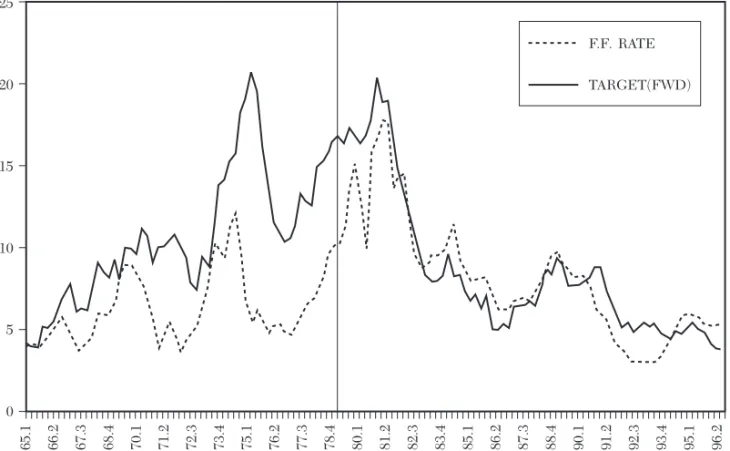
To close the model, we take the nominal interest rate as the instrument of monetary policy, as opposed to a money supply aggregate. As Bernanke and Ilian Mihov (1998) show, this as-sumption provides a reasonable descrip-tion of Federal Reserve operating pro-cedures since 1965, except for the brief period of non-borrowed reserves target-ing (1980–82) under Paul Volcker.16 With the nominal rate as the policy in-strument, it is not necessary to specify a money market equilibrium condition (i.e., an LM curve).17 In section 5, we discuss the implications of using instead a narrow monetary aggregate as the policy instrument.
Though simple, the model has the same qualitative core features as more
14 Another key difference is that the explicit
derivation restricts the coefficient λ on the output gap. In particular, λ is decreasing in θ, which mea-sures the degree of price rigidity. Thus, the longer prices are fixed on average, the less sensitive is inflation to movements in the output gap.
15 The relation for inflation that evolves from
the Calvo model takes the form πt = βEt{πt+ 1} + δ mct
where mct denotes the deviation of (real) marginal
cost from its steady state value. To then relate in-flation to the output gap, the literature typically makes assumptions on technology, preferences, and the structure of labor markets to justify a pro-portionate relation between real marginal cost and the output gap, so that mct= κxt holds, where κ is
the output elasticity of real marginal cost. In this instance, one can rewrite the relation for inflation in terms of the output gap, as follows:
πt=βEt{πt+ 1} +λxt (see Galí and Gertler (1998)
for details). In this context, the disturbance ut in
(2.2) is interpretable as reflecting deviations from the condition mct = κ xt. (Indeed the evidence in
Galí and Gertler 1998 suggests that mct does not
vary proportionately with xt). Deviations from this
proportionality condition could be caused, for ex-ample, by movements in nominal wages that push real wages away from their “equilibrium” values due to frictions in the wage contracting process.
On this latter point, see Erceg, Henderson, and Levin (1998). Another interpretation of the ut shock (suggested by Mike Woodford) is that it could re-flect a shock to the gap between the natural and potential levels of output (e.g., a markup shock).
16 Roughly speaking, Bernanke and Mihov
(1998) present formal evidence showing that the Federal Reserve intervenes in the market for non-borrowed bank reserves to support its choice for the level of the Federal Funds rate, the overnight market for bank reserves. (Christiano, Eichen-baum, and Evans 1998, though, take issue with the identifying assumptions in the Bernanke-Mihov test). Informally, Federal Reserve policy actions in recent years routinely take the form of announcing a target for the Federal funds rate (see, e.g, Rude-busch 1995). Policy discussions, further, focus on whether to adjust that target, and by how much. In this context, the view that the Funds rate is the policy instrument is widely held by both practitio-ners of monetary policy and academic researchers (see, e.g., Goodfriend 1991, Taylor 1993, and Walsh 1998).
17 With the interest rate as the policy
instru-ment, the central bank adjusts the money supply to hit the interest rate target. In this instance, the condition that money demand equal money supply simply determines the value of the money supply that meets this criteria.
complex, empirically based frameworks that are used for policy analysis.18 As in these applied frameworks, temporary nominal price rigidities play a critical role. With nominal rigidities present, by varying the nominal rate, monetary pol-icy can effectively change the short-term real rate. Through this classic mechanism it gains leverage over the near term course of the real economy. In contrast to the traditional mecha-nism, though, beliefs about how the central bank will set the interest rate in the future also matter, since both households and firms are forward look-ing. In this kind of environment, how monetary policy should respond in the short run to disturbances that buffet the economy is a nontrivial decision. Re-solving this issue is the essence of the contemporary debate over monetary policy.
2.2 The Policy Objective
The central bank objective function translates the behavior of the target variables into a welfare measure to guide the policy choice. We assume, following much of the literature, that this objective function is over the tar-get variables xt and πt, and takes the
form:
max − 1 2Et
i
∑
= 0∞ βi[αx
t+i
2 +π
t+i 2 ]
(2.7) where the parameter α is the relative weight on output deviations. Since
xt≡yt−zt, the loss function takes poten-tial output zt as the target. It also
implic-itly takes zero as the target inflation, but there is no cost in terms of generality
since inflation is expressed as a percent deviation from trend.19
While there has been considerable progress in motivating behavioral mac-roeconomic models from first princi-ples, until very recently, the same has not been true about rationalizing the objectives of policy. Over the past sev-eral years, there have been a number of attempts to be completely coherent in formulating the policy problem by taking as the welfare criterion the util-ity of a representative agent within the model.20
One limitation of this approach, how-ever, is that the models that are cur-rently available do not seem to capture what many would argue is a major cost of inflation, the uncertainty that its vari-ability generates for lifetime financial planning and for business planning (see, e.g., Brad DeLong 1997).21 Another is-sue is that, while the widely used repre-sentative agent approach may be a rea-sonable way to motivate behavioral relationships, it could be highly mis-leading as a guide to welfare analysis. If some groups suffer more in recessions than others (e.g. steel workers versus professors) and there are incomplete in-surance and credit markets, then the utility of a hypothetical representative agent might not provide an accurate barometer of cyclical fluctuations in welfare.
With certain exceptions, much of the
18 Some prominent examples include the
re-cently renovated large scale model used by the Federal Reserve Board, the FRB-US model (see Brayton, Levin, Tyron, and Williams 1997), and the medium scale models of Taylor (1979, 1993b) and Fuhrer and Moore (1995a,b).
19 Put differently, under the optimal policy, the
target inflation rate pins down the trend inflation rate. The loss function thus penalizes deviations from this trend.
20 Some examples of this approach include
Aiya-gari and Braun (1997), King and Wolman (1995), Ireland (1996a), Carlstrom and Fuerst (1995), and Rotemberg and Woodford (1997).
21 Underlying this kind of cost is the observation
that contracts are typically written in nominal terms and, for reasons that are difficult to explain, not perfectly indexed to the price level. On this issue, see the discussion in Shiller (1997) and the associated comment by Hall (1997).
literature takes a pragmatic approach to this issue by simply assuming that the objective of monetary policy is to mini-mize the squared deviations of output and inflation from their respective tar-get levels. However, Julio Rotemberg and Michael Woodford (1999) and Woodford (1998) provide a formal justi-fication for this approach. These authors show that an objective function looking something like equation (2.7) may be obtained as a quadratic approxi-mation of the utility-based welfare function. In this instance, the relative weight, α, is a function of the primitive parameters of the model.
In what follows, we simply adopt the quadratic objective given by (2.7), ap-pealing loosely to the justification of-fered in Rotemberg and Woodford (1999). Judging by the number of pa-pers written by Federal Reserve econo-mists that follow this lead, this formula-tion does not seem out of sync with the way monetary policy operates in prac-tice (at least implicitly).22 The target level of output is typically taken to be the natural level of output, based on the idea that this is the level of output that would obtain absent any wage and price frictions. Yet, if distortions exist in the economy (e.g., imperfect competition or taxes), a case can be made that the welfare maximizing level of output may exceed its natural level. This issue be-comes important in the context of policy credibility, but we defer it for now.
What should be the target rate of in-flation is perhaps an even more ephem-eral question, as is the issue of what should be the relative weight assigned to output and inflation losses. In the U.S., policy-makers argue that “price stability” should be the ultimate goal.
But they define price stability as the in-flation rate at which inin-flation is no longer a public concern. In practice, it is argued that an inflation rate between one and three percent seems to meet this definition (e.g., Bernanke and Mishkin 1997). A further justification for this criteria is that the official price indices may be overstating the true in-flation rate by a percent or two, as ar-gued recently by the Boskin Commis-sion. In this regard, interestingly, the Bundesbank has had for a long time an official inflation target of two percent.23 They similarly argue that this positive rate of inflation is consistent with price stability, and cite measurement error as one of the reasons (Clarida and Gertler 1997).
It is clear that the experience of the 1970s awakened policy-makers to the costs of high inflation (DeLong 1997). Otherwise, there is no directly observ-able indicator of the relative weights as-signed to output and inflation objec-tives. Nor, argues Blinder (1997), is there any obvious consensus among pol-icy-makers about what these weights re-ally are in practice. It is true that there has been a growing consensus that the primary aim of monetary policy should be to control inflation (see, e.g., Ber-nanke and Mishkin 1997). But this dis-cussion in many respects is about what kind of policy rule may be best, as op-posed to what the underlying welfare function looks like.
For our purposes, however, it is rea-sonable to take the inflation target and preference parameters as given and simply explore the implications for optimal policy rules.
22 See, for example, Williams (1997) and
refer-ences therein.
23 Two percent is also the upper bound of the
inflation target range established by the European Central Bank. On the other hand, Feldstein (1997) argues that the tax distortions that arise because corporate and personal income taxes are not in-dexed to inflation justify moving from three per-cent to zero inflation.
2.3 The Policy Problem and Discretion versus Rules
The policy problem is to choose a time path for the instrument it to
engi-neer time paths of the target variables
xt and πt that maximize the objective
function (2.7), subject to the constraints on behavior implied by (2.1) and (2.2). This formulation is in many ways in the tradition of the classic Jan Tinbergen (1952)/Henri Theil (1961) (TT) targets and instruments problem. As with TT, the combination of quadratic loss and linear constraints yields a certainty equivalent decision rule for the path of the instrument. The optimal feedback rule, in general, relates the instrument to the state of the economy.
There is, however, an important dif-ference from the classic problem: The target variables depend not only on the current policy but also on expectations about future policy: The output gap de-pends on the future path of the interest rate (equation 2.5); and, in turn, inflation depends on the current and expected future behavior of the output gap (equation 2.6). As Finn Kydland and Edward Prescott (1977) originally em-phasized, in this kind of environment, credibility of future policy intentions becomes a critical issue. For example, a central bank that can credibly signal its intent to maintain inflation low in the future may be able to reduce current inflation with less cost in terms of out-put reduction than might otherwise be required.24 In section 4, we illustrate this point explicitly.
From the standpoint of policy design, the issue is to identify whether some type of credibility-enhancing commit-ment may be desirable. Answering this question boils down to comparing opti-mal policy under discretion versus rules (using the terminology of the litera-ture). In our context, a central bank op-erating under discretion chooses the current interest rate by reoptimizing every period. Any promises made in the past do not constrain current policy. Under a rule, it chooses a plan for the path of the interest rates that it sticks to forever. The plan may call for adjusting the interest rate in response to the state of the economy, but both the nature and size of the response are etched in stone.
Two points need to be emphasized. First, the key distinction between dis-cretion and rules is whether current commitments constrain the future course of policy in any credible way. In each instance, the optimal outcome is a feedback policy that relates the policy instrument to the current state of the economy in a very specific way. The two approaches differ, however, in their im-plications for the link between policy intentions and private sector beliefs. Under discretion, a perceptive private sector forms its expectations taking into account how the central bank adjusts policy, given that the central bank is free to reoptimize every period. The ra-tional expectations equilibrium thus has the property that the central bank has no incentive to change its plans in an unexpected way, even though it has the discretion to do so. (For this reason, the policy that emerges in equilibrium under discretion is termed “time consistent.”) In contrast, under a rule, it is simply
24 In this regard, we stress further that, in
contrast to conventional wisdom, the issue of credibility in monetary policy is not tied to central bank objectives over output. In the classic, Barro/Gordon (1983) formulation (and countless papers thereafter), the central bank’s desire to push output above potential output gives rise to the credibility problem. However, as we make clear in section 4, gains from commitment poten-tially emerge whenever private sector behavior
depends on beliefs about the future, even if cen-tral bank objectives over output are perfectly aligned.
the binding commitment that makes the policy believable in equilibrium.
Second, (it should almost go without saying that) the models we use are no-where near the point no-where it is possi-ble to obtain a tightly specified policy rule that could be recommended for practical use with great confidence. Nonetheless, it is useful to work through the cases of discretion and rules in order to develop a set of norma-tive guidelines for policy behavior. As Taylor (1993a) argues, common sense application of these guidelines may im-prove the performance of monetary pol-icy. We expand on this point later. In addition, understanding the qualitative differences between outcomes under discretion versus rules can provide les-sons for the institutional design of monetary policy. For example, as we discuss, Rogoff’s (1985) insightful analysis of the benefits of a conservative central bank chair is a product of this type of analysis. Finally, simply under-standing the qualitative aspects of opti-mal policy management under discre-tion can provide useful normative insights, as we show shortly.
We proceed in the next section to de-rive the optimal policy under discretion. In a subsequent section we then evaluate the implications of commitment.
3. Optimal Monetary Policy without Commitment
We begin with the case without com-mitment (“discretion”) for two reasons. First, at a basic level this scenario ac-cords best with reality. In practice, no major central bank makes any kind of binding commitment over the course of its future monetary policy. In this re-spect, it seems paramount to under-stand the nature of optimal policy in this environment. Second, as we have just discussed, to fully comprehend the
possible gains from commitment to a policy rule and other institutional de-vices that might enhance credibility, it is necessary to understand what the benchmark case of discretion yields.
Under discretion, each period the central bank chooses the triplet {xt,πt,it}, consisting of the two target variables and the policy instrument, to maximize the objective (2.7) subject to the aggre-gate supply curve (2.2) and the IS curve, (2.1). It is convenient to divide the problem into two stages: First, the central bank chooses xt and πt to
maxi-mize the objective (2.7), given the infla-tion equainfla-tion (2.2).25 Then, conditional on the optimal values of xt and πt, it
de-termines the value of it implied by the
IS curve (2.1) (i.e., the interest rate that will support xt and πt).
Since it cannot credibly manipulate beliefs in the absence of commitment, the central bank takes private sector expectations as given in solving the optimization problem.26 (Then, condi-tional on the central bank’s optimal rule, the private sector forms beliefs ra-tionally.) Because there are no en-dogenous state variables, the first stage of the policy problem reduces to the fol-lowing sequence of static optimization
25 Since all the qualitative results we derive
stem mainly from the first stage problem, what is critical is the nature of the short run Phillips curve. For our baseline analysis, we use the Phil-lips curve implied the New Keynesian model. In section 6 we consider a very general Phillips curve that is a hybrid of different approaches and show that the qualitative results remain intact. It is in this sense that our analysis is quite robust.
26 We are ignoring the possibility of reputational
equilibria that could support a more efficient out-come. That is, in the language of game theory, we restrict attention to Markov perfect equilibria. One issue that arises with reputational equilibria is that there are multiplicity of possible equilibria. Rogoff (1987) argues that the fragility of the re-sulting equilibria is an unsatisfactory feature of this approach. See also, Ireland (1996b). On the other hand, Chari, Christiano, and Eichenbaum (1998) argue that this indeterminacy could provide a source of business fluctuations.
problems:27 Each period, choose xt and
πt to maximize
−1
2[αxt
2+π t 2]+F
t (3.1)
subject to
πt=λxt+ft (3.2) taking as given Ft and ft, where
Ft≡−1 2Et
i
∑
= 1∞ βi[αx
t+i
2 +π
t+i 2 ]
and ft≡βEtπt+ 1 + ut. Equations (3.1) and (3.2) simply reformulate (2.7) and (2.2) in a way that makes transparent that, un-der discretion, (a) future inflation and output are not affected by today’s ac-tions, and (b) the central bank cannot directly manipulate expectations.
The solution to the first stage prob-lem yields the following optimality condition:
xt= − λ
α πt (3.3)
This condition implies simply that the central bank pursue a “lean against the wind” policy: Whenever inflation is above target, contract demand below ca-pacity (by raising the interest rate); and vice-versa when it is below target. How aggressively the central bank should re-duce xt depends positively on the gain in reduced inflation per unit of output loss,
λ, and inversely on the relative weight placed on output losses, α.
To obtain reduced form expressions for xt and πt, combine the optimality
condition (fonc) with the aggregate sup-ply curve (AS ), and then impose that private sector expectations are rational:
xt= −λqut (3.4)
πt=αqut (3.5)
where
q= 1
λ2+α(1 −βρ)
The optimal feedback policy for the terest rate is then found by simply in-serting the desired value of xt in the IS curve (2.1):
it=γπEtπt+ 1+ 1
ϕgt (3.6)
where
γπ= 1 + (1−ρ)λ ρϕα > 1 Etπt+ 1=ρπt=ραqut
This completes the formal description of the optimal policy.
From this relatively parsimonious set of expressions there emerge a number of key results that are reasonably robust findings of the literature:
Result 1: To the extent cost push in-flation is present, there exists a short run trade-off between inflation and output variability.
This result was originally emphasized by Taylor (1979) and is an important guiding principle in many applied stud-ies of monetary policy that have fol-lowed.28 A useful way to illustrate the trade-off implied by the model is to construct the corresponding efficient policy frontier. The device is a locus of points that characterize how the uncon-ditional standard deviations of output and inflation under the optimal policy,
σx and σπ, vary with central bank prefer-ences, as defined by α. Figure 1 por-trays the efficient policy frontier for our
27 In section 6, we solve for the optimum under
discretion for the case where an endogenous state variable is present. Within the Markov perfect equilibrium, the central bank takes private sector beliefs as a given function of the endogenous state.
28 For some recent examples, see Williams
(1997), Fuhrer (1997a) and Orphanides, Small, Wilcox and Wieland (1997). An exception, how-ever, is Jovanovic and Ueda (1997) who demon-strate that in an environment of incomplete con-tracting, increased dispersion of prices may reduce output. Stabilizing prices in this environment then raises output.
baseline model.29 In (σx,σπ) space the locus is downward sloping and convex to the origin. Points to the right of the frontier are inefficient. Points to the left are infeasible. Along the frontier there is a trade-off: As α rises (indicat-ing relatively greater preference for output stability), the optimal policy en-gineers a lower standard deviation of output, but at the expense of higher in-flation volatility. The limiting cases are instructive:
As α→ 0: σx=σu
λ; σπ= 0 (3.7)
As α→∞: σx= 0; σπ= σu
1 −βρ (3.8) where σu is the standard deviation of the cost push innovation.
It is important to emphasize that the trade-off emerges only if cost push in-flation is present. In the absence of cost inflation (i.e., with σu= 0), there is no traoff. In this instance, inflation
pends only on current and future de-mand. By adjusting interest rates to set
xt= 0, ∀t, the central bank is able to hit its inflation and output targets simulta-neously, all the time. If cost push fac-tors drive inflation, however, it is only possible to reduce inflation in the near term by contracting demand. This consideration leads to the next result:
Result 2:The optimal policy incorpo-rates inflation targeting in the sense that it requires to aim for convergence of inflation to its target over time. Ex-treme inflation targeting, however, i.e., adjusting policy to immediately reach an inflation target, is optimal under only one of two circumstances: (1) cost push inflation is absent; or (2) there is no concern for output deviations (i.e., α= 0).
In the general case, with α> 0 and
σu> 0, there is gradual convergence of inflation back to target. From equations (3.5) and (2.4), under the optimal policy
lim
i→∞Et{πt+i} = limi→∞ αqρ
iut= 0
29 Equations (3.4) and (3.5) define the frontier
In this formal sense, the optimal pol-icy embeds inflation targeting.30 With exogenous cost push inflation, policy af-fects the gap between inflation and its target along the convergent path, but not the rate of convergence. In con-trast, in the presence of endogenous in-flation persistence, policy will generally affect the rate of convergence as well, as we discuss later.
The conditions for extreme inflation targeting can be seen immediately from inspection of equations (3.7) and (3.8). When σu = 0 (no cost push inflation),
adjusting policy to immediately hit the inflation target is optimal, regardless of preferences. Since there is no trade-off in this case, it is never costly to try to minimize inflation variability. Inflation being the only concern of policy pro-vides the other rationale for extreme in-flation targeting. As equation (3.7) indi-cates, it is optimal to minimize inflation variance if α = 0, even with cost push inflation present.
Result 2 illustrates why some con-flicting views about the optimal transi-tion path to the inflatransi-tion target have emerged in the literature. Marvin Goodfriend and Robert King (1997), for example, argue in favor of extreme in-flation targeting. Svensson (1997a,b) and Laurence Ball (1997) suggest that, in general, gradual convergence of in-flation is optimal. The difference stems from the treatment of cost push infla-tion: It is absent in the Goodfriend-King paradigm, but very much a factor in the Svensson and Ball frameworks.
Results 1 and 2 pertain to the behav-ior of the target variables. We now state
several results regarding the behavior of the policy instrument, it.
Result 3: Under the optimal policy, in response to a rise in expected infla-tion, nominal rates should rise suffi-ciently to increase real rates. Put differ-ently, in the optimal rule for the nominal rate, the coefficient on expected inflation should exceed unity.
Result 3 is transparent from equation (3.6). It simply reflects the implicit tar-geting feature of optimal policy de-scribed in Result 2. Whenever inflation is above target, the optimal policy re-quires raising real rates to contract de-mand. Though this principle may seem obvious, it provides a very simple crite-ria for evaluating monetary policy. For example, Clarida, Galí, and Gertler (forth-coming) find that U.S. monetary policy in the pre-Volcker era of 1960–79 vio-lated this strategy. Federal Reserve pol-icy tended to accommodate rather than fight increases in expected inflation. Nominal rates adjusted, but not suffi-ciently to raise real rates. The persis-tent high inflation during this era may have been the end product of the fail-ure to raise real rates under these cir-cumstances. Since 1979, however, the Federal Reserve appears to have adopted the kind of implicit inflation targeting strategy that equation (3.6) suggests. Over this period, the Fed has systemati-cally raised real rates in response to an-ticipated increases in inflationary ex-pectations. We return to this issue later. Result 4: The optimal policy calls for adjusting the interest rate to perfectly off-set demand shocks, gt, but perfectly
ac-commodate shocks to potential output, zt,
by keeping the nominal rate constant.
That policy should offset demand shocks is transparent from the policy rule (3.6). Here the simple idea is that countering demand shocks pushes both output and inflation in the right direc-tion. Demand shocks do not force a
30 Note here that our definition is somewhat
different from Svensson (1997a), who defines inflation targeting in terms of the weights on the objective function, i.e., he defines the case with
α = 0 as corresponding to strict inflation targeting and α > 0 as corresponding to flexible inflation targeting.
short run trade-off between output and inflation.
Shocks to potential output also do not force a short run trade-off. But they re-quire a quite different policy response. Thus, e.g., a permanent rise in produc-tivity raises potential output, but it also raises output demand in a perfectly off-setting manner, due to the impact on permanent income.31 As a consequence, the output gap does not change. In turn, there is no change in inflation. Thus, there is no reason to raise inter-est rates, despite the rise in output.32 Indeed, this kind of scenario seems to describe well the current behavior of monetary policy. Output growth was substantially above trend in recent times, but with no apparent accompanying in-flation.33 Based on the view that the rise in output may mainly reflect productivity movements, the Federal Reserve has resisted large interest rate increases.
The central message of Result 4 is that an important task of monetary pol-icy is to distinguish the sources of business cycle shocks. In the simple environment here with perfect ob-servability, this task is easy. Later we explore some implications of relaxing this assumption.
4. Credibility and the Gains from Commitment
Since the pioneering work of Kydland and Prescott (1977), Robert Barro and
David Gordon (1983), and Rogoff (1985), a voluminous literature has de-veloped on the issue of credibility of monetary policy.34 From the standpoint of obtaining practical insights for pol-icy, we find it useful to divide the pa-pers into two strands. The first follows directly from the seminal papers and has received by far the most attention in academic circles. It emphasizes the problem of persistent inflationary bias under discretion.35 The ultimate source of this inflationary bias is a central bank that desires to push output above its natural level. The second is emphasized more in applied discussions of policy. It focuses on the idea that disinflating an economy may be more painful than nec-essary, if monetary policy is perceived as not devoted to fighting inflation. Here the source of the problem is simply that wage and price setting today may depend upon beliefs about where prices are headed in the future, which in turn depends on the course of monetary policy.
These two issues are similar in a sense: They both suggest that a central bank that can establish credibility one way or another may be able to reduce inflation at lower cost. But the source of the problem in each case is different in subtle but important ways. As a consequence the potential empirical relevance may differ, as we discuss below.
We first use our model to exposit the famous inflationary bias result. We then illustrate formally how credibility can reduce the cost of maintaining low in-flation, and also discuss mechanisms in
31 In this experiment we are holding constant
the IS shock gt. Since gt = [(et − zt)−Et(et+ 1 − zt+ 1)],
(see footnote 9), this boils down to assuming either that the shock to zt is permanent (so that
Etzt+ 1− zt= 0) or that et adjusts in a way to offset
movements in gt.
32 That monetary policy should accommodate
movements in potential GDP is a theme of the recent literature (e.g., Aiyagari and Braun 1997; Carlstrom and Fuerst 1995; Ireland 1996a; and Rotemberg and Woodford 1997). This view was also stressed in much earlier literature. See Fried-man and Kuttner (1996) for a review.
33 See Lown and Rich (1997) for a discussion of
the recent “inflation puzzle.”
34 For recent surveys of the literature, see
Fis-cher (1995), McCallum (1997) and Persson and Tabellini (1997).
35 While the inflationary bias result is best
known example, there may also be other costs of discretion. Svennson (1997c), for example, argues also that discretion may lead to too much inflation variability and too little output variability.
the literature that have been suggested to inject this credibility. An important result we wish to stress—and one that we don’t think is widely understood in the literature—is that gains from credi-bility emerge even when the central bank is not trying to push output above its natural level.36 That is, as long as price setting depends on expectations of the future, as in our baseline model, there may be gains from establishing some form of credibility to curtail infla-tion. Further, under certain plausible restrictions on the form of the feedback rule, the optimal policy under commit-ment differs from that under discretion in a very simple and intuitive way. In this case, the solution with commitment resembles that obtained under discre-tion using a higher effective cost ap-plied to inflation than the social welfare function suggests.37 In this respect, we think, the credibility literature may have some broad practical insights to offer. 4.1 The Classic Inflationary
Bias Problem
As in Kydland and Prescott (1979), Barro and Gordon (1983), and many other papers, we consider the possibil-ity that the target for the output gap may be k > 0, as opposed to 0. The policy objective function is then given by
max − 1 2Et
i
∑
=o∞
βi[α(xt+i−k)2+π t+i 2 ]
(4.1) The rationale for having the socially opti-mal level of output exceed its natural level may be the presence of distortions such as imperfect competition or taxes. For convenience, we also assume that price setters do not discount the future, which permits us to fix the parameter β in the Phillips curve at unity.38
In this case, the optimality condi-tion that links the target variables is given by:
xtk= − λ
απtk+k (4.2) The superscript k indicates the variable is the solution under discretion for the case k> 0. Plugging this condition into the IS and Phillips curves, (2.1) and (2.2), yields:
xtk=xt (4.3)
πtk=πt+α
λ k (4.4)
where xt and πt are the equilibrium val-ues of the target variables for the base-line case with k= 0 (see equations 3.4 and 3.5).
Note that output is no different from the baseline case, but that inflation is systematically higher, by the factor αλk. Thus, we have the familiar result in the literature:
Result 5. If the central bank desires to push output above potential (i.e., k> 0), then under discretion a subopti-mal equilibrium may emerge with infla-tion persistently above target, and no gain in output.
The model we use to illustrate this
36 A number of papers have shown that a
disin-flation will be less painful if the private sector per-ceives that the central bank will carry it out. But they do not show formally that, under discretion, the central bank will be less inclined to do so (see., e.g. Ball 1995, and Bonfim and Rudebusch 1997).
37 With inflationary bias present, it is also
possi-ble to improve welfare by assigning a higher cost to inflation, as Rogoff (1985) originally empha-sized. But it is not always possible to obtain the optimum under commitment. The point we em-phasize is that with inflationary bias absent, it is possible to replicate the solution under commit-ment (for a restricted family of policy rules) using the algorithm to solve for the optimum under dis-cretion with an appropriately chosen relative cost of inflation. We elaborate on these issues later in the text.
38 Otherwise, the discounting of the future by
price-setters introduces a long-run trade-off be-tween inflation and output. Under reasonable pa-rameter values this tradeoff is small and its pres-ence merely serves to complicate the algebra. See Goodfriend and King (1997) for a discussion.
result differs from the simple expecta-tional Phillips curve framework in which it has been typically studied. But the intuition remains the same. In this instance, the central bank has the in-centive to announce that it will be tough in the future to lower current in-flation (since in this case, current tion depends on expected future infla-tion), but then expand current demand to push output above potential. The presence of k in the optimality condi-tion (4.2) reflects this temptacondi-tion. A ra-tional private sector, however, recog-nizes the central bank’s incentive. In mechanical terms, it makes use of equa-tion (4.2) to forecast inflaequa-tion, since this condition reflects the central bank’s true intentions. Put simply, equilibrium inflation rises to the point where the central bank no longer is tempted to ex-pand output. Because there is no long-run trade-off between inflation and out-put (i.e., xt converges to zero in the
long run, regardless of the level of infla-tion), long-run equilibrium inflation is forced systematically above target.
The analysis has both important posi-tive and normaposi-tive implications. On the positive side, the theory provides an ex-planation for why inflation may remain persistently high, as was the case from the late 1960s through the early 1980s. Indeed, its ability to provide a qualita-tive account of this inflationary era is a major reason for its popularity.
The widely stressed normative impli-cation of this analysis is that there may be gains from making binding commit-ments over the course of monetary pol-icy or, alternatively, making institu-tional adjustments that accomplish the same purpose. A clear example from the analysis is that welfare would improve if the central bank could simply commit to acting as if k were zero. There would be no change in the path of output, but inflation would decline.
Imposing binding commitments in a model, however, is much easier than do-ing so in reality. The issue then becomes whether there may be some simple in-stitutional mechanisms that can approxi-mate the effect of the idealized policy commitment. Perhaps the most useful answer to the question comes from Rogoff (1985), who proposed simply the appoint-ment of a “conservative” central banker, taken in this context to mean someone with a greater distaste for inflation (a lower α), than society as a whole:
Result 6: Appointing a central bank chair who assigns a higher relative cost to inflation than society as a whole re-duces the inefficient inflationary bias that is obtained under discretion when k> 0.
One can see plainly from equation (4.4) that letting someone with prefer-ences given by αR<α run the central bank will reduce the inflationary bias.39 The Rogoff solution, however, is not a panacea. We know from the earlier analysis that emphasizing greater reduc-tion in inflareduc-tion variance may come at the cost of increased output variance. Appointing an extremist to the job (someone with α at or near zero) could wind up reducing overall welfare.
How important the inflationary bias problem emphasized in this literature is in practice, however, is a matter of con-troversy. Benjamin Friedman and Ken-neth Kuttner (1996) point out that in-flation in the major OECD countries now appears well under control, despite the absence of any obvious institutional changes that this literature argues are needed to enhance credibility. If this theory is robust, they argue, it should account not only for the high inflation of the 1960s and 1970s, but also for the
39 See Svensson (1997) and Walsh (1998) for a
description of how incentive contracts for central bankers may reduce the inflation bias; also, Faust and Svensson (1998) for a recent discussion of reputational mechanisms.
transition to an era of low inflation dur-ing the 1980s and 1990s. A possible counterargument is that in fact a num-ber of countries, including the U.S., ef-fectively adopted the Rogoff solution by appointing central bank chairs with clear distaste for inflation.
Another strand of criticism focuses on the plausibility of the underlying story that leads to the inflationary bias. A number of prominent authors have argued that, in practice, it is unlikely that k > 0 will tempt a central bank to cheat. Any rational central bank, they maintain, will recognize the long-term costs of misleading the public to pursue short-term gains from pushing output above its natural level. Simply this rec-ognition, they argue, is sufficient to constrain its behavior (e.g. McCallum 1997a; Blinder 1997). Indeed, Blinder argues, based on his own experience on the Federal Reserve Board, that there was no constituency in favor of pursuing output gains above the natural rate. In formal terms, he maintains that those who run U.S. monetary policy act as if they were instructed to set k = 0, which eliminates the inflationary bias.
What is perhaps less understood, however, is that there are gains from enhancing credibility even when k = 0. To the extent that price setting today depends on beliefs about future eco-nomic conditions, a monetary authority that is able to signal a clear commit-ment to controlling inflation may face an improved short-run output/inflation trade-off. Below we illustrate this point. The reason why this is not emphasized in much of the existing literature on this topic is that this work either tends to focus on steady states (as opposed to short-run dynamics), or it employs very simple models of price dynamics, where current prices do not depend on beliefs about the future. In our baseline model, however, short-run price dynamics
de-pend on expectations of the future, as equation (2.2) makes clear.40
4.2 Improving the Short-Run
Output/Inflation Trade-off: Gains from Commitment with k = 0.
We now illustrate that there may be gains from commitment to a policy rule, even with k = 0. The first stage problem in this case is to choose a state contin-gent sequence for xt+i and πt+i to maxi-mize the objective (2.7) assuming that the inflation equation (2.2) holds in every period t+i, i≥ 0. Specifically, the central bank no longer takes private sec-tor expectations as given, recognizing instead that its policy choice effectively determines such expectations.
To illustrate the gains from commit-ment in a simple way, we first restrict the form of the policy rule to the gen-eral form that arises in equilibrium un-der discretion, and solve for the opti-mum within this class of rules. We then show that, with commitment, another rule within this class dominates the op-timum under discretion. Hence this ap-proach provides a simple way to illus-trate the gains from commitment. Another positive byproduct is that the restricted optimal rule we derive is sim-ple to interpret and imsim-plement, yet still yields gains relative to the case of dis-cretion. Because the policy is not a global optimum, however, we conclude the section by solving for the unrestricted optimal rule.
4.2.1 Monetary Policy under
Commitment: The Optimum within a Simple Family of Policy Rules (that includes the optimal rule under discretion)
In the equilibrium without commit-ment, it is optimal for the central bank
40 This section is based on Galí and Gertler