3357
Risk Preferences Are Not Time Preferences
†By James Andreoni and Charles Sprenger*
Risk and time are intertwined. The present is known while the future is inherently risky. This is problematic when studying time prefer-ences since uncontrolled risk can generate apparently present-biased behavior. We systematically manipulate risk in an intertemporal choice experiment. Discounted expected utility performs well with risk, but when certainty is added common ratio predictions fail
sharply. The data cannot be explained by prospect theory, hyperbolic
discounting, or preferences for resolution of uncertainty, but seem
consistent with a direct preference for certainty. The data suggest strongly a difference between risk and time preferences. (JEL C91 D81 D91)
Understanding individual decision-making under risk and over time are two foun-dations of economic analysis.1 In both areas there has been research to suggest that standard models of expected utility (EU) and exponential discounting are flawed or incomplete. Regarding time, experimental research has uncovered evidence of a present bias, or hyperbolic discounting (Frederick, Loewenstein, and O’Donoghue 2002). Regarding risk, there are number of well-documented departures from EU, such as the Allais (1953) common consequence and common ratio paradoxes.
An organizing principle behind expected utility violations is that they seem to arise as so-called “boundary effects” where certainty and uncertainty are combined. Camerer (1992), Harless and Camerer (1994), and Starmer (2000) indicate that vio-lations of expected utility are notably less prevalent when all choices are uncertain. This observation is especially interesting when considering decisions about risk-tak-ing over time. In particular, certainty and uncertainty are combined in intertemporal decisions: the present is known and certain, while the future is inherently risky. This observation is problematic if one intends to study time preference in isolation from
1 Ellingsen (1994) provides a thorough history of the developments building toward expected utility theory and
its cardinal representation. Frederick, Loewenstein, and O’Donoghue (2002) provide a historical foundation of the discounted utility model from Samuelson (1937) on, and discuss the many experimental methodologies designed to elicit time preference.
* Andreoni: University of California at San Diego, Department of Economics, 9500 Gilman Drive, La Jolla, CA 92093 (e-mail: andreoni@ucsd.edu); Sprenger: Stanford University, Department of Economics, Landau Economics Building, 579 Serra Mall, Stanford, CA 94305 (e-mail: cspreng@stanford.edu). We are grateful for the insightful comments of many colleagues, including Nageeb Ali, Michèlle Cohen, Soo Hong Chew, Vince Crawford, Tore Ellingsen, Guillaume Fréchette, Glenn Harrison, David Laibson, Mark Machina, William Neilson, Muriel Niederle, Matthew Rabin, Joel Sobel, Lise Vesterlund, participants at the Economics and Psychology lecture series at Paris 1, the Psychology and Economics segment at Stanford Institute of Theoretical Economics 2009, the Amsterdam Workshop on Behavioral and Experimental Economics 2009, the Harvard Experimental and Behavioral Economics Seminar, and members of the graduate experimental economics courses at Stanford University and the University of Pittsburgh. We also acknowledge the generous support of the National Science Foundation, grant SES-0962484 (Andreoni), and grant SES-1024683 (Andreoni and Sprenger).
risk. A critical question raised by our recent paper, Andreoni and Sprenger (2012a), which the study in this paper was designed to address, is whether behaviors identi-fied as dynamically inconsistent, such as present bias or diminishing impatience, may instead be generated by unmeasured risk of the future, and exacerbated by non-EU boundary effects.2 The primary objective of this paper is to explore this possibility in detail.
The focus here will be the model of discounted expected utility (DEU).3 An essen-tial prediction of the DEU model is that intertemporal allocations should depend only on relative intertemporal risk. For example, if a sooner reward will be realized 100 percent of the time and a later reward will be realized 80 percent of the time, then intertemporal allocations should be identical to when these probabilities are 50 percent and 40 percent, respectively. This is simply the common ratio property as applied to intertemporal risk in an ecologically relevant situation where present rewards are certain and future rewards are risky. The question for this research is whether the common ratio property holds both on and off this boundary of certainty in choices over time.
We ask this question in an experiment with 80 undergraduate subjects at the University of California, San Diego. Our test employs a method we call convex time budgets (CTBs), developed in Andreoni and Sprenger (2012a) and employed here under experimentally controlled risk. In CTBs, individuals allocate a budget of experimental tokens to sooner and later payments. Because the budgets are convex, we can use variation in the sooner times, later times, slopes of the budgets, and relative risk, to allow both precise identification of utility parameters and tests of structural discounting assumptions.4
We construct our test using two baseline risk conditions: (i) a risk-free condition where all payments, both sooner and later, will be made 100 percent of the time; and (ii) a risky condition where, independently, sooner and later payments will be made only 50 percent of the time, with all uncertainty resolved during the experi-ment. Notice that, under the standard DEU model, CTB allocations in these two conditions should yield identical choices. The experimental results clearly violate DEU: 85 percent of subjects violate common ratio predictions and do so in more than 80 percent of opportunities. As we show, these violations in our baseline can-not be explained by non-EU concepts such as prospect theory probability weight-ing (Kahneman and Tversky 1979; Tversky and Kahneman 1992; Tversky and Fox 1995), temporally dependent probability weighting (Halevy 2008), or preferences
2 Machina (1989) discusses non-EU preferences generating dynamic inconsistencies. The link was also
hypoth-esized in several hypothetical psychology studies (Keren and Roelofsma 1995; Weber and Chapman 2005), and Halevy (2008) shows that hyperbolic discounting can be reformulated in terms of non-EU probability weighting similar to the prospect theory formulations of Kahneman and Tversky (1979) and Tversky and Kahneman (1992).
3 Interestingly, there are relatively few noted violations of the expected utility aspect of the DEU model.
Loewenstein and Thaler (1989) and Loewenstein and Prelec (1992) document a number of anomalies in the
dis-counting aspect of discounted utility models. Several examples are Baucells and Heukamp (2010); Gneezy, List, and Wu (2006); and Onay and Onculer (2007), who show that temporal delay can generate behavior akin to the classic common ratio effect, that the so-called “uncertainty effect” is present for hypothetical intertemporal deci-sions, and that risk attitudes over temporal lotteries are sensitive to assessment probabilities, respectively.
4 Prior research has relied on multiple price lists (Coller and Williams 1999; Harrison, Lau, and Williams 2002),
which require linear utility for identification of time preferences, or which have been employed in combination with risk measures to capture concavity of utility functions (Andersen et al. 2008). Our paper, Andreoni and Sprenger
(2012a), provides a comparison of the two approaches. In addition, recent work by Giné et al. (2010) shows that CTBs can be used effectively in field research.
for early resolution of uncertainty (Kreps and Porteus 1978; Chew and Epstein 1989; Epstein and Zin 1989).
Next we examine four conditions with differential risk, but common ratios of probabilities. For instance, we compare a condition in which the sooner payment is made 100 percent of the time while the later payment is made only 80 percent of the time, to one where the probabilities of each are halved, making both payments risky. We document substantial violations of common ratio predictions favoring the sooner certain payment. We mirror this design with conditions where the later pay-ment has the higher probability, and find substantial violations of common ratio predictions favoring the later certain payment. Moreover, subjects who violate com-mon ratio in the baseline conditions are more likely to violate DEU in these four additional conditions.
Our results reject DEU, prospect theory, and preference-for-resolution models when certainty is present. Perhaps most important, however, is that when certainty is not present subjects’ behavior closely mirrors DEU predictions. Interestingly, this is close to the initial intuition for the Allais paradox. Allais (1953, p. 530) argued that when two options are far from certain, individuals act effectively as expected utility maximizers, while when one option is certain and another is uncertain a “dis-proportionate preference” for certainty prevails. This intuition may help to explain the frequent experimental finding of present-biased preferences when using mon-etary rewards (Frederick, Loewenstein, and O’Donoghue 2002). That is, perhaps certainty, not intrinsic temptation, may be leading present payments to be dispro-portionately preferred.
We are not the first to suggest that differences in risk can create apparent non-stationarity. For example, it is addressed explicitly in explorations of present bias and prospect theory (Halevy 2008), and is implied by the dynamic inconsistency of non-EU models (Green 1987; Machina 1989). But since our results are inconsistent with prospect theory, they point to a different model of decision-making. Though elaboration of this model will be left to future work, we do offer some speculation in the direction of direct preferences for certainty (Neilson 1992; Schmidt 1998; Diecidue, Schmidt, and Wakker 2004).5
In Section I of this paper, we develop the relevant hypotheses under DEU. In Section II we describe our experimental design and test these hypotheses. Section III presents results and Section IV is a discussion and conclusion.
I. Conceptual Background
To motivate our experimental design, we briefly analyze decision problems for discounted expected utility, preference-for-resolution models, and prospect theory. When utility is time separable and stationary, the standard DEU model is written
U =
∑
k=0
T
δ t+k E
[
v( c t+k)]
,5 These models, termed u–v preferences, feature a discontinuity at certainty similar to the discontinuity at the
present of β–δ time preferences (Laibson 1997; O’Donoghue and Rabin 1999). Importantly, u–v preferences neces-sarily violate first-order stochastic dominance at certainty.
governing intertemporal allocations. Simplify to assume two periods, t and t + k, and that consumption at time t will be ct with probability p1 and zero otherwise, while consumption at time t + k will be ct+k with probability p2 and zero otherwise.6 Under the standard construction, utility is
p1 δ t v( c
t) + p2 δ t+k v( ct+k) +
(
(1 − p1) δ t + (1 − p2) δ t+k)
v(0).Suppose an individual maximizes utility subject to the future value budget constraint
(1 + r) ct + ct+k = m, yielding the marginal condition
v′ ( ct) _ δ k v′ ( c
t+k) = (
1 + r) _ p2
p1 , and the solution
ct = c t* ( p1/ p2 ;k,1 + r,m).
A key observation in this construction is that intertemporal allocations will depend only on the relative risk, p1/ p2 , and not on p1 or p2 separately. This is a critical and testable implication of the DEU model.
HyPOTHESIS: for any ( p1 , p2) and ( p 1 ′, p 2 ) ′ where p1/ p2 = p 1 / ′ p 2 ′, c t* ( p1/ p2 ;k, 1 + r,m) = c t* ( p
1 / ′ p 2 ′;k,1 + r,m).
This hypothesis is simply an intertemporal statement of the common ratio prop-erty of expected utility and represents a first testable implication for our experimen-tal design. In further analysis it will be notationally convenient to use θ to indicate the risk adjusted gross interest rate,
θ = (1 + r) _ p2
p1 , such that the tangency can be written as
v′ ( ct) _ δ k v′ ( c
t+k) = θ
.
6 For ease of explication we abstract away from additional intertemporal utility arguments used in the
lit-erature such as background consumption, intertemporal reference points, or Stone-Geary–style utility shifters
(Andersen et al. 2008; Andreoni and Sprenger 2012a). The arguments are maintained, however, with the more general utility function, v( ct − ω), under the assumption that ω is not reoptimized in response to the experiment.
Provided that v′ (⋅) > 0,v″(⋅) < 0, c t* will be increasing in p
1/ p2 and decreasing in 1 + r. As such, c t* will be decreasing in θ. In addition, for a given θ, c t* will be
decreasing in 1 + r. An increase in the interest rate will both raise the relative price of sooner consumption and reduce the consumption set.
There exist important utility formulations such as those developed by Kreps and Porteus (1978), Chew and Epstein (1989), and Epstein and Zin (1989) where the common ratio prediction does not hold. Behavior need not be identical if the uncer-tainty of p1 and p2 are resolved at different points in time, and individuals have pref-erences over the timing of the resolution of uncertainty. Our experimental design purposefully focuses on cases where all uncertainty is resolved immediately, before any payments are received, and as such the formulations of Kreps and Porteus
(1978), Chew and Epstein (1989), and the primary classes discussed by Epstein and Zin (1989) will each reduce to standard expected utility.7
Of additional importance is the role of background risk. Dynamically inconsistent behavior may be related to time-dependent uncertainty in future consumption (see, e.g., Boyarchenko and Levendorskii 2010). If individuals face background risk com-pounded with the objective probabilities, it will change the ratio of probabilities. A common ratio prediction will be maintained, however, even if background risk differs across time periods. That is, when mixing ( p1 , p2) with background risk one arrives at the same probability ratio as when mixing ( p 1 ′, p 2 ) ′ when p1/ p2 = p 1 / ′ p 2 ′.
A primary alternative to expected utility that may be relevant in intertemporal choice is prospect theory probability weighting (Kahneman and Tversky 1979; Tversky and Kahneman 1992) and the related concept of rank-dependent expected utility (Quiggin 1982). Probability weighting states that individuals “edit” prob-abilities internally via a weighting function, π( p). Though π( p) may take a variety of forms, it is often argued to be monotonically increasing in the interval [0,1], with an inverted S-shape, such that low probabilities are up-weighted and high probabilities are down-weighted (Tversky and Fox 1995; Wu and Gonzalez 1996; Prelec 1998; Gonzalez and Wu 1999). Probability weighting generates a com-mon ratio prediction in some cases, but violates comcom-mon ratio in others. In par-ticular, if p1 = p2 , p 1 = ′ p 2 ′, so p1/ p2 = p 1 / ′ p 2 ′, then it is also true that π( p1)/π( p2) = π( p 1 )/π( ′ p 2 ) = ′ 1 as in DEU. For unequal probabilities, however, common ratio may be violated as the shape of the weighting function, π(⋅), changes the ratio of subjective probabilities.
An extension to prospect theory probability weighting is that probabilities are weighted by their temporal proximity (Halevy 2008). Under this formulation, subjective probabilities are arrived at through a temporally dependent function
g( p, t) : [0, 1] × ℜ+ → [0, 1] where t represents the time at which payments will be made. Under a reasonable functional form of g(⋅), one could easily arrive at dif-ferences between the ratios g( p1 ,t)/g( p2 ,t + k) and g( p 1 ′,t)/g( p 2 ′,t + k) under a common ratio of objective probabilities.
7 That is, when “. . . attention is restricted to choice problems/temporal lotteries where all uncertainty resolves at
t= 0, there is a single 'mixing' of prizes and one gets the payoff vector [EU] approach” (Kreps and Porteus 1978, p. 199). Not all of the classes of recursive utility models discussed by Epstein and Zin (1989) will reduce to expected utility, however, when all uncertainty is resolved immediately. The weighted utility class (Class 3) corresponding to the models of Dekel (1986) and Chew (1989) can accommodate expected utility violations even without a preference for sooner or later resolution of uncertainty.
These differences lead to a new risk adjusted interest rate similar to θ defined above,
˜ θ p1 , p2 ≡
g( p2 ,t + k)
_ g( p
1 ,t) (
1 + r).
Note that either θ ˜ p1 , p2 > θ ˜ p ′ 1 , p 2′ for all (1 + r) or θ ˜ p1 , p2 < θ ˜ p ′ 1 , p 2′ for all (1 + r), depending on the form of g(⋅) chosen. Once one obtains a prediction as to the relationship between θ ˜ p1 , p2 and θ ˜ p 1′ , p 2′ , it must hold for all gross interest rates. If
ct is decreasing in θ as discussed above, one should never observe a crossover in
behavior where for one gross interest rate ct allocations are higher for ( p1 , p2) and for another gross interest rate ct allocations are higher for ( p 1 ′, p 2 ) ′ . Such a cross-over is not consistent with either standard probability weighting or temporally dependent probability weighting of the form proposed by Halevy (2008). The central feature of these models is a separability between distorted probabilities and utility values. Because prospect theory is linear in distorted probabilities, it delivers a consistency in choice such that the applied distortions must be stable across interest rates.8
II. Experimental Design
In order to explore the development of Section I related to uncertain and certain intertemporal consumption, an experiment using CTB (Andreoni and Sprenger 2012a) under varying risk conditions was conducted at the University of California, San Diego in April of 2009. In each CTB decision, subjects were given a budget of experimental tokens to be allocated across a sooner payment, paid at time t, and a later payment, paid at time t + k,k > 0.9 Two basic CTB environments consisting of seven allocation decisions each were implemented under six different risk conditions. This generated a total of 84 experimental decisions for each subject. Eighty subjects participated in this study, which lasted about one hour.
A. CTB Design features
Sooner payments in each decision were always seven days from the experiment date (t = 7 days). We chose this “front-end delay” to avoid any direct impact of immediacy on decisions, including resolution timing effects, and to help eliminate
8 This stability may not be maintained under a combination of background risk and prospect theory probability
weighting. The common ratio prediction may be violated if background risk and experimental payment risk are not evaluated separately or if background risk distributions are changing through time. Recent evidence suggests limited integration between risky experimental choice and background assets (Andersen et al. 2011), suggesting such arguments likely do not explain our results.
9 An important issue in discounting studies is the presence of arbitrage opportunities. Subjects with even
moderate access to liquidity should effectively arbitrage the experiment, borrowing low and saving high. Hence, researchers should be surprised to uncover the degree of present-biased behavior generally displayed in monetary discounting experiments (Frederick, Loewenstein, and O’Donoghue 2002). The motivation of the present study is to explore the possibility that payment risk can rationalize such behavior even in the presence of arbitrage. Andreoni and Sprenger (2012a) provide further discussion in this vein.
differential transactions costs across sooner and later payments.10 In one of the basic CTB environments, later payments were delayed 28 days (k = 28) and in the other, later payments were delayed 56 days (k = 56). The choice of t and k were set to avoid holidays, school vacation days, and final examination week. Payments were scheduled to arrive on the same day of the week (t and k are both multiples of 7) to avoid weekday effects.
In each CTB decision, subjects were given a budget of 100 tokens. Tokens allo-cated to the sooner date had a value of at, while tokens allocated to the later date
had a value of at+k. In all cases, at+k was $0.20 per token and at varied from $0.20 to $0.14 per token. Note that at+k/at=(1 + r), the gross interest rate over k days, and (1 + r ) 1/k − 1 gives the standardized daily net interest rate. Daily net interest rates
in the experiment varied considerably across the basic budgets, from 0 to 1.3 per-cent, implying annual interest rates of between 0 and 2,116.6 percent (compounded quarterly). Table 1 shows the token values, gross interest rates, standardized daily interest rates, and corresponding annual interest rates for the basic CTB budgets.
The basic CTB decisions described above were implemented in a total of six risk conditions. Let p1 and p2 be the (independent) probabilities that payment would be made for the sooner and later dates, respectively. The six conditions were
( p1 , p2) ∈ {(1, 1), (0.5, 0.5), (1, 0.8), (0.5, 0.4), (0.8, 1), (0.4, 0.5)}.
For all payments involving uncertainty, a ten-sided die was rolled immediately after all decisions were made to determine whether the payments would be sent. Hence, p1 and p2 were immediately known, independent, and subjects were told that different random numbers would determine their sooner and later payments.11
The risk conditions serve several key purposes. To begin, the first and second condi-tions share a common ratio of p1/ p2 = 1 and have p1 = p2 . As discussed, in Section I, DEU, preference-for-resolution models, and prospect theory probability weighting
10 See Section IIB below for the recruitment and payment efforts that allowed sooner payments to be
imple-mented in the same manner as later payments. For discussions of front-end delays in time preference experiments, see Coller and Williams (1999); and Harrison et al. (2005).
11 See online Appendix D for the payment instructions provided to subjects.
Table 1—Basic Convex Time Budget Decisions
t
(start date) (delayk ) budgetToken at at+k (1 + r)
Daily rate
(percent) Annual rate(percent)
7 28 100 0.20 0.20 1.00 0 0
7 28 100 0.19 0.20 1.05 0.18 85.7
7 28 100 0.18 0.20 1.11 0.38 226.3
7 28 100 0.17 0.20 1.18 0.58 449.7
7 28 100 0.16 0.20 1.25 0.80 796.0
7 28 100 0.15 0.20 1.33 1.03 1,323.4
7 28 100 0.14 0.20 1.43 1.28 2,116.6
7 56 100 0.20 0.20 1.00 0 0
7 56 100 0.19 0.20 1.05 0.09 37.9
7 56 100 0.18 0.20 1.11 0.19 88.6
7 56 100 0.17 0.20 1.18 0.29 156.2
7 56 100 0.16 0.20 1.25 0.40 246.5
7 56 100 0.15 0.20 1.33 0.52 366.9
all make common ratio predictions in this context. Temporally dependent probability weighting of the form proposed by Halevy (2008) can generate common ratio viola-tions in this context, but not crossovers in experimental demands. Next, the third and fourth conditions share a common ratio of p1/ p2 = 1.25, and only one payment is certain, the sooner 100 percent payment in the third condition. These conditions map to ecologically relevant decisions where sooner payments are certain and later pay-ments are risky. That is, ( p1 , p2) = (1,0.8) is akin to decisions between the present and the future while ( p1 , p2) = (0.5,0.4) is akin to decisions between two subsequent future dates. In these conditions, DEU and preference-for-resolution models again make common ratio predictions, while probability weighting predicts violations if
π(1)/π(0.8) ≠ π(0.5)/π(0.4). We mirror this design for completeness in the fifth and sixth conditions, which share a common ratio of p1/ p2 = 0.8 and feature one later certain payment. Lastly, note that across conditions the sooner payment goes from being relatively less risky, p1/ p2 = 1.25, to relatively more risky, p1/ p2 = 0.8. Following the discussion of Section I, subjects should respond to changes in relative risk, allocating smaller amounts to sooner payments when relative risk is low.
B. Implementation and protocol
One of the most challenging aspects of implementing any time discounting study is making all choices equivalent except for their timing. That is, transactions costs associated with receiving payments, including physical costs and payment risk, must be minimized and equalized across all time periods. We took several unique steps in our subject recruitment process and our payment procedure in an attempt to accomplish this, once the experimentally manipulated uncertainty was resolved, as we explain next.
Recruitment and Experimental payments.—We recruited 80 undergraduate stu-dents. In order to participate in the experiment, subjects were required to live on campus. All campus residents are provided with individual mailboxes at their dor-mitories to use for postal service and campus mail. Each mailbox is locked and individuals have keyed access 24 hours per day.
All payments, both sooner and later, were placed in subjects’ campus mailboxes by campus mail services, which allowed us to equate physical transaction costs across sooner and later payments. Campus mail services guarantees 100 percent delivery of mail, minimizing payment risk. This aspect of the design is crucial, as it is important that the riskiness of future payments be minimized to the greatest extent possible. Indeed, in a companion survey we find that 100 percent (80 of 80) of sub-jects believed they would receive their payments. Subsub-jects were fully informed of the method of payment.12
Several other measures were also taken to equate transaction costs and minimize payment risk. Upon beginning the experiment, subjects were told that they would receive a $10 minimum payment for participating, to be received in two payments: $5 sooner and $5 later. All experimental earnings were added to these $5 minimum
payments. Two blank envelopes were provided. After receiving directions about the two minimum payments, subjects addressed the envelopes to themselves at their campus mailboxes. At the end of the experiment, subjects wrote their payment amounts and dates on the inside flap of each envelope such that they would see the amounts written in their own handwriting when payments arrived. All experimental payments were made by personal check from Professor James Andreoni, drawn on an account at the university credit union.13 Subjects were informed that they could cash their checks (if they so desired) at the university credit union. They were also given the business card of Professor James Andreoni and told to call or e-mail him if a payment did not arrive and that a payment would be hand-delivered immediately. In sum, these measures serve to ensure that transaction costs and payment risk, including convenience, clerical error, and fidelity of payment, were minimized and equalized across time.
One choice for each subject was selected for payment by drawing a numbered card at random. Subjects were told to treat each decision as if it were to determine their payments. This random-lottery mechanism, which is widely used in experi-mental economics, does introduce a compound lottery to the decision environment. Starmer and Sugden (1991) demonstrate that this mechanism does not create a bias in experimental response.
Instrument and protocol.—The experiment was done with paper and pencil. Upon entering the lab, subjects were read an introduction with detailed information on the payment process and a sample decision with different payment dates, token values, and payment risks than those used in the experiment. Subjects were informed that they would work through six decision tasks. Each task consisted of 14 CTB deci-sions: 7 with t = 7,k = 28 on one sheet and 7 with t = 7,k = 56 on a second sheet. Each decision sheet featured a calendar, highlighting the experiment date, and the sooner and later payment dates, allowing subjects to visualize the payment dates and delay lengths.
Figure 1 shows a decision sheet. Identical instructions were read at the beginning of each task, providing payment dates and the chance of being paid for each deci-sion. Subjects were provided with a calculator and a calculation sheet transforming tokens to payment amounts at various token values. Four sessions were conducted over two days. Two orders of risk conditions were implemented to examine order effects.14 Each day consisted of an early session (12 pm) and a late session (2 pm). The early session on the first day and the late session on the second day share a com-mon order as do the late session on the first day and the early session on the second day. No order or session effects were found.
13 Payment choice was guided by a separate survey of 249 undergraduate economics students eliciting
pay-ment preferences. Personal checks from Professor Andreoni, Amazon.com gift cards, PayPal transfers, and the university-stored value system TritonCash were each compared to cash payments. Subjects were asked if they would prefer a twenty-dollar payment made via each payment method or $X cash, where X was varied from 19 to 10. Personal checks were found to have the highest cash equivalent value. That is, the highest average value of $X.
14 In one order, ( p
1 , p2) followed the sequence (1,1), (1,0.8), (0.8,1), (0.5,0.5), (0.5,0.4), (0.4,0.5), while in the
III. Results
The results are presented in two subsections. First, we examine behavior in the two baseline conditions: ( p1 , p2) = (1,1) and ( p1 , p2) = (0.5,0.5). We document violations of common ratio predictions at both aggregate and individual levels and show a pattern of results that is generally incompatible with various probability weighting concepts. Second, we explore behavior in four further conditions where common ratios maintain but only one payment is certain. Subjects exhibit a prefer-ence for certain payments relative to common ratio when they are available, but behave consistently with DEU away from certainty.
A. Behavior under Certainty and Uncertainty
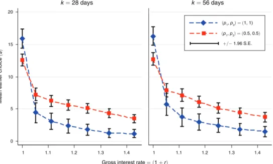
Section I provided a testable hypothesis for behavior across certain and uncertain intertemporal settings. For a given ( p1 , p2), if p1 = p2 < 1 then behavior should be identical to a similarly dated risk-free prospect, ( p1 = p2 = 1), at all gross interest rates, 1 + r, and all delay lengths, k. Figure 2 graphs aggregate behavior for the con-ditions ( p1 , p2) = (1,1) (diamonds) and ( p1 , p2) = (0.5,0.5) (squares) across the experimentally varied gross interest rates and delay lengths. The mean earlier choice of ct and a 95 percent confidence interval (+/−1.96 standard errors) are graphed.
Figure 1. Sample Decision Sheet 2006
Calendar S M T W Th F S
April
1 2 3 4
5 6 7 8 9 10 11
12 13 14 15 16 17 18 19 20 21 22 23 24 25 26 27 28 29 30
May
1 2
3 4 5 6 7 8 9
10 11 12 13 14 15 16 17 18 19 20 21 22 23 24 25 26 27 28 29 30 31
June
1 2 3 4 5 6
7 8 9 10 11 12 13 14 15 16 17 18 19 20 21 22 23 24 25 26 27 28 29 30
IN EACH ROW ALLOCATE 100 TOKENS BETWEEN
AND
PAYMENT A PAYMENT B
(1 week from today) (4 weeks later)
Date A:
April 8, 2009 May 6, 2009Date B:
Chance A Sent:
40% Chance 50%B Sent:
No. A Tokens Rate A
$ per token Date A
1. tokens at $0.20 each on April 8 tokens at $0.20 each on May 6
2. tokens at $0.19 each on April 8 tokens at $0.20 each on May 6
3. tokens at $0.18 each on April 8 tokens at $0.20 each on May 6
4. tokens at $0.17 each on April 8 tokens at $0.20 each on May 6
5. tokens at $0.16 each on April 8 tokens at $0.20 each on May 6
6. tokens at $0.15 each on April 8 tokens at $0.20 each on May 6
7. tokens at $0.14 each on April 8 tokens at $0.20 each on May 6
PLEASE MAKE SURE A + B TOKENS = 100 IN EACH ROW!
B Tokens Date B
& Rate B
$ per token &
& & & & &
Under DEU, preference-for-resolution models, and standard probability weight-ing behavior should be identical across the two conditions. We find strong evidence to the contrary. In a hypothesis test of equality across the two conditions, the overall difference is found to be highly significant: f14,79 = 6.07,p < 0.001.15
The data follow an interesting pattern. In ( p1 , p2) = (1,1) and (0.5,0.5) condi-tions, the allocation to sooner payments decrease as interest rates rise. At the lowest interest rate, however, ct allocations are substantially higher in the (1,1) condition,
and as the gross interest rate increases, (1,1) allocations drop steeply, crossing over the graph of the (0.5,0.5) condition.16 This crossover in behavior is in clear viola-tion of discounted expected utility, all models that reduce to discounted expected utility when uncertainty is immediately resolved, standard probability weighting, and temporally dependent probability weighting.
The aggregate violations of common ratio documented above are also supported in the individual data. Out of 14 opportunities to violate common ratio predictions,
15 Test statistic generated from nonparametric ordinary least squares (OLS) regression of choice on indicators for
interest rate (seven levels), delay length (two levels), risk condition (two levels) and all interactions with clustered standard errors. f-statistic corresponds to null hypothesis that all risk condition terms have zero slopes. See online Appendix Table A1 for regression.
16 Indeed, in the (1,1) condition, 80.7 percent of allocations are at one or the other budget corners while only
26.1 percent are corner solutions in the (0.5,0.5) condition. We interpret the corner solutions in the (1,1) condi-tion as evidence consistent with separability. See Andreoni and Sprenger (2012a) for a full discussion of censoring issues in CTBs. The difference in allocations across conditions is obtained for all sessions and for all orders indicat-ing no presence of order or day effects.
Figure 2. Aggregate Behavior under Certainty and Uncertainty
Notes: The figure presents aggregate behavior for N = 80 subjects under two conditions: ( p1 , p2) = (1,1), i.e., no
risk, (diamonds); and ( p1 , p2) = (0.5,0.5), i.e., 50 percent chance sooner payment would be sent and 50 percent
chance later payment would be sent, (squares); t = 7days in all cases, k ∈{28, 56} days. Error bars represent 95 percent confidence intervals, taken as +/−1.96 standard errors of the mean. Test of H0 :equality across conditions:
f14,79 = 6.07,p < 0.001.
0 5 10 15 20
1 1.1 1.2 1.3 1.4 1 1.1 1.2 1.3 1.4
k= 28 days k= 56 days
(p1, p2)=(1, 1)
(p1, p2)=(0.5, 0.5) +/− 1.96 S.E.
Mean earlier choice
(
$
)
individuals do so an average of 9.68 (standard deviation = 5.50) times. Only 15 per-cent of subjects (12 of 80) commit zero violations of expected utility. For the 85 per-cent of subjects who do violate expected utility, they do so in more than 80 perper-cent of opportunities, an average of 11.38 (standard deviation = 3.99) times. Figure 3, panel A presents a histogram of coun ti, each subject’s number of violations across condi-tions ( p1 , p2) = (1,1) and (0.5,0.5). More than 40 percent of subjects violate com-mon ratio predictions in all 14 opportunities. This may be a strict measure of violation as it requires identical allocation across risk conditions. As a complementary measure, we also present a histogram of | di |, the individual average budget share difference
Figure 3. Individual Behavior under Certainty and Uncertainty
Notes: The figure presents individual violations across three common ratio comparisons. The variable coun ti is a
count of each individual’s common ratio violations and di is each individual’s budget share difference between com-mon ratio conditions. Bin size for di is 0.04.
0 10 20 30 40 50
Percent
0 5 10 15
counti: Number of DEU violations
Percent
0 0.1 0.2 0.3 0.4 0.5 0.6
|di|: Individual budget share distance
Panel A. (p1, p2)=(1, 1) versus (0.5, 0.5)
Percent
0 5 10 15
counti: Number of DEU violations
Percent
di: Individual budget share distance
Panel B. (p1, p2)=(1, 0.8) versus (0.5, 0.4)
Percent
0 5 10 15
counti: Number of DEU violations
Percent
−0.6 −0.4 −0.2 0 0.2 0.4 0.6
di: Individual budget share distance
Panel C. (p1, p2)=(0.8, 1) versus (0.4, 0.5)
0 10 20 30 40 50
0 10 20 30 40 50
0 10 20 30 40 50
0 10 20 30 40 50 0 10 20 30 40 50
between risk conditions. For each individual and each CTB, we calculate the bud-get share of the sooner payment, (1 + r) ct/m. The average of each individual’s 14
budget share differences between common ratio conditions is the measure di. Here we consider the average absolute difference.17 The mean value of | d
i | is 0.27 (
stan-dard deviation = 0.18), indicating that individual violations are substantial, around 27 percent of the budget share. Indeed, 63.8 percent of the sample (51/80) exhibit |
di | > 0.2, indicating that violations are unlikely to be simple random response error. B. Behavior with Differential Risk
Next we explore the four conditions with differential risk. First, we discuss viola-tions of common ratio when only one payment is certain. Second, we examine the three conditions where all payments are uncertain and document behavior consistent with discounted expected utility.
A preference for Certainty.—Figure 4 compares behavior in four conditions with differential risk but common ratios of probabilities. Condition ( p1 , p2) = (1,0.8)( dia-monds) is compared to ( p1 , p2) = (0.5,0.4)(triangles), and condition ( p1 , p2) = (0.8,1)
(squares) is compared to ( p1 , p2) = (0.4,0.5) (crosses). The DEU model predicts equal allocations across conditions with common ratios. Interestingly, subjects’ allo-cations demonstrate a preference for certain payments relative to common ratio coun-terparts, regardless of whether the certain payment is sooner or later. Hypotheses of equal allocations across conditions are rejected in both cases.18
Panels B and C of Figure 3 demonstrate that the individual behavior is orga-nized in a similar manner. Individual violations of common ratio predictions are substantial. When certainty is sooner, across conditions ( p1 , p2) = (1,0.8) and ( p1 , p2) = (0.5,0.4), subjects commit an average of 10.90 (standard devia-tion = 4.67) common ratio violations in 14 opportunities and only 7.5 per-cent of subjects commit zero violations. The average distance in budget shares,
di, is 0.150 (standard deviation = 0.214), which is significantly greater than zero ( t79 = 6.24,p < 0.01), and in the direction of preferring the certain sooner payment. When certainty is later across conditions ( p1 , p2) = (0.8,1) and ( p1 , p2) = (0.4,0.5), subjects make an average of 9.68 (standard deviation = 5.74) common ratio viola-tions and 17.5 percent of subjects make no violaviola-tions at all, similar to panel A. The average distance in budget share, di, is − 0.161 (standard deviation = 0.198), which is significantly less than zero ( t79 = 7.27,p < 0.01), and in the direction of prefer-ring the certain later payment.
17 That is, the absolute value of each of the 14 differences is obtained prior to computing the average. When
computing di across comparisons ( p1 , p2) = (1,0.8) versus ( p1 , p2) = (0.5,0.4) and ( p1 , p2) = (0.8,1) and ( p1 , p2) = (0.4,0.5), the first budget share is subtracted from the second budget share to have a directional difference.
Relative to common ratio, a preference for certainty would be exhibited by a positive di across ( p1 , p2) = (1,0.8)
versus ( p1 , p2) = (0.5,0.4) and a negative di across ( p1 , p2) = (0.8,1) and ( p1 , p2) = (0.4,0.5). 18 For equality across ( p
1 , p2) = (1,0.8) and ( p1 , p2) = (0.5,0.4) f14,79 = 7.69,p < 0.001 and for equality
across ( p1 , p2) = (0.8,1) and ( p1 , p2) = (0.4,0.5) f14,79 = 5.46, p < 0.001. Test statistics generated from
non-parametric OLS regression of choice on indicators for interest rate (seven levels), delay length (two levels), risk condition (two levels), and all interactions with clustered standard errors. f-statistic corresponds to hypothesis that all risk condition terms have zero slopes. See online Appendix Table A1 for regression.
Importantly, violations of discounted expected utility correlate across experi-mental comparisons. Figure 5 plots budget share differences, di, across
common-ratio comparisons. The difference | di | from condition ( p1 , p2) = (1,1) versus
( p1 , p2) = (0.5,0.5) is on the vertical axis while di across the alternate
compari-sons is on the horizontal axis. Common ratio violations correlate highly across experimental conditions. The more an individual violates common ratio across conditions ( p1 , p2) = (1,1) and ( p1 , p2) = (0.5,0.5) predicts how much he or she will demonstrate a common ratio violation toward certainty when it is sooner in
( p1 , p2) = (1,0.8) versus ( p1 , p2) = (0.5,0.4), (ρ = 0.31,p < 0.01), and when it is later in ( p1 , p2) = (0.8,1) versus ( p1 , p2) = (0.4,0.5), (ρ = − 0.47,p < 0.01). Table 2 presents a correlation table for the number of violations coun ti, and the bud-get proportion differences di, across comparisons and shows significant individual
correlation across all conditions and measures of violation behavior.
These findings are critical for two reasons. First, the common ratio violations observed in this subsection could be predicted by a variety of formulations of prospect theory probability weighting (Kahneman and Tversky 1979; Tversky and Kahneman 1992; Tversky and Fox 1995; Wu and Gonzalez 1996; Prelec 1998; Gonzalez and Wu 1999; and Halevy 2008). Hence, the violations of DEU documented in this subsec-tion, unlike those of subsection IIIA, cannot reject a prospect theory interpretation to the data. Recognizing that violations correlate highly across contexts that can and cannot be explained by probability weighting suggests that prospect theory cannot
Figure 4. A Preference for Certainty
Notes: The figure presents aggregate behavior for N = 80 subjects under four conditions: ( p1 , p2) = (1,0.8), ( p1 , p2) = (0.5,0.4), ( p1 , p2) = (0.8,1), and ( p1 , p2) = (0.4,0.5). Error bars represent 95 percent confidence
intervals, taken as + /−1.96 standard errors of the mean. The first and second conditions share a common ratio as do the third and fourth. Test of H0 : equality across conditions ( p1 , p2) = (1,0.8) and ( p1 , p2) = (0.5,0.4):
f14,79 = 7.69,p < 0.001. Test of H0 : equality across conditions ( p1 , p2) = (0.8,1) and ( p1 , p2) = (0.4,0.5):
f14,79 = 5.46,p < 0.001. 0
5 10 15 20
0.8 1 1.2 1.4 1.6 1.8 0.8 1 1.2 1.4 1.6 1.8
(p1, p2)=(0.5, 0.4) (p1, p2)=(0.4, 0.5) +/− 1.96 S.E.
(p1, p2)=(1, 0.8) (p1, p2)=(0.8, 1)
Mean earlier choice
(
$
)
θ
k= 28 days k= 56 days
provide a unified account for the data. It is important to note, however, that pros-pect theory is primarily motivated for the study of decision-making under uncertainty. Clearly, more research analyzing prospect theory predictions in atemporal choices is required before conclusions can be drawn. In one recent example, Andreoni and Sprenger (2011) reach conclusions similar to those here in an atemporal environment.
Second, these results suggest strongly that a preference for certainty may play a critical role in generating dynamic inconsistencies. Here we have demonstrated that certain sooner payments are preferred over uncertain later payments in a way that is inconsistent with DEU at both the aggregate and individual levels. This phenomenon clearly did not involve intrinsic present bias because first, the present was not directly involved, and, second, the effect can be reversed by making later payments certain.
When All Choices Are Uncertain.—Figure 6 presents aggregate behavior from three risky situations: ( p1 , p2) = (0.5,0.5) (diamonds); ( p1 , p2) = (0.5,0.4) (squares); and ( p1 , p2) = (0.4,0.5)(triangles) over the experimentally varied values of θ and delay length. The mean earlier choice of ct is graphed along with error bars corre-sponding to 95 percent confidence intervals. We also plot predicted behavior based on structural discounting and utility estimates from the ( p1 , p2) = (0.5,0.5) data.19
19 Online Appendix B describes the estimation procedure, the methodology for which was developed in Andreoni
and Sprenger (2012a). Online Appendix B documents that a common set of parameters cannot simultaneously rationalize the ( p1 , p2) = (0.5,0.5) and ( p1 , p2) = (1,1) data. Online Appendix Table A2, column 6 provides
cor-Figure 5. Violation Behavior across Conditions
Notes: The figure presents the correlations of the budget share difference, di, across common ratio
compari-sons; | di | across conditions ( p1 , p2) = (1,1) and ( p1 , p2) = (0.5,0.5) is on the vertical axis; di across the
alter-nate comparisons is on the horizontal axis. Regression lines are provided. Corresponding correlation coefficients are ρ = 0.31, ( p < 0.01) for the triangular points ( p1 , p2) = (1,0.8) versus ( p1 , p2) = (0.5,0.4) and ρ = − 0.47, ( p < 0.01) for the circular points ( p1 , p2) = (0.8,1) versus ( p1 , p2) = (0.4,0.5). See Table 2 for more details.
0 0.2 0.4 0.6
|
di
|
(
1, 1
)
versus
(
0.5, 0.5
)
−0.6 −0.4 −0.2 0 0.2 0.4 0.6
di
(1, 0.8) versus (0.5, 0.4) Regression line
(0.8, 1) versus (0.4, 0.5) Regression line
These out-of-sample predictions are plotted as solid lines in green and orange. The solid red line corresponds to the model fit for ( p1 , p2) = (0.5,0.5).
We highlight two dimensions of Figure 6. First, the theoretical predictions are (i)
that ct should be declining in θ; and (ii) that if two decisions have identical θ then
ct should be higher in the condition with the lower interest rate.20 These features
are observed in the data. Allocations of ct decline with θ and, where overlap of θ exists, ct is generally higher for lower gross interest rates.21 Second, out-of-sample
predictions match actual aggregate behavior. Indeed, the out-of-sample calculated R2 values are high: 0.878 for ( p1 , p2) = (0.5,0.4) and 0.580 for ( p1 , p2) = (0.4,0.5).22
responding estimates based on the ( p1 , p2) = (0.5,0.5) and ( p1 , p2) = (1,1) data. In both conditions,
discount-ing is estimated to be around 30 percent per year. While substantial risk aversion is estimated from ( p1 , p2) = (0.5,0.5), limited utility function curvature is obtained when ( p1 , p2) = (1,1). Of interest is the close similarity
between the ( p1 , p2) = (1,1) estimates and those obtained in Andreoni and Sprenger (2012a), where payment risk
was minimized and no experimental variation of risk was implemented.
20 As discussed in Section I, c
t should be monotonically decreasing in θ. Additionally, if θ = θ′ and 1 + r≠ 1 + r′
then behavior should be identical up to a scaling factor related to the interest rates 1 + r and 1 + r′; ct should be
higher in the lower interest rate condition due to income effects.
21 This pattern of allocations is obtained for all sessions and for all orders indicating no presence of order or day
effects.
22 By comparison, making similar out-of-sample predictions using utility estimates from ( p
1 , p2) = (1,1) yields
predictions that diverge dramatically from actual behavior (see online Appendix Figure A2) and lowers R2 values
to 0.767 and 0.462, respectively. This suggests that accounting for differential utility function curvature in risky situations allows for an improvement of fit on the order of 15–25 percent.
Table 2—Individual Violation Correlation Table
counti counti counti | di| di di
(1, 1) (1, 0.8) (0.8, 1) (1, 1) (1, 0.8) (0.8, 1)
versus versus versus versus versus versus
(0.5, 0.5) (0.5, 0.4) (0.4, 0.5) (0.5, 0.5) (0.5, 0.4) (0.4, 0.5)
(1, 1)
counti versus 1
(0.5, 0.5) (1, 0.8)
counti versus 0.56*** 1 (0.5, 0.4)
(0.8, 1)
counti versus 0.71*** 0.72*** 1 (0.4, 0.5)
(1, 1)
| di| versus 0.84*** 0.40*** 0.52*** 1
(0.5, 0.5) (1, 0.8)
di versus 0.31*** 0.34*** 0.28** 0.31*** 1
(0.5, 0.4) (0.8, 1)
di versus −0.55*** −0.412*** −0.61*** −0.47*** −0.34*** 1
(0.4, 0.5)
Notes: Pairwise correlations with 80 observations. The variable coun t i is a count of each individual’s common ratio
violations, and d i is each individual’s budget share difference between common ratio conditions.
*** Significant at the 1 percent level.
** Significant at the 5 percent level.
Figure 6 demonstrates that in situations where all payments are risky, the results are surprisingly consistent with the DEU model. Though subjects exhibited a preference for certainty when it is available, away from certainty they trade off rela-tive risk and interest rates like expected utility maximizers, and utility parameters measured under uncertainty predict behavior out-of-sample extremely well.23
IV. Discussion and Conclusion
Intertemporal decision-making involves a combination of certainty and uncer-tainty. The present is known while the future is inherently risky. In an intertemporal allocation experiment under varying risk conditions, we document violations of dis-counted expected utility’s common-ratio predictions. Additionally, the pattern of results are inconsistent with various prospect theory probability-weighting formu-lations. Subjects exhibit a preference for certainty when it is available, but behave largely as discounted expected utility maximizers away from certainty.
23 Prospect theory probability weighting would make a similar prediction as many of the functional forms used
in the literature are near linear at intermediate probabilities (Kahneman and Tversky 1979; Tversky and Kahneman 1992; Tversky and Fox 1995; Wu and Gonzalez 1996; Prelec 1998; Gonzalez and Wu 1999).
Figure 6. Aggregate Behavior under Uncertainty
Notes: The figure presents aggregate behavior for N = 80 subjects under three conditions: ( p1 , p2) = (0.5,0.5), i.e.,
equal risk, (diamonds); ( p1 , p2) = (0.5,0.4), i.e., more risk later, (boxes); and ( p1 , p2) = (0.4,0.5), i.e., more risk
sooner, (triangles). Error bars represent 95 percent confidence intervals, taken as + /−1.96 standard errors of the mean. Solid lines correspond to predicted behavior using utility estimates from ( p1 , p2) = (0.5,0.5) as estimated in
online Appendix Table A2, column 6.
0 5 10 15 20
0.8 1 1.2 1.4 1.6 1.8 0.8 1 1.2 1.4 1.6 1.8
(p1, p2)=(0.5, 0.5) (0.5, 0.5) Fit
R2= 0.761
(0.5, 0.4) Prediction
R2= 0.878
(0.4,0.5) Prediction
R2= 0.580 +/− 1.96 S.E.
Mean earlier choice
(
$
)
k = 28 days k = 56 days
θ(1+ r)( p2/p
1)
Our results have substantial implications for intertemporal decision theory. In particular, present bias has been frequently documented (Frederick, Loewenstein, and O’Donoghue 2002) and is argued to be a dynamically inconsistent discounting phenomenon generated by diminishing impatience through time. Our results sug-gest that present bias may have an alternate source. If individuals exhibit a prefer-ence for certainty when it is available, then present certain consumption will be favored over future uncertain consumption. When only uncertain future consump-tion is considered, individuals act more closely in line with expected utility and apparent preference reversals are generated.
Other research has discussed the possibility that certainty plays a role in generating present bias (Halevy 2008). Additionally, such a notion is implicit in the recognized dynamic inconsistency of nonexpected utility models (Green 1987, and Machina 1989), and could be thought of as preferring immediate resolution of uncertainty
(Kreps and Porteus 1978; Chew and Epstein 1989; and Epstein and Zin 1989). Our results point in a new direction: that certainty, per se, may be disproportionately pre-ferred. We interpret our findings as being consistent with the intuition of the Allais Paradox (Allais 1953). Allais (1953) argued that when two options are far from certain, individuals act effectively as discounted expected utility maximizers, while when one option is certain and another is uncertain, a disproportionate preference for certainty prevails. This intuition is captured closely in the u–v preference models of Neilson (1992); Schmidt (1998); and Diecidue, Schmidt, and Wakker (2004), predicting that the observed behavior across our experimental conditions is a feature of belief-dependent utility (Dufwenberg 2008) and expectations-based reference dependence (Bell 1985; Loomes and Sugden 1986; and K ˝ o szegi and Rabin 2006, 2007), and may help researchers to understand the origins of dynamic inconsistency, build sharper theoretical models, provide richer experimental tests, and form more careful policy prescriptions regarding intertemporal choice.
REFERENCES
Allais, Maurice. 1953. “Le Comportement de l’Homme Rationnel devant le Risque: Critique des Pos-tulats et Axiomes de l’Ecole Americaine.” Econometrica 21 (4): 503–46.
Andersen, Steffen, James C. Cox, Glenn W. Harrison, Morten I. Lau, E. Elisabet Rutström, and Vjollca Sadiraj. 2011. “Asset Integration and Attitudes to Risk: Theory and Evidence.” Unpublished. Andersen, Steffen, Glenn W. Harrison, Morten I. Lau, and E. Elisabet Rutström. 2008. “Eliciting Risk
and Time Preferences.” Econometrica 76 (3): 583–618.
Andreoni, James, and Charles Sprenger. 2011. “Uncertainty Equivalents: Testing the Limits of the Independence Axiom.” Unpublished.
Andreoni, James, and Charles Sprenger. 2012a. “Estimating Time Preferences from Convex Budgets.”
American Economic Review. 102 (7): 3333–56.
Andreoni, James, and Charles Sprenger. 2012b. “Risk Preferences Are Not Time Preferences: Data-set.” American Economic Review. http://dx.doi.org/10.1257/aer.102.7.3357.
Baucells, Manel, and Franz H. Heukamp. 2010. “Common Ratio Using Delay.” Theory and Decision 68 (1-2): 149–58.
Bell, David E. 1985. “Disappointment in Decision Making under Uncertainty.” Operations Research 33 (1): 1–27.
Boyarchenko, Svetlana, and Sergei Levendorskii. 2010. “Discounting When Income is Stochastic and Climate Change Policies.” Unpublished.
Camerer, Colin F. 1992. “Recent Tests of Generalizations of Expected Utility Theory.” In Utility
The-ories: Measurements and Applications, edited by Ward Edwards, 207–51. Dordrecht, Netherlands: Kluwer Academic.
Chew, Soo Hong. 1989. “Axiomatic Utility Theories with the Betweenness Property.” Annals of
Opera-tions Research 19 (1): 273–98.
Chew, Soo Hong, and Larry G. Epstein. 1989. “The Structure of Preferences and Attitudes towards the Timing of the Resolution of Uncertainty.” International Economic Review 30 (1): 103–17.
Coller, Maribeth, and Melonie B. Williams. 1999. “Eliciting Individual Discount Rates.” Experimental
Economics 2 (2): 107–27.
Dekel, Eddie. 1986. “An Axiomatic Characterization of Preferences under Uncertainty: Weakening the Independence Axiom.” Journal of Economic Theory 40 (2): 304–18.
Diecidue, Enrico, Ulrich Schmidt, and Peter P. Wakker. 2004. “The Utility of Gambling Reconsid-ered.” Journal of Risk and Uncertainty 29 (3): 241–59.
Dufwenberg, Martin. 2008. “Psychological Games.” In The New palgrave Dictionary of Economics, edited by Steven N. Durlauf and Lawrence E. Blume. New york: Palgrave Macmillan.
Ellingsen, Tore. 1994. “Cardinal Utility: A History of Hedonimetry.” In Cardinalism: A fundamental
Approach, edited by Maurice Allais and Ole Hagen, 105–65. Dordrecht, Netherlands: Kluwer Aca-demic Publishers.
Epstein, Larry G., and Stanley E. Zin. 1989. “Substitution, Risk Aversion, and the Temporal Behav-ior of Consumption and Asset Returns: A Theoretical Framework.” Econometrica 57 (4): 937–69. Frederick, Shane, George Loewenstein, and Ted O'Donoghue. 2002. “Time Discounting and Time
Preference: A Critical Review.” Journal of Economic Literature 40 (2): 351–401.
Giné, Xavier, Jessica Goldberg, Dan Silverman, and Dean Yang. 2010. “Revising Commitments: Time Preference and Time-Inconsistency in the Field.” Unpublished.
Gneezy, Uri, John A. List, and George Wu. 2006. “The Uncertainty Effect: When a Risky Prospect Is Valued Less Than Its Worst Possible Outcome.” Quarterly Journal of Economics 121 (4): 1283–309. Gonzalez, Richard, and George Wu. 1999. “On the Shape of the Probability Weighting Function.”
Cognitive psychology 38 (1): 129–66.
Green, Jerry. 1987. “‘Making Book against Oneself,’ the Independence Axiom, and Nonlinear Utility Theory.” Quarterly Journal of Economics 102 (4): 785–96.
Halevy, Yoram. 2008. “Strotz Meets Allais: Diminishing Impatience and the Certainty Effect.”
Ameri-can Economic Review 98 (3): 1145–62.
Harless, David W., and Colin F. Camerer. 1994. “The Predictive Utility of Generalized Expected Util-ity Theories.” Econometrica 62 (6): 1251–89.
Harrison, Glenn W., Morten Igel Lau, E. Elisabet Rutström, and Melonie B. Sullivan. 2005. “Elicit-ing Risk and Time Preferences Us“Elicit-ing Field Experiments: Some Methodological Issues.” In field
Experiments in Economics, edited by Jeffrey P. Carpenter, Glenn W. Harrison, and John A. List, 125–218. Amsterdam: Elsevier.
Harrison, Glenn W., Morten I. Lau, and Melonie B. Williams. 2002. “Estimating Individual Discount Rates in Denmark: A Field Experiment.” American Economic Review 92 (5): 1606–17.
Kahneman, Daniel, and Amos Tversky. 1979. “Prospect Theory: An Analysis of Decision under Risk.”
Econometrica 47 (2): 263–91.
Keren, Gideon, and Peter Roelofsma. 1995. “Immediacy and Certainty in Intertemporal Choice.”
Organizational Behavior and Human Decision processes 63 (3): 287–97.
K ˝ o szegi, Botond, and Matthew Rabin. 2006. “A Model of Reference-Dependent Preferences.”
Quar-terly Journal of Economics 121 (4): 1133–65.
K ˝ o szegi, Botond, and Matthew Rabin. 2007. “Reference-Dependent Risk Attitudes.” American
Eco-nomic Review 97 (4): 1047–73.
Kreps, David M., and Evan L. Porteus. 1978. “Temporal Resolution of Uncertainty and Dynamic Choice Theory.” Econometrica 46 (1): 185–200.
Laibson, David. 1997. “Golden Eggs and Hyperbolic Discounting.” Quarterly Journal of Economics 112 (2): 443–77.
Loewenstein, George, and Drazen Prelec. 1992. “Anomalies in Intertemporal Choice: Evidence and an Interpretation.” Quarterly Journal of Economics 107 (2): 573–97.
Loewenstein, George, and Richard H. Thaler. 1989. “Intertemporal Choice.” Journal of Economic
per-spectives 3 (4): 181–93.
Loomes, Graham, and Robert Sugden. 1986. “Disappointment and Dynamic Consistency in Choice under Uncertainty.” Review of Economic Studies 53 (2): 271–82.
Machina, Mark J. 1989. “Dynamic Consistency and Non-expected Utility Models of Choice under Uncertainty.” Journal of Economic Literature 27 (4): 1622–68.
Neilson, William S. 1992. “Some Mixed Results on Boundary Effects.” Economics Letters 39 (3): 275–78.
O’Donoghue, Ted, and Matthew Rabin. 1999. “Doing It Now or Later.” American Economic Review 89 (1): 103–24.
Onay, Selcuk, and Ayse Onculer. 2007. “Intertemporal Choice under Timing Risk: An Experimental Approach.” Journal of Risk and Uncertainty 34 (2): 99–121.
Prelec, Drazen. 1998. “The Probability Weighting Function.” Econometrica 66 (3): 497–527. Quiggin, John. 1982. “A Theory of Anticipated Utility.” Journal of Economic Behavior and
Organiza-tion 3 (4): 323–43.
Samuelson, P. A. 1937. “A Note on Measurement of Utility.” Review of Economic Studies 4: 155–61. Schmidt, Ulrich. 1998. “A Measurement of the Certainty Effect.” Journal of Mathematical
psychol-ogy 42 (1): 32–47.
Starmer, Chris. 2000. “Developments in Non-expected Utility Theory: The Hunt for a Descriptive Theory of Choice under Risk.” Journal of Economic Literature 38 (2): 332–82.
Starmer, Chris, and Robert Sugden. 1991. “Does the Random-Lottery Incentive System Elicit True Preferences? An Experimental Investigation.” American Economic Review 81 (4): 971–78. Tversky, Amos, and Craig R. Fox. 1995. “Weighing Risk and Uncertainty.” psychological Review 102
(2): 269–83.
Tversky, Amos, and Daniel Kahneman. 1992. “Advances in Prospect Theory: Cumulative Representa-tion of Uncertainty.” Journal of Risk and Uncertainty 5 (4): 297–323.
Weber, Bethany J., and Gretchen B. Chapman. 2005. “The Combined Effects of Risk and Time on Choice: Does Uncertainty Eliminate the Immediacy Effect? Does Delay Eliminate the Certainty Effect?” Organizational Behavior and Human Decision processes 96 (2): 104–18.
Wu, George, and Richard Gonzalez. 1996. “Curvature of the Probability Weighting Function.”