12.1 Introduction
This chapter introduces finite-state machines, a primitive, but useful computational model for both hardware and certain types of software. We also discuss regular expressions, the correspondence between non-deterministic and deterministic machines, and more on grammars. Finally, we describe typical hardware components that are essentially physical realizations of finite-state machines.
Finite-state machines provide a simple computational model with many applications. Recall the definition of a Turing machine: a finite-state controller with a movable read/write head on an unbounded storage tape. If we restrict the head to move in only one direction, we have the general case of a finite-state machine. The sequence of symbols being read can be thought to constitute the input, while the sequence of symbols being written could be thought to constitute the output. We can also derive output by looking at the internal state of the controller after the input has been read.
Finite-state machines, also called finite-state automata (singular: automaton) or just finite automata are much more restrictive in their capabilities than Turing machines. For example, we can show that it is not possible for a finite-state machine to determine whether the input consists of a prime number of symbols. Much simpler languages, such as the sequences of well-balanced parenthesis strings, also cannot be recognized by finite-state machines. Still there are the following applications:
• Simple forms of pattern matching (precisely the patterns definable by "regular expressions”, as we shall see).
• Models for sequential logic circuits, of the kind on which every present-day computer and many device controllers is based.
• An intimate relationship with directed graphs having arcs labeled with symbols from the input alphabet.
Even though each of these models can be depicted in a different setting, they have a common mathematical basis. The following diagram shows the context of finite-state machines among other models we have studied or will study.
Finite-State Machines, Finite-State Automata Turing Machines
Finite-State Grammars Context-Free Grammars
Regular Expressions, Regular Languages Finite Directed
Labelled Graphs Combinational
Logic Switching Circuits Sequential Logic Switching Circuits
Figure 189: The interrelationship of various models with respect to computational or representational power.
The arrows move in the direction of restricting power. The bi-directional arrows show equivalences.
Finite-State Machines as Restricted Turing Machines
One way to view the finite-state machine model as a more restrictive Turing machine is to separate the input and output halves of the tapes, as shown below. However, mathematically we don't need to rely on the tape metaphor; just viewing the input and output as sequences of events occurring in time would be adequate.
q
Input to be read Output written so far
Direction of head motion
Figure 190: Finite-state machine as a one-way moving Turing machine
q
Input to be read
Output written so far
Direction of head motion
q
Direction of tape motion
Direction of tape motion
reading writing
Figure 192: Finite-state machine viewed as a stationary-head, moving-tape, device
Since the motion of the head over the tape is strictly one-way, we can abstract away the idea of a tape and just refer to the input sequence read and the output sequence produced, as suggested in the next diagram. A machine of this form is called a transducer, since it maps input sequences to output sequences. The term Mealy machine, after George H. Mealy (1965), is also often used for transducer.
Input sequence Output sequence
Finite set of internal states
x x x x ...1 2 3 4 y y y y ...
1 2 3 4
Figure 193: A transducer finite-state machine viewed as a tapeless "black box" processing an input sequence to produce an output sequence
On the other hand, occasionally we are not interested in the sequence of outputs produced, but just an output associated with the current state of the machine. This simpler model is called a classifier, or Moore machine, after E.F. Moore (1965).
Input sequence
Finite set of internal states
x x x x ... 1 2 3 4 Output
associated with current state
z
Figure 194: Classifier finite-state machine.
Modeling the Behavior of Finite-State Machines
Concentrating initially on transducers, there are several different notations we can use to capture the behavior of finite-state machines:
• As a functional program mapping one list into another.
• As a restricted imperative program, reading input a single character at a time and producing output a single character at a time.
• As a feedback system.
• Representation of functions as a table
• Representation of functions by a directed labeled graph
For concreteness, we shall use the sequence-to-sequence model of the machine, although the other models can be represented similarly. Let us give an example that we can use to show the different notations:
Example: An Edge-Detector
The function of an edge detector is to detect transitions between two symbols in the input sequence, say 0 and 1. It does this by outputting 0 as long as the most recent input symbol is the same as the previous one. However, when the most recent one differs from the previous one, it outputs a 1. By convention, the edge detector always outputs 0 after reading the very first symbol. Thus we have the following input output sequence pairs for the edge-detector, among an infinite number of possible pairs:
input output
0 0
00 00
01 01
011 010
0111 0100
01110 01001
1 0
10 01
101 011
1010 0111
10100 01110
Functional Program View of Finite-State Machines
In this view, the behavior of a machine is as a function from lists to lists. Each state of the machine is identified with such a function.
The initial state is identified with the overall function of the machine.
The functions are interrelated by mutual recursion: when a function processes an input symbol, it calls another function to process the remaining input.
Each function:
looks at its input by one application of first,
produces an output by one application of cons, the first argument of which is determined purely by the input obtained from first, and
calls another function (or itself) on rest of the input. We make the assumptions that:
The result of cons, in particular the first argument, becomes partially available even before its second argument is computed.
Each function will return NIL if the input list is NIL, and we do not show this explicitly.
Functional code example for the edge-detector:
We will use three functions, f, g, and h. The function f is the overall representation of the
edge detector.
f([0 | Rest]) => [0 | g(Rest)]; f([1 | Rest]) => [0 | h(Rest)]; f([]) => [];
g([0 | Rest]) => [0 | g(Rest)]; g([1 | Rest]) => [1 | h(Rest)]; g([]) => [];
h([0 | Rest]) => [1 | g(Rest)]; h([1 | Rest]) => [0 | h(Rest)]; h([]) => [];
Notice that f is never called after its initial use. Its only purpose is to provide the proper
Example of f applied to a specific input:
f([0, 1, 1, 1, 0]) ==> [0, 1, 0, 0, 1]
An alternative representation is to use a single function, say k, with an extra argument,
treated as just a symbol. This argument represents the name of the function that would have been called in the original representation. The top-level call to k will give the initial
state as this argument:
k("f", [0 | Rest]) => [0 | k("g", Rest)]; k("f", [1 | Rest]) => [0 | k("h", Rest)]; k("f", []) => [];
k("g", [0 | Rest]) => [0 | k("g", Rest)]; k("g", [1 | Rest]) => [1 | k("h", Rest)]; k("g", []) => [];
k("h", [0 | Rest]) => [1 | k("g", Rest)]; k("h", [1 | Rest]) => [0 | k("h", Rest)]; k("h", []) => [];
The top level call with input sequence x is k("f", x) since "f" is the initial state.
Imperative Program View of Finite-State Machines
In this view, the input and output are viewed as streams of characters. The program repeats the processing cycle:
read character, select next state, write character, go to next state
ad infinitum. The states can be represented as separate "functions", as in the functional view, or just as the value of one or more variables. However the allowable values must be restricted to a finite set. No stacks or other extendible structures can be used, and any arithmetic must be restricted to a finite range.
The following is a transliteration of the previous program to this view. The program is started by calling f(). Here we assume that read() is a method that returns the next
character in the input stream and write(c) writes character c to the output stream.
void f() // initial function
{
switch( read() ) {
case '0': write('0'); g(); break; case '1': write('0'); h(); break; }
}
void g() // previous input was 0 {
switch( read() ) {
case '0': write('0'); g(); break;
case '1': write('1'); h(); break; // 0 -> 1 transition }
}
void h() // previous input was 1 {
switch( read() ) {
case '0': write('1'); g(); break; // 1 -> 0 transition case '1': write('0'); h(); break;
} }
[Note that this is a case where all calls can be "tail recursive", i.e. could be implemented as gotos by a smart compiler.]
The same task could be accomplished by eliminating the functions and using a single variable to record the current state, as shown in the following program. As before, we assume read() returns the next character in the input stream and write(c) writes
character c to the output stream.
static final char f = 'f'; // set of states
static final char g = 'g'; static final char h = 'h';
static final char initial_state = f; main()
{
char current_state, next_state; char c;
while( (c = read()) != EOF ) {
switch( current_state ) {
case f: // initial state switch( c )
{
case '0': write('0'); next_state = g; break; case '1': write('0'); next_state = h; break; }
break;
case g: // last input was 0 switch( c )
{
case '0': write('0'); next_state = g; break;
case '1': write('1'); next_state = h; break; // 0 -> 1 }
break;
case h: // last input was 1 switch( c )
{
case '0': write('1'); next_state = g; break; // 1 -> 0 case '1': write('0'); next_state = h; break;
} break; }
current_state = next_state; }
}
Feedback System View of Finite-State Machines
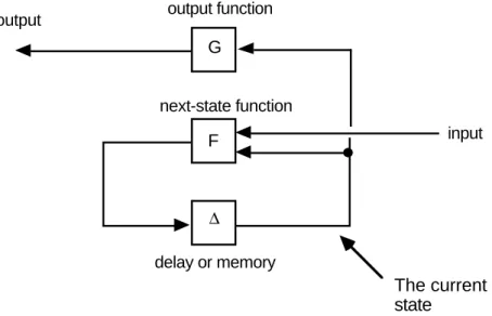
The feedback system view abstracts the functionality of a machine into two functions, the next-state or state-transition function F, and the output function G.
F: States
x
Symbols → States state-transition function G: Statesx
Symbols → Symbols output functionThe meaning of these functions is as follows:
F(q,
σ
) is the state to which the machine goes when currently in state q andσ
is read G(q,σ
) is the output produced when the machine is currently in state q andσ
is read The relationship of these functions is expressible by the following diagram.G
F
∆
output function
next-state function
delay or memory output
input
The current state
Figure 195: Feedback diagram of finite-state machine structure
From F and G, we can form two useful functions
F*: States
x
Symbols* → States extended state-transition function G*: Statesx
Symbols* → Symbols extended output functionwhere Symbols* denotes the set of all sequences of symbols. This is done by induction: F*(q, λ) = q
F*(q, xσ) = F(F*(q, x), σ ) G*(q, λ) = λ
G*(q, xσ) = G*(q, x) G(F*(q, x), σ )
In the last equation, juxtaposition is like cons’ing on the right. In other words, F*(q, x) is the state of the machine after all symbols in the sequence x have been processed, whereas G*(q, x) is the sequence of outputs produced along the way. In essence, G* can be regarded as the function computed by a transducer. These definitions could be transcribed into rex rules by representing the sequence xσ as a list [σ | x] with λ corresponding to [ ].
Tabular Description of Finite-State Machines
This description is similar to the one used for Turing machines, except that the motion is left unspecified, since it is implicitly one direction. In lieu of the two functions F and G, a
finite-state machine could be specified by a single function combining F and G of the form:
States
x
Symbols → Statesx
Symbolsanalogous to the case of a Turing machine, where we included the motion: States
x
Symbols → Symbolsx
Motionsx
StatesThese functions can also be represented succinctly by a table of 4-tuples, similar to what we used for a Turing machine, and again called a state transition table:
State1, Symbol1, State2, Symbol2
Such a 4-tuple means the following:
If the machine's control is in State1 and reads Symbol1, then machine will write Symbol2 and the next state of the controller will be State2.
The state-transition table for the edge-detector machine is:
current state input symbol next state output symbol
start state f 0 g 0
f 1 h 0
g 0 g 0
g 1 h 1
h 0 g 1
h 1 h 0
Unlike the case of Turing machines, there is no particular halting convention. Instead, the machine is always read to proceed from whatever current state it is in. This does not stop us from assigning our own particular meaning of a symbol to designate, for example, end-of-input.
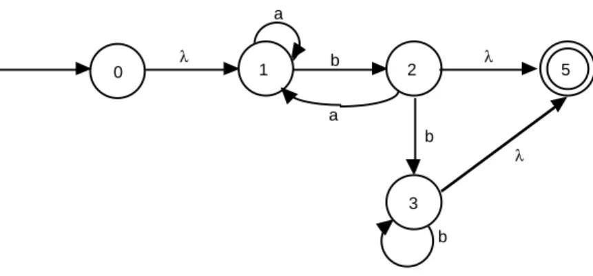
Classifiers, Acceptors, Transducers, and Sequencers
In some problems we don't care about generating an entire sequence of output symbols as do the transducers discussed previously. Instead, we are only interested in categorizing each input sequence into one of a finite set of possibilities. Often these possibilities can be made to derive from the current state. So we attach the result of the computation to the state, rather than generate a sequence. In this model, we have an output function
which gives a category or class for each state. We call this type of machine a classifier or
controller. We will study the conrtoller aspect further in the next chapter. For now, we
focus on the classification aspect. In the simplest non-trivial case of classifier, there are two categories. The states are divided up into the "accepting" states (class 1, say) and the "rejecting" states (class 0). The machine in this case is called an acceptor or recognizer. The sequences it accepts are those given by
c(F*(q0, x)) = 1
that is, the sequences x such that, when started in state q0, after reading x, the machine is in a state q such that c(q) = 1. The set of all such x, since it is a set of strings, is a
language in the sense already discussed. If A designates a finite-state acceptor, then
L(A) = { x in
Σ
* | c(F*(q0, x)) = 1} is the language accepted by A.The structure of a classifier is simpler than that of a transducer, since the output is only a function of the state and not of both the state and input. The structure is shown as follows:
G
F
∆
output function
next-state function
delay or memory output
input
The current state
Figure 196: Feedback diagram of classifier finite-state machine structure
A final class of machine, called a sequencer or generator, is a special case of a transducer or classifier that has a single-letter input alphabet. Since the input symbols are unchanging, this machine generates a fixed sequence, interpreted as either the output sequence of a transducer or the sequence of classifier outputs. An example of a sequencer is a MIDI (Musical Instrument Digital Interface) sequencer, used to drive electronic musical instruments. The output alphabet of a MIDI sequencer is a set of 16-bit words, each having a special interpretation as pitch, note start and stop, amplitude, etc. Although
most MIDI sequencers are programmable, the program typically is of the nature of an initial setup rather than a sequential input.
Description of Finite-State Machines using Graphs
Any finite-state machine can be shown as a graph with a finite set of nodes. The nodes correspond to the states. There is no other memory implied other than the state shown. The start state is designated with an arrow directed into the corresponding node, but otherwise unconnected.
Figure 197: An unconnected in-going arc indicates that the node is the start state
The arcs and nodes are labeled differently, depending on whether we are representing a transducer, a classifier, or an acceptor. In the case of a transducer, the arcs are labeled
σ/δ
as shown below, whereσ
is the input symbol andδ
is the output symbol. The state-transition is designated by virtue of the arrow going from one node to another.σ/δ
1 q
2 q
Figure 198: Transducer transition from q1 to q2, based on input
σ
, giving outputδ
In the case of a classifier, the arrow is labeled only with the input symbol. The categories are attached to the names of the states after /.
q / c
1 1 q / c2 2
σ
Figure 199: Classifier transition from q1 to q2, based on input
σ
In the case of a acceptor, instead of labeling the states with categories 0 and 1, we sometimes use a double-lined node for an accepting state and a single-lined node for a rejecting state.
a
q
Figure 200: Acceptor, an accepting state
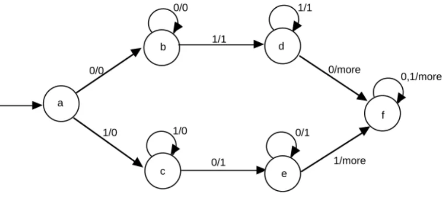
Transducer Example
The edge detector is an example of a transducer. Here is its graph:
f g
h
0/0
1/0 0/1
1/1
0/0
1/0
Figure 201: Directed labeled graph for the edge detector
Let us also give examples of classifiers and acceptors, building on this example.
Classifier Example
Suppose we wish to categorize the input as to whether the input so far contains 0, 1, or more than 1 "edges" (transitions from 0 to 1, or 1 to 0). The appropriate machine type is classifier, with the outputs being in the set {0, 1, more}. The name "more" is chosen arbitrarily. We can sketch how this classifier works with the aid of a graph.
The construction begins with the start state. We don't know how many states there will be initially. Let us use a, b, c, ... as the names of the states, with a as the start state. Each state is labeled with the corresponding class as we go. The idea is to achieve a finite closure after some number of states have been added. The result is shown below:
b/0 0
1
c/0
d/1 0
a/0
1
1
e/1 0
f / more
1
0
1
0 0, 1
Figure 202: Classifier for counting 0, 1, or more than 1 edges
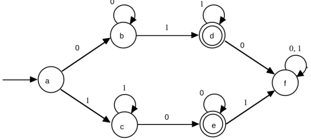
Acceptor Example
Let us give an acceptor that accepts those strings with exactly one edge. We can use the state transitions from the previous classifier. We need only designate those states that categorize there being one edge as accepting states and the others as rejecting states.
b 0
1
c
d 0
a
1
1
e 0
f
1
0
1
0 0, 1
Sequencer Example
The following sequencer, where the sequence is that of the outputs associated with each state, is that for a naive traffic light:
q0 /
green q1 / yellow
q2 / red
Figure 204: A traffic light sequencer
Exercises
1 •• Consider a program that scans an input sequence of characters to determine whether the sequence as scanned so far represents either an integer numeral, a floating-point numeral, unknown, or neither. As it scans each character, it outputs the corresponding assessment of the input. For example,
Input Scanned Assessment
1 integer
+ unknown
+1 integer
+1. floating-point
1.5 floating-point
1e unknown
1e-1 floating-point
1e. neither
Describe the scanner as a finite-state transducer using the various methods presented in the text.
2 •• Some organizations have automated their telephone system so that messages can be sent via pushing the buttons on the telephone. The buttons are labeled with both numerals and letters as shown:
1
2
a b c
3
d e f
4
g h i
5
j k l
6
m n o
7
p r s
8
t u v
9
w x y
*
0
#
Notice that certain letters are omitted, presumably for historical reasons. However, it is common to use * to represent letter q and # to represent letter z. Common schemes do not use a one-to-one encoding of each letter. However, if we wanted such an encoding, one method would be to use two digits for each letter:
The first digit is the key containing the letter.
The second digit is the index, 1, 2, or 3, of the letter on the key. For example, to send the word "cat", we'd punch:
2 3 2 1 8 1 c a t
An exception would be made for 'q' and 'z', as the only letters on the keys '*' and '#' respectively.
Give the state-transition table for communicating a series of any of the twenty-six letters, where the input alphabet is the set of digits {1, ...., 9, *, #} and the output alphabet is the set of available letters. Note that outputs occur only every other input. So we need a convention for what output will be shown in the transducer in case there is no output. Use λ for this output.
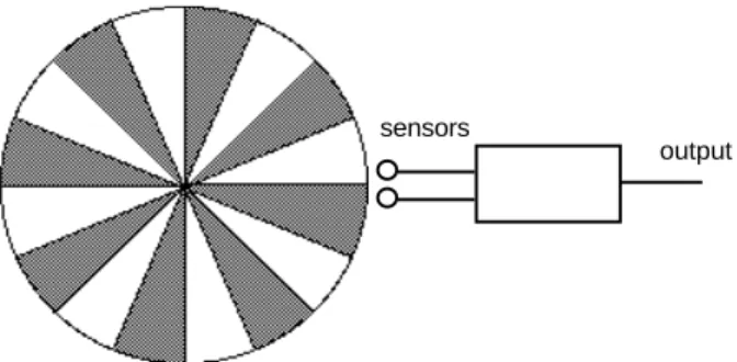
3 •• The device sketched below is capable of partially sensing the direction (clockwise, counterclockwise, or stopped) of a rotating disk, having sectors painted alternating gray and white. The two sensors, which are spaced so as to fit well within a single sector, regularly transmit one of four input possibilities: wg (white-gray), ww (white-white), gw (gray-white), and gg (gray-gray). The sampling rate must be fast enough, compared with the speed of the disk, that artifact readings do not take place. In other words, there must be at least one sample taken every time the disk moves from one of the four input combinations to another. From the transmitted input values, the device produces the directional
information. For example, if the sensors received wg (as shown), then ww for awhile, then gw, it would be inferred that the disk is rotating clockwise. On the other hand, if it sensed gw more than once in a row, it would conclude that the disk has stopped. If it can make no other definitive inference, the device will indicate its previous assessment. Describe the device as a finite-state transducer, using the various methods presented in the text.
sensors
output
Figure 205: A rotational direction detector
4 •• Decide whether the wrist-watch described below is best represented as a classifier or a transducer, then present a state-transition diagram for it. The watch has a chronograph feature and is controlled by three buttons, A, B, and C. It has three display modes: the time of day, the chronograph time, and "split" time, a saved version of the chronograph time. Assume that in the initial state, the watch displays time of day. If button C is pressed, it displays chronograph time. If C is pressed again, it returns to displaying time of day. When the watch is displaying chronograph time or split time, pressing A starts or stops the chronograph. Pressing B when the chronograph is running causes the chronograph time to be recorded as the split time and displayed. Pressing B again switches to displaying the chronograph. Pressing B when the chronograph is stopped resets the chronograph time to 0.
5 ••• A certain vending machine vends soft drinks that cost $0.40. The machine accepts coins in denominations of $0.05, $0.10, and $0.25. When sufficient coins have been deposited, the machine enables a drink to be selected and returns the appropriate change. Considering each coin deposit and the depression of the drink button to be inputs, construct a state-transition diagram for the machine. The outputs will be signals to vend a drink and return coins in selected denominations. Assume that once the machine has received enough coins to vend a drink, but the vend button has still not been depressed, that any additional coins will just be returned in kind. How will your machine handle cases such as the sequence of coins 10, 10, 10, 5, 25?
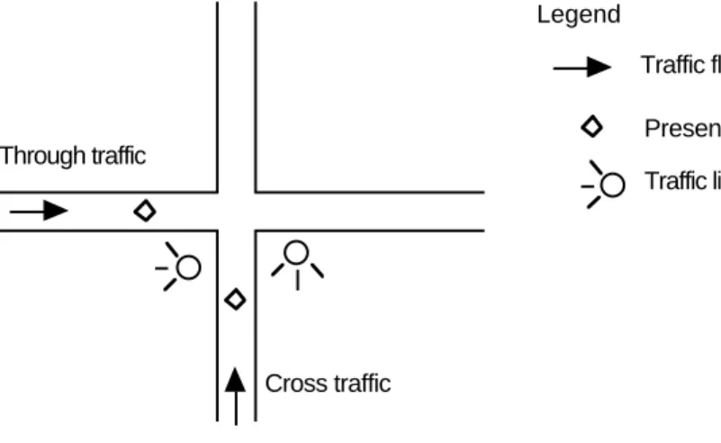
6 ••• Consider the problem of controlling traffic at an intersection such as shown below.
Legend
Traffic flow direction Presence sensor Traffic light Through traffic
Cross traffic
Figure 206: A traffic intersection
Time is divided into equal-length intervals, with sensors sampling the presence of traffic just before the end of an interval. The following priority rules apply:
1. If no traffic is present, through-traffic has the right-of-way.
2. If through-traffic is still present at the end of the first interval during which through-traffic has had the right-of-way, through-traffic is given the right-of-way one additional interval.
3. If cross-traffic is present at the end of the second consecutive interval during which through-traffic has had the right-of-way, then cross-traffic is given the right-of-way for one interval.
4. If cross-traffic is present but through-traffic is absent, cross-traffic maintains the right-of-way until an interval in which through-traffic appears, then through-traffic is given the right-of-way.
Describe the traffic controller as a classifier that indicates which traffic has the right-of-way.
7 ••• A bar code represents bits as alternating light and dark bands. The light bands are of uniform width, while the dark bands have width either equal to, or double, the width of the light bands. Below is an example of a code-word using the bar code. The tick marks on top show the single widths.
Figure 207: A bar code scheme
Assume that a bar-code reader translates the bands into symbols, L for light, D for dark, one symbol per single width. Thus the symbol sequence for the code-word above would be
L D L D D L D D L D L D D L D L
A bar pattern represents a binary sequence as follows: a 0 is encoded as LD, while a 1 is encoded as LDD. A finite-state transducer M can translate such a code into binary. The output alphabet for the transducer is {0, 1, _, end}. When started in its initial state, the transducer will "idle" as long as it receives only L's. When it receives its first D, it knows that the code has started. The transducer will give output 0 or 1 as soon it has determined the next bit from the bar pattern. If the bit is not known yet, it will give output _. Thus for the input sequence above, M will produce
_ _ 0 _ 1 _ _ 1 _ _ 0 _ 1 _ _ 0 L D L D D L D D L D L D D L D L
where we have repeated the input below the output for convenience. The transducer will output the symbol end when it subsequently encounters two L's in a row, at which point it will return to its initial state.
a. Give the state diagram for transducer M, assuming that only sequences of the indicated form can occur as input.
b. Certain input sequences should not occur, e.g. L D D D. Give a state-transition diagram for an acceptor A that accepts only the sequences corresponding to a valid bar code.
8 •• A gasoline pump dispenses gas based on credit card and other input from the customer. The general sequence of events, for a single customer is:
Customer swipes credit card through the slot.
Customer enters PIN (personal identification number) on keypad, with appropriate provisions for canceling if an error is made.
Customer removes nozzle. Customer lifts pump lever.
Customer squeezes or releases lever on nozzle any number of times. Customer depresses pump lever and replaces nozzle.
Customer indicates whether or not a receipt is wanted.
Sketch a state diagram for modeling such as system as a finite-state machine.
Inter-convertibility of Transducers and Classifiers (Advanced)
We can describe a mathematical relationship between classifiers and transducers, so that most of the theory developed for one will be applicable to the other. One possible connection is, given an input sequence x, record the outputs corresponding to the states through which a classifier goes in processing x. Those outputs could be the outputs of an appropriately-defined transducer. However, classifiers are a little more general in this sense, since they give output even for the empty sequence
λ
, whereas the output for a transducer with inputλ
is always justλ
. Let us work in terms of the following equivalence:A transducer T started in state q0 is equivalent to a classifier C started in state q0 if, for any non-empty sequence x, the sequence of outputs emitted by T is the same as the sequence of outputs of the states through which C passes.
With this definition in mind, the following would be a classifier equivalent to the edge-detector transducer presented earlier.
0
g0/0
f/arb
0
0 0 0 1
1
1 1
g1/1 h0/0
h1/1 1
To see how we constructed this classifier, observe that the output emitted by a transducer in going from a state q to a state q', given an input symbol
σ
, should be the same as the output attached to state q' in the classifier. However, we can't be sure that all transitions into a state q' of a transducer produce the same output. For example, there are two transitions to state g in the edge-detector that produce 0 and one that produces 1, and similarly for state h. This makes it impossible to attach a fixed input to either g or h. Therefore we need to "split" the states g and h into two, a version with 0 output and a version with 1 output. Call these resulting states g0, g1, h0, h1. Now we can construct an output-consistent classifier from the transducer. We don't need to split f, since it has a very transient character. Its output can be assigned arbitrarily without spoiling the equivalence of the two machines.The procedure for converting a classifier to a transducer is simpler. When the classifier goes from state q to q', we assign to the output transition the state output value c(q'). The following diagram shows a transducer equivalent to the classifier that reports 0, 1, or more edges.
a
b d
0/0
0/0 1/1
1/1
0/more
0,1/more
f
1/0 1/0
c 0/1
0/1
e
1/more
Figure 209: A transducer formally equivalent to the edge-counting classifier
Exercises
1 •• Whichever model, transducer or classifier, you chose for the wrist-watch problem in the previous exercises, do a formal conversion to the other model.
Give a state-transition graph or other equivalent representation for the following machines.
2 •• MB2 (multipy-by-two) This machine is a transducer with binary inputs and
outputs, both least-significant bit first, producing a numeral that is twice the input. That is, if the input is ...x2x1x0 where x0 is input first, then the output will be ... x2x1x00 where 0 is output first, then x0, etc. For example:
input output input decimal output decimal
0 0 0 0
01 10 1 2
011 110 3 6
01011 10110 11 22
101011 010110 43 incomplete
0101011 1010110 43 86
first bit input ^
Notice that the full output does not occur until a step later than the input. Thus we need to input a 0 if we wish to see the full product. All this machine does is to reproduce the input delayed one step, after invariably producing a 0 on the first step. Thus this machine could also be called a unit delay machine.
Answer: Since this machine "buffers" one bit at all times, we can anticipate that
two states are sufficient: r0 "remembers" that the last input was 0 and r1 remembers that the last input was 1. The output always reflects the state before the transition, i.e. outputs on arcs from r0 are 0 and outputs on arcs from r1 are 1. The input always takes the machine to the state that remembers the input appropriately.
r0
0/0 1/0
r1 1/1 0/1
Figure 210: A multiply-by-2 machine
3 •• MB2n (multiply-by-2n, where n is a fixed natural number) (This is a separate
problem for each n.) This machine is a transducer with binary inputs and outputs, both least-significant bit first, producing a numeral that is 2n times as large the input. That is, if the input is ...x2x1x0 where x0 is input first, then the output will be ... x2x1x00 where 0 is output first, then x0, etc.
4 •• Add1 This machine is a transducer with binary input and outputs, both least-significant bit first, producing a numeral that is 1 + the input.
Answer: The states of this machine will represent the value that is "carried" to the
next bit position. Initially 1 is "carried". The carry is "propagated" as long as the input bits are 1. When an input bit of 0 is encountered, the carry is "absorbed" and 1 is output. After that point, the input is just replicated.
c1
1/0 0/1
c0 1/1 0/0
Figure 211: An add-1 machine
5 •• W2 (Within 2) This is an acceptor with input alphabet {0, 1}. It accepts those
strings such that for every prefix of the string, the difference between the number of 0's and the number of 1's is always within 2. For example, 100110101 would be accepted but 111000 would not.
6 ••• Add3 This machine is a transducer with binary input and outputs, both least-significant bit first, producing a numeral that is 3 + the input.
7 ••• Add-n, where n is a fixed natural number (This is a separate problem for each
n.) This machine is a transducer with binary input and outputs, both
least-significant bit first, producing a numeral that is n + the input.
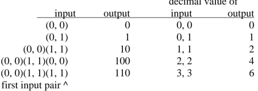
8 •• Binary adder This is a transducer with binary inputs occurring in pairs. That is,
the input alphabet is all pairs over {0, 1}: {(0, 0), (0, 1), (1, 0), (1, 1)}. The inputs are to be interpreted as bits of two binary numerals, least-significant bit first as in the previous problem. The output is a numeral representing the sum of the inputs, also least-significant bit first. As before, we need to input a final (0, 0) if we wish to see the final answer.
decimal value of input output input output
(0, 0) 0 0, 0 0
(0, 1) 1 0, 1 1
(0, 0)(1, 1) 10 1, 1 2
(0, 0)(1, 1)(0, 0) 100 2, 2 4
(0, 0)(1, 1)(1, 1) 110 3, 3 6
first input pair ^
Answer: Apparently only the value of the "carry" needs to be remembered from
one state to the next. Since only two values of carry are possible, this tells us that two states will be adequate.
c1 c0
(0, 0) / 0 (0, 1) / 1 (1, 0) / 1
(1, 1) / 0 (0, 0) / 1
(0, 1) / 0 (1, 0) / 0 (1, 1) / 1
Figure 212: Serial binary adder, least-significant bits first
9 ••• MB3 (multiply-by-three) Similar to MB2, except the input is multiplied by 3.
For example
decimal value of input output input output
0 0 0 0
01 11 1 3
010 110 2 6
001011 100001 11 33
Note that two final 0's might be necessary to get the full output. Why?
10 •••• MBN (multiply-by-n, where n is a fixed natural number) (This is a separate
problem for each n.) This machine is a transducer with binary input and outputs, both least-significant bit first, producing a numeral that is n times the input.
11 ••• Binary maximum This is similar to the adder, but the inputs occur most-significant digit first and both inputs are assumed to be the same length
numeral.
decimal value of
input output input output
(0, 0) 0 0, 0 0
(0, 1) 1 0, 1 1
(0, 1)(1, 1) 11 1, 3 3
(0, 1)(1, 1)(1, 0)110 3, 6 6
(1, 1)(1, 0)(0, 1)110 6, 5 6
^ first input pair
12 •• Maximum classifier This is a classifier version of the preceding. There are
three possible outputs assigned to a state: {tie, 1, 2}, where 1 indicates that the first input sequence is greater, 2 indicates the second is greater, and 'tie' indicates that the two inputs are equal so far.
input class
(1, 1) tie
(1, 1)(0, 1) 2
(1, 1)(0, 1)(1, 1) 2 (1, 0)(0, 1)(1, 1) 1
13 •• 1DB3 (Unary divisible by 3) This is an acceptor with input alphabet {1}. It
accepts exactly those strings having a multiple of three 1's (including
λ
).14 ••• 2DB3 (Binary divisible by 3) This is an acceptor with input alphabet {0, 1}. It
accepts exactly those strings that are a numeral representing a multiple of 3 in binary, least-significant digit first. (Hint: Simulate the division algorithm.) Thus the accepted strings include: 0, 11, 110, 1001, 1100, 1111, 10010, ... 15 ••• Sequential combination locks (an infinite family of problems): A single
string over the alphabet is called the "combination". Any string containing this combination is accepted by the automaton ("opens the lock"). For example, for the combination 01101, the acceptor is:
0
0
a 1
0 1
0
0, 1
b c d e f
0
1 1
1
Figure 213: A combination lock state diagram
The tricky thing about such problems is the construction of the backward arcs; they do not necessarily go back to the initial state if a "wrong" digit is entered, but only back to the state that results from the longest usable suffix of the digits entered so far. The construction can be achieved by the "subset" principle, or by devising an algorithm that will produce the state diagram for any given combination lock problem. This is what is done in a string matching algorithm known as the "Knuth-Morris-Pratt" algorithm.
Construct the state-diagram for the locks with the following different combinations: 1011; 111010; 010010001.
16 ••• Assume three different people have different combinations to the same lock. Each combination enters the user into a different security class. Construct a classifier for the three combinations in the previous problem.
17 ••• The preceding lock problems assume that the lock stays open once the combination has been entered. Rework the example and the problems assuming that the lock shuts itself if more digits are entered after the correct combination, until the combination is again entered.
12.2 Finite-State Grammars and Non-Deterministic Machines
An alternate way to define the language accepted by a finite-state acceptor is through a grammar. In this case, the grammar can be restricted to have a particular form of production. Each production is either of the form:
N
→ σ
Mwhere N and M are auxiliaries and
σ
is a terminal symbol, or of the form N→ λ
recalling that
λ
is the empty string. The idea is that auxiliary symbols are identifiedwith states. The start state is the start symbol. For each transition in an acceptor for the
language, of the form
Figure 214: State transition corresponding to a grammar production
there is a corresponding production of the form q1
→ σ
q2In addition, if q2 happens to be an accepting state, there is also a production of the form. q2
→ λ
Example: Grammar from Acceptor
For our acceptor for exactly one edge, we can apply these two rules to get the following grammar for generating all strings with one edge:
The start state is a. The auxiliaries are {a, b, c, d, e, f}. The terminals are {0, 1}. The productions are:
a
→
0b c→
0ea
→
1c c→
1cb
→
0b e→
0eb
→
1d e→
1fd
→
0f e→ λ
d
→
1d f→
0fd
→ λ
f→
1fTo see how the grammar derives the 1-edged string 0011 for example, the derivation tree is:
a
0 b
0 b
1 d
1 d
λ
Figure 215: Derivation tree in the previous finite-state grammar, deriving the 1-edged string 0011
While it is easy to see how a finite-state grammar is derived from any finite-state acceptor, the converse is not as obvious. Difficulties arise in productions that have the same lefthand-side with the same terminal symbol being produced on the right, e.g. in a grammar, nothing stops us from using the two productions
a
→
0b a→
0cYet this would introduce an anomaly in the state-transition diagram, since when given input symbol 0 in state a, the machine would not know to which state to go next:
b
c 0
a 0
Figure 216: A non-deterministic transition
This automaton would be regarded as non-deterministic, since the next state given input 0 is not determined. Fortunately, there is a way around this problem. In order to show it, we first have to define the notion of "acceptance" by a non-deterministic acceptor.
A non-deterministic acceptor accepts a string if there is some path from a starting state to an accepting state having a sequence of arc labels equal to that string.
We say a starting state, rather than the starting state, since a non-deterministic acceptor is allowed to have multiple starting states. It is useful to also include λ transitions in non-deterministic acceptors. These are arcs that have λ as their label. Since λ designates the empty string, these arcs can be used in a path but do not contributed any symbols to the sequence.
Example: Non-deterministic to Deterministic Conversion
Recall that a string in the language generated by a grammar consists only of terminal symbols. Suppose the productions of a grammar are (with start symbol a, and terminal alphabet {0, 1}):
a
→
0d b→
1ca
→
0b b→
1a
→
1 d→
0dc
→
0b d→
1The language defined by this grammar is the set of all strings ending in 1 that either have exactly one 1 or that consist of alternating 01. The corresponding (non-deterministic) automaton is:
0 d b 0 a 0 1 1 1 c 0 1 e
Figure 217: A non-deterministic automaton that accepts the set of all strings ending in 1that have exactly one 1 or consist of an alternating 01's.
There are two instances of non-determinism identifiable in this diagram: the two 0-transitions leaving a and the two 1-0-transitions leaving b. Nonetheless, we can derive from this diagram a corresponding deterministic finite-automaton. The derivation results in the deterministic automaton shown below.
0 0 A 1 0 B 1 D C E 1 1
0, 1 O
0, 1 0 0 0 0 1 F
Figure 218: A deterministic automaton that accepts the set of all strings ending in 1 that have exactly one 1 or consist of an alternating 01's.
We can derive a deterministic automaton D from the non-deterministic one N by using
subsets of the states of N as states of D. In this particular example, the subset associations
are as follows: A ~ {a} B ~ {b, d} C ~ {c, e} D ~ {d} E ~ {e} F ~ {b} O ~ {}
General method for deriving a deterministic acceptor D from a non-deterministic one N:
The state set of D is the set of all subsets of N.
The initial state of D is the set of all initial states of N, together with states reachable from initial states in N using only λ transitions.
There is a transition from a set S to a set T of D with label
σ
(whereσ
is a single input symbol).T = {q' | there is a q in S with a sequence of transitions from q to q' corresponding to a one symbol string
σ
}The reason we say sequence is due to the possibility of λ transitions; these do not add any new symbols to the string. Note that λ is not regarded as an input symbol.
The accepting states of the derived acceptor are those that contain at least one accepting state of the original acceptor.
In essence, what this method does is "compile" a breadth-first search of the non-deterministic state graph into a non-deterministic finite-state system. The reason this works is that the set of all subsets of a finite set is finite.
Exercises
Construct deterministic acceptors corresponding to the following non-deterministic acceptors, where the alphabet is {0, 1}.
1 •
a 0 b
2 •
a 0 b
1
3 ••
a 0
1
0 1
4 ••
a 1 b 0 c
0 1
12.3 Meaning of Regular Expressions
From the chapter on grammars, you already have a good idea of what regular expressions mean already. While a grammar for regular expression was given in that chapter, for purposes of giving a meaning to regular expressions, it is more convenient to use a grammar that is intentionally ambiguous, expressing constructs in pairs rather than in sequences:
R
→
'λ
' R→ ∅
R
→ σ
, for each letterσ
in AR
→
R R // juxtapositionR
→
( R | R ) // alternationR
→ (
R)* // iterationTo resolve the ambiguity in the grammar, we simply "overlay" on the grammar some conventions about precedence. The standard precedence rules are:
* binds more tightly than either juxtaposition or | juxtaposition binds more tightly than |
We now wish to use this ambiguous grammar to assign a meaning to regular expressions. With each expression E, the meaning of E is a language, i.e. set of strings, over the alphabet A. We define this meaning recursively, according to the structure of the grammar:
Basis:
• L(
λ
) is {λ
}, the set consisting of one string, the empty stringλ
. • L(∅
) is∅
, the empty set.• For each letter
σ
in A, and L(σ
) is {σ
}, the set consisting of one string of one letter,σ
.Induction rules:
• L(RS) = L(R)L(S), where by the latter we mean the set of all strings of the form of the concatenation rs, where r
∈
L(R) and s∈
L(S).• L(R | S) = L(R)
∪
L(S). • L(R*) = L(R)*To clarify the first bullet, for any two languages L and M, the "set concatenation" LM is defined to be {rs | r
∈
L and s∈
M}. That is, the "concatenation” of two sets of strings is the set of all possible concatenations, one string taken from the first set and another taken from the second. For example,{0}{1} is defined to be {01}.
{0, 01}{1, 10} is defined to be {01, 010, 011, 0110}.
{01}{0, 00, 000, ...} is defined to be {010, 0100, 01000, ...}.
To explain the third bullet, we need to define the * operator on an arbitrary language. If L is a language, the L* is defined to be (using the definition of concatenation above)
{
λ
}∪
L∪
LL∪
LLL∪
...That is, L* consists of all strings formed by concatenating zero or more strings, each of which is in L.
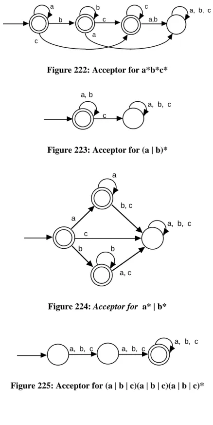
Regular Expression Examples over alphabet {a, b, c}
Expression Set denoted
a | b | c The set of 1-symbol strings {"a", "b", "c"}
λ
| (a | b | c) | (a | b | c)(a | b | c) The set of strings with two or fewer symbolsa* The set of strings using only symbol a
a*b*c* The set of strings in which no a follows a b
and no a or b follows a c
(a | b)* The set of strings using only a and b.
a* | b* The set of strings using only a or only b
(a | b | c)(a | b | c)(a | b | c)* The set of strings with at least two symbols.
((b | c)* ab (b | c)*)* The set of strings in which each a is immediately followed by a b.
(b | c)* | ((b | c)* a (b | c) (b | c)*)* (
λ
| a) The set of strings with no two consecutiveRegular expressions are finite symbol strings, but the sets they denote can be finite or infinite. Infinite sets arise only by virtue of the * operator (also sometimes called the Kleene-star operator).
Identities for Regular Expressions
One good way of becoming more familiar with regular expressions is to consider some identities, that is equalities between the sets described by the expressions. Here are some examples. The reader is invited to discover more.
For any regular expressions R and S: R | S = S | R
R |
∅
= R∅
| R = RR
λ
= Rλ
R = RR
∅
=∅
∅
R =∅
λ
*=λ
∅
* =λ
R*=λ
| RR* (R |λ
)*= R* (R*)* = R*Exercises
1 •• Determine whether or not the following are valid regular expression identities:
λ∅
=λ
R (S | T) = RS | RT R*=
λ
| R*R RS = SR(R| S)* = R* | S* R*R = RR*
(R* | S*)* = (R| S)* (R*S*) = (R | S)*
For any n, R*=
λ
| R| RR | RRR| .... | Rn-1 | RnR*, where Rn is an abbreviation for RR....R.n times
2 ••• Equations involving languages with a language as an unknown can sometimes be solved using regular operators. For example,
S = RS | T
3 ••• Suppose that we have grammars that respectively generate sets L and M as languages. Show how to use these grammars to form a grammar that generates each of the following languages
L
∪
MLM L*Regular Languages
The regular operators (|, *, and concatenation) are applicable to any languages. However, a special name is given to languages that can be constructed using only these operators and languages consisting of a single string, and the empty set.
Definition: A language (set of strings over a given alphabet) is called regular if it is a
set of strings denoted by some regular expression. (A regular language is also called a
regular set.)
Let us informally explore the relation between regular languages and finite-state acceptors. The general idea is that the regular languages exactly characterize sets of paths from the initial state to some accepting state. We illustrate this by giving an acceptor for each of the above examples.
a, b, c a, b, c
a, b, c
Figure 219: Acceptor for a | b | c
a, b, c a, b, c a, b, c a, b, c
Figure 220: Acceptor for
λ
| (a | b | c) | (a | b | c)(a | b | c) a, b, ca
b, c
a,b
b a, b, c
a b
c
c
c
a
Figure 222: Acceptor for a*b*c*
a,
a, b, c c
b
Figure 223: Acceptor for (a | b)*
a
a, b, c c
b
a
b b, c
a, c
Figure 224: Acceptor for a* | b*
a, b, c a, b, c
a, b, c
b,c
a a,c
a, b, c
b a
b,c
Figure 226: Acceptor for ((b | c)* ab (b | c))*
As we can see, the connection between regular expressions and finite-state acceptors is rather close and natural. The following result makes precise the nature of this relationship.
Kleene's Theorem (Kleene, 1956) A language is regular iff it is accepted
by some finite-state acceptor.
The "if" part of Kleene's theorem can be shown by an algorithm similar to Floyd's algorithm. The "only if" part uses the non-deterministic to deterministic transformation.
The Language Accepted by a Finite-State Acceptor is Regular
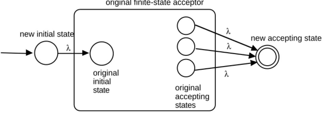
The proof relies on the following constructive method:
Augment the graph of the acceptor with a single distinguished starting node and accepting node, connected via
λ
-transitions to the original initial state and accepting states in the manner shown below. The reason for this step is to isolate the properties of being initial and accepting so that we can more easily apply the transformations in the second step.original initial state
original finite-state acceptor
new accepting state new initial state
original accepting states
λ
λ λ λ
One at a time, eliminate the nodes in the original acceptor, preserving the set of paths through each node by recording an appropriate regular expression between each pair of other nodes. When this process is complete, the regular expression connecting the initial state to the accepting state is the regular expression for the language accepted by the original finite-state machine.
To make the proof complete, we have to describe the node elimination step. Suppose that prior to the elimination, the situation is as shown below.
X Z
y xz
R R
xy yz
yy R R
Figure 228: A situation in the graph before elimination of node y
Here x and z represent arbitrary nodes and y represents the node being eliminated. A variable of the form Rij represents the regular expression for paths from i to j using nodes previously eliminated. Since we are eliminating y, we replace the previous expression Rxz with a new expression
Rxz | Rxy Ryy* Ryz
The rationale here is that Rxz represents the paths that were there before, and Rxy Ryy* Ryz represents the paths that went through the eliminated node y.
X xz Z
R
| Rxy Ryy Ryz*
Figure 229: The replacement situation after eliminating node y
The catch here is that we must perform this updating for every pair of nodes x, z, including the case where x and z are the same. In other words, if there are m nodes left, then m2 regular expression updates must be done. Eliminating each of n nodes then requires O(n3) steps. The entire elimination process is very similar to the Floyd and Warshall algorithms discussed in the chapter on Complexity. The only difference is that here we are dealing with the domain of regular expressions, whereas those algorithms dealt with the domains of non-negative real numbers and bits respectively.
Prior to the start of the process, we can perform the following simplification:
Any states from which no accepting state is reachable can be eliminated, along with arcs connecting to or from them.
Example: Regular Expression Derivation
Derive a regular expression for the following finite-state acceptor:
1 b 2
b
a
3 b
4 a
a, b a
Figure 230: A finite-state acceptor from which a regular expression is to be derived
First we simplify by removing node 4, from which no accepting state is reachable. Then we augment the graph with two new nodes, 0 and 5, connected by
λ
-transitions. Notice that for some pairs of nodes there is no connection. This is equivalent to the corresponding regular expression being∅
. Whenever∅
is juxtaposed with another regular expression, the result is equivalent to∅.
Similarly, wheneverλ
is juxtaposed with another regular expression R, the result is equivalent to R itself.0
a
1 b 2 5
λ
a
b b
3
λ
λ
Figure 231: The first step in deriving a regular expression. Nodes 0 and 5 are added.
Now eliminate one of the nodes 1 through 3, say node 1. Here we will use the identity that states
λ
a*b = a*b.0
aa*b
2 5
3 b b
a * b λ
λ
Figure 232: After removal of node 1
Next eliminate node 2.
0 5
3
b b aa b
* *
a ( * )
λ
b aa b a∗ ( ∗ ) b∗
Figure 233: After removal of node 2
Finally eliminate node 3.
0 a *b )
* aa
( b | a * b (aa b) b b* * *
5 *
Figure 234: After removal of node 1
The derived regular expression is
Every Regular Language is Accepted by a Finite-State Acceptor
We already know that we can construct a deterministic finite-state acceptor equivalent to any deterministic one. Hence it is adequate to show how to derive a non-deterministic finite-state acceptor from a regular expression. The paths from initial node to accepting node in the acceptor will correspond in an obvious way to the strings represented by the regular expression.
Since regular expressions are defined inductively, it is very natural that this proof proceed along the same lines as the definition. We expect a basis, corresponding to the base cases
λ
,∅
, andσ
(forσ
each in A). We then assume that an acceptor is constructable for regular expressions R and S and demonstrate an acceptor for the cases RS, R | S, and R*. The only thing slightly tricky is connecting the acceptors in the inductive cases. It might be necessary to introduce additional states in order to properly isolate the paths in the constituent acceptors. Toward this end, we stipulate that(i) the acceptors constructed shall always have a single initial state and single accepting state.
(ii) no arc is directed from some state into the initial state Call these property P.
Basis: The acceptors for
λ
,∅
, andσ
(forσ
each in A) are as shown below:Figure 235: Acceptor for
∅
with property Pλ
Figure 236: Acceptor for
λ
(the empty sequence) with property Pσ
Induction Step: Assume that acceptors for R and S, with property P above, have been
constructed, with their single initial and accepting states as indicated on the left and right, respectively.
R S
Figure 238: Acceptors assumed to exist for R and S respectively, having property P
Then for each of the cases above, we construct new acceptors that accept the same language and which have property P, as now shown:
R S
λ
formerly accepting, now non-accepting
Figure 239: Acceptor for RS, having property P
R
S
λ λ
λ λ
R
λ
λ λ
λ
Figure 241: Acceptor for R*, having property P
Regular expressions in UNIX
Program egrep is one of several UNIX tools that use some form of regular expression for pattern matching. Other such tools are ed, ex, sed, awk, and archie. The notations appropriate for each tool may differ slightly. Possible usage:
egrep regular-expression filename
searches the file line-by-line for lines containing strings matching the regular-expression and prints out those lines. The scan starts anew with each line. In the following description, 'character' means excluding the newline character:
A single character not otherwise endowed with special meaning matches that character. For example, 'x' matches the character x.
The character '.' matches any character.
A regular expression followed by an * (asterisk) matches a sequence of 0 or more matches of the regular expression.
Effectively a regular expression used for searching is preceded and followed by an implied .*, meaning that any sequence of characters before or after the string of interest can exist on the line. To exclude such sequences, use ^ and $:
The character ^ matches the beginning of a line.
The character $ matches the end of a line.
A regular expression followed by a + (plus) matches a sequence of 1 or more matches of the regular expression.
A regular expression followed by a ? (question mark) matches a sequence of 0 or 1 matches of the regular expression.
A \ followed by a single character other than newline matches that character. This is used to escape from the special meaning given to some characters.
A string enclosed in brackets [] matches any single character from the string. Ranges of ASCII character codes may be abbreviated as in a-z0-9, which means all characters in the range a-z and 0-9. A literal - in such a context must be placed after \ so that it can't be mistaken as a range indicator.
Two regular expressions concatenated match a match of the first followed by a match of the second.
Two regular expressions separated by | or newline match either a match for the first or a match for the second.
A regular expression enclosed in parentheses matches a match for the regular expression.
The order of precedence of operators at the same parenthesis level is [] then *+? then concatenation then | and newline.
Care should be taken when using the characters $ * [ ] ^ | ( ) and \ in the expression as they are also meaningful to the various shells. It is safest to enclose the entire
expression argument in single quotes.
Examples: UNIX Regular Expressions
Description of lines to be selected Regular Expression
containing the letters qu in combination qu
beginning with qu ^qu
ending with az az$
beginning with qu and ending with az ^qu.*az$
containing the letters qu or uq uq|qu
containing two or more a's in a row a.*a
containing four or more i's i.*i.*i.*i
containing five or more a's and i's [ai].*[ai].*[ai].*[ai].*[ai]
containing ai at least twice (ai).*(ai)
containing uq or qu at least twice (uq|qu).*(uq|qu) Exercises
Construct deterministic finite-state acceptors for the following regular expressions: 1 • 0*1*
3 •• (01 | 011)* 4 •• (0* | (01)*)*
5 •• (0 | 1)*(10110)(0 | 1)*
6 ••• The regular operators are concatenation, union ( | ), and the * operator. Because any combination of regular languages using these operators is itself a regular language, we say that the regular languages are closed under the regular operators. Although intersection and complementation (relative to the set of all strings,
Σ
*) are not included among the regular languages, it turns out that the regular languages are closed under these operators as well. Show that this is true, by using the connection between regular languages and finite-state acceptors. 7 ••• Devise a method for determining whether or not two regular expressions denotethe same language.
8 •••• Construct a program that inputs a regular expression and outputs a program that accepts the language denoted by that regular expression.
9 ••• Give a UNIX regular expression for lines containing floating-point numerals.
12.4 Synthesizing Finite-State Machines from Logical Elements
We now wish to extend techniques for the implementation of functions on finite domains in terms of logical elements to implementing finite-state machines. One reason that this is important is that digital computers are constructed out of collections of finite-state machines interconnected together.As already stated, the input sequences for finite-state machines are elements of an infinite set
Σ
*, whereΣ
is the input alphabet. Because the output of the propositional functions we studied earlier were simply a combination of the input values, those functions are called combinational, to distinguish them from the more general functions onΣ
*, which are called sequential.We will show how the implementation of machines can be decomposed into combinational functions and memory elements, as suggested by the equation
Sequential Function = Combinational Functions + Memory
Recall the earlier structural diagrams for transducer and classifiers, shown as "feedback" systems. Note that these two diagrams share a common essence, namely the next-state portion. Initially, we will focus on how just this portion is implemented. The rest of the machine is relatively simple to add.
F
∆
next-state function
delay or memory
input
Figure 242: The essence of finite-state machine structure
Implementation using Logic Elements
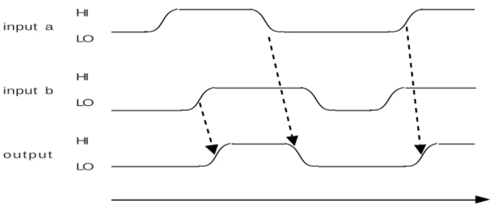
Before we can "implement" such a diagram, we must be clearer on what items correspond to changes of input, output, and state. The combinational logical elements, such as AND-gates and OR-AND-gates, as discussed earlier are abstractions of physical devices. In those devices, the logical values of 0 and 1 are interpretations of physical states. The output of a device is a function of its inputs, with some qualification. No device can change state instantaneously. When the input values are first presented, the device's output might be in a different state from that indicated by the function. There is some delay time or
switching time associated with the device that must elapse before the output stabilizes to
the value prescribed by the function. Thus, each device has an inherent sequential behavior, even if we choose to think of it as a combinational device.
Example Consider a 2-input AND-gate. Suppose that a device implements this gate due
to our being able to give logical values to two voltages, say LO and HI, which correspond to 0 and 1 respectively. Then, observed over time, we might see the following behavior of the gate in response to changing inputs. The arrows in the diagram indicate a causal relationship between the input changes and output changes. Note that there is always some delay associated with these changes.
HI LO
HI LO
HI LO input a
input b
o u t p u t
t i m e
Modeling the sequential behavior of a device can be complex. Computer designers deal with an abstraction of the behavior in which the outputs can only change at specific instants. This simplifies reasoning about behaviors. The abstract view of the AND-gate shown above can be obtained by straightening all of the changes of the inputs and outputs, to make it appear as if they were instantaneous.
HI LO HI LO HI LO input a
input b
o u t p u t
t i m e
Figure 244: An abstraction of the sequential behavior of an AND-gate
Quantization and Clocks
In order to implement a sequential machine with logic gates, it is necessary to select a scheme for quantizing the values of the signal. As suggested by the preceding diagram, the signal can change continuously. On the other hand, the finite-state machine abstraction requires a series of discrete input and output values. For example, as we look at input a in the preceding diagram, do we say that the corresponding sequence is 0101 based on just the input changes? If that were the case, what would be the input corresponding to sequence 00110011? In other words, how do we know that a value that stays high for some time is a single 1 or a series of 1's? The most common means of resolving this issue is to use a system-wide clock as a timing standard. The clock "ticks" at regular intervals, and the value of a signal can be sampled when this tick occurs.
The effect of using a clock is to superimpose a series of tick marks atop the signals and agree that the discrete valued signals correspond to the values at the tick marks. Obviously this means that the discrete interpretation of the signals depends on the clock interval. For example, one quantization of the above signals is shown as follows:
HI LO
HI LO
HI LO input a
input b
o u t p u t
t i m e
01001
01101
01101
Figure 245: AND-gate behavior with one possible clock quantization
Corresponding to the five ticks, the first input sequence would be 01001, the second would be 01101, and the output sequence would be 01101. Notice that the output is not quite the AND function of the two inputs, as we might have expected. This is due to the fact that the second output change was about to take place when the clock ticked and the previous output value carried over. Generally we avoid this kind of phenomenon by designing such that the changes take place between ticks and at each tick the signals are, for the moment, stable.
The next figure shows the same signals with a slightly wider clock interval superimposed. In this instance, no changes straddle the clock ticks, and the input output sequences appear to be what is predicted by the definition of the AND function.
HI LO
HI LO
HI LO input a
input b
o u t p u t
t i m e
0101
0101
0101
Figure 246: AND-gate behavior with wider quantization
Flip-Flops and Clocks
As stated above, in order to maintain the effect of instantaneous changes when there really is no such thing, the inputs of gates are only sampled at specific instants. By using the value of the sample, rather than the true signal, we can approach the effect desired. In order to hold the value of the sample from one instant to the next, a memory device known as a D flip-flop is used.
The D flip-flop has two different kinds of inputs: a signal input and a clock input. Whenever the clock "ticks", as represented, say, by the rising edge of a square wave, the signal input is sampled and held until the next tick. In other words, the flip-flop "remembers" the input value until the next tick; then it takes on the value at that time.